Fine Spatial Information Represented in a Population of Retinal Ganglion Cells

Abstract

Detailed measurement of ganglion cell receptive fields often reveals significant deviations from a smooth, Gaussian profile. We studied the effect of these irregularities on the representation of fine spatial information in the retina. We recorded from nearby clusters of ganglion cells, testing their ability to determine the location of small flashed spots, and we compared the results to the prediction of a Gaussian receptive field model derived from reverse correlation. Despite considerable receptive field overlap, almost all ganglion cell pairs signaled nearly independently. For groups of five cells with highly overlapping receptive fields, the measured light-evoked currents encoded ∼33% more information than predicted by the Gaussian receptive field model. Including measured local irregularities in the receptive field model increased performance to the level observed experimentally. These results suggest that instead of being an unavoidable defect, irregularities may be a positive design feature of population neural codes.

Introduction

In the retina, visual information originating in photoreceptors is propagated via a network of bipolar and amacrine cells to retinal ganglion cells. Models of early visual processing assume that visual space is sampled by a regular array of smooth, approximately Gaussian receptive fields (Rodieck, 1965; Atick and Redlick, 1990; Borghuis et al., 2008; Pillow et al., 2008). This approximation is attractive because it is analytically tractable and is consistent with receptive fields measured by spatial gratings and coarse (50–100 μm) checkerboards. One problem with these models, however, is that spatial gratings and coarse checkerboards average over fine spatial inhomogeneities, smoothing the measured receptive field. Measurements with fine checkerboards and fine spatial gratings show that receptive fields of individual cells not only vary in size, position and orientation, but often contain localized regions of high or low sensitivity (Brown et al., 2000; Passaglia et al., 2002; Gauthier et al., 2009; Field et al., 2010), which we refer to as “local irregularities.”

Previous studies have focused primarily on how variability in receptive field size, position and orientation affect visual encoding in mosaics of single types of ganglion cells (Wässle and Boycott, 1991), in which receptive fields tile the retina in a regular array with little overlap. Variability in receptive field size, position and orientation has been proposed to degrade performance by causing regions to be nonuniformly sampled (Brown et al., 2000) or improve performance by allowing ganglion cells to sample regions more uniformly despite variability in the retinal mosaic lattice (Gauthier et al., 2009; Liu et al., 2009).

It is possible, however, that local irregularities within receptive fields strongly affect the concerted signaling of the entire population of ganglion cells. Each retinal location is sampled by many ganglion cells from multiple mosaics, with the entire population having highly overlapping receptive fields (Devries and Baylor, 1997; Dacey et al., 2003; Segev et al., 2004), and multiple cell types converge onto the same major projection centers in the brain (Dacey et al., 2003; Berson, 2008). Local irregularities will tend to decorrelate the responses of neighboring ganglion cells with overlapping receptive fields, potentially resulting in a large increase in the total information conveyed by the population.

We ask here how local irregularities in overlapping receptive fields contribute to the information in the inputs to groups of cells within a small patch of retina. While the output encoding of the visual signal involves the additional nonlinear transformation of spike generation, we examined input currents so that we could measure information free from assumptions about the nature of the population spike code and the sampling issues associated with measuring distributions of population spiking activity.

We find that, despite taking into account the size and placement of ganglion cell receptive fields as well as their noise, the inner retina encodes significantly more information about a fine spatial stimulus than expected from a Gaussian receptive field model. The model's failure is corrected after local receptive field irregularities are taken into account. These results suggest that, for highly overlapping receptive fields, local irregularities are not an unwanted imperfection, but instead contribute significantly to the retina's ability to encode spatial detail.

Materials and Methods

Preparation of the retina.

Experiments were performed on larval tiger salamanders (Ambystoma tigrinum, Charles D. Sullivan Co. Ltd.). After 3–10 h in darkness, the animal was rapidly decapitated and the head and spinal cord were pithed. The eyes were removed and hemisected under infrared illumination, using infrared/visible converters. The posterior half of each eye was transferred to a Petri dish filled with chilled (4°C) bicarbonate buffered Ringer's solution (concentrations in mm): 110 NaCl, 2 KCl, 1.6 MgCl, 30 NaHCO₃, 0.01 EDTA, 1.5 CaCl₂, osmolarity 260, and pH 7.4 when equilibrated with 95%O₂, 5% CO₂, 20–22°C. After a brief period of incubation (10–30 min) to allow the retina to separate from the pigment epithelium, the retina was cut radially into thirds and placed, photoreceptor side down, on the recording chamber. The glass of the chamber had been made sticky by washing in 5% HCl 95% EtOH, incubating with 1% concavalin A for 10–30 min (Sigma) and rinsed in distilled water. The preparation was placed onto the microscope under infrared illumination, and continuously perfused with bicarbonate buffered solution. In some cases, the second eyecup was kept at 4°C and used several hours later.

To gain access to the retinal ganglion cell layer, the inner limiting membrane (ILM) was gently torn using a pair of glass pipettes mounted in opposing micromanipulators, exposing 4–10 cells (Kim and Rieke, 2001). Once a hole was torn, the microscope was focused down onto the photoreceptor layer and the retina moved laterally, out of the field of view. The stimulus projection system was then focused and calibrated with custom written calibration software. The retina was moved back into place, and 20–30 cone photoreceptors were chosen by their appearance (smaller than the rod photoreceptors) and location (regularly nestled between 4 and 5 surrounding rod photoreceptors, in semiregular lattice). An example is shown in Figure 1.

Figure 1.

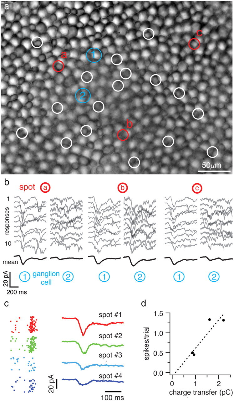
The responses of retinal ganglion cells to small flashed spots. a, The photoreceptor mosaic imaged under infrared illumination. The location and size of 20 spot stimuli are shown by white circles; three spots are highlighted in red (a–c). The blurring in the central area of the image is due to tearing of the inner limiting membrane to gain access to the ganglion cells, but is not expected to affect the focus or intensity of the spots, which are projected from the photoreceptor side of the retina. Soma locations of the ganglion cells being recorded are indicated by the blue circles. b, Responses of the two simultaneously recorded ganglion cells to three flashed spots. Each gray trace is the excitatory current response of a ganglion cell to one presentation of a spot flashed at the beginning of the trial. Ten of 60 trials for each spot are shown. The average response across a block of trials is shown in black. c, Spike rasters (60 repeated trials) and input currents from a different ganglion cell responding to spots in four different locations (rows). d, Integrated charge transfer versus spike count for the data in c. Both measures use a time window of 200 ms starting from flash onset.

Electrophysiology.

Whole-cell patch pipette electrodes (1 μm tip diameter, 7–12 MΩ) were made by pulling ω-dot glass (FHC Inc.) on a pipette puller (MP-2000, Sutter Instruments). Electrodes were filled with an internal physiological salt solution (in mm): 115 Cs-aspartate, 20 CsCl, 10 HEPES, 1 N-methylglucamine (NMG) EGTA, and 0.2 CaCl₂; pH was adjusted to 7.2 with NMG-OH, and osmolarity was 260–265 mOsm (Kim and Rieke, 2003). A pair of electrodes were mounted on the patch amplifier headstages (Axon Axopatch 700B) and advanced to the ganglion cell surface using remote-controlled micromanipulators (Sutter) while being viewed under infrared illumination (Kodak Wratten 700B). Typical total series resistance was 100–500 MΩ, and cells were maintained at a holding potential of −70 mV unless noted. The junction potential was not corrected. A typical recording from a ganglion cell lasted 30 min to 1 h. Current-clamp recordings were made from cells with input resistances of <100 MΩ, membrane capacitances on the order of 20–40 pF and action potentials with peak voltages exceeding 0 mV. Spike times were extracted from threshold crossings.

Visual stimulus.

The photoreceptor mosaic was visualized under infrared illumination and 20 locations within a typical ganglion cell's receptive field center (radius ∼300 μm) were chosen (Fig. 1a). The location of spots was chosen to coincide with the cone photoreceptors, which are nestled in a semiregular array among the larger rod photoreceptors. A pair of cells in the ganglion cell layer was recorded in whole-cell configuration (Fig. 1b). At each stimulus location, a spot was flashed, one at a time, in random sequence, with a 1 s delay between flashes. The spots were red (670 nm) to preferentially stimulate L-cones and were sufficiently short and intense (50 ms, 3000 photons/cone/s) to provoke a brief impulse response. The retina was continuously illuminated by a rod-suppressing 540 nm green background.

Stimuli were delivered using a digital mirror device (DMD) (Discovery 3000, Texas Instruments) projected through a 10× apochromatic objective (Nikon) mounted in place of the condenser of the microscope (Nikon FN-1). A circular mask of 300 μm in diameter restricted the image to a central area. A high-power RGB LED (SuperBrightLEDS) behind a holographic diffuser (ThorLabs) was focused upon the DMD through a total internal reflection prism, which folds the light path and allows only “on” state light to be reflected into the rest of the optical system. The image of the light-emitting diode (LED) was focused on the entrance pupil of the relay lens. This Kohler-type illumination produced a bright and uniform field (∼10–20% variation, data not shown) and high contrast ratio (10000:1), with a minimum of chromatic aberration (3–5 μm in the z-axis between red and blue images) and a point spread function 2–3 μm wide at half-maximum. Power measurements were taken with a calibrated power meter at the specimen plane (Newport) and used to calculate the control signal to apply to the LED to generate the desired photon flux. Salamander photoreceptor spectra were taken from values reported in the literature (Makino et al., 1991; Ma et al., 2001). The continuous background light was generated by a green LED, whose diffused image was projected onto the retina from the ganglion-cell side through the microscope objective.

The DMD was controlled through a digital visual interface (FakeSpace Labs) in which the 24 bit planes of an RGB image were sequentially shown on the DMD, resulting in a binary frame rate of 24 × 60 Hz = 1440 Hz. The DMD interface and the data acquisition signals were synchronized using a custom timing board that generated TTL signals for the 60 and 1440 Hz frames as well as a bit-code for the upper-left hand pixel of the current frame. This code was used to mark the start of a trial, the presentation of the spots, and a unique number assigned to the trial. The stimulus software was written in Visual C++ and OpenGL.

Data analysis.

Currents were low-pass filtered at 4 kHz, digitized at 10 kHz, and recorded to disk using custom software written in LabView (National Instruments). Subsequent analysis was done in Mathematica (Wolfram Research). Each experiment consisted of several hundred or thousand trials in pseudo-random order. Trials in the data record were identified and annotated in a database.

To calculate the principal components of the responses in a single ganglion cell, all of the trials (excluding trials in which no spot was presented, and the first and last trials) were mean subtracted and placed in a two dimensional matrix, where each row is a single trial. The principal components of variance were calculated using the PrincipalComponents routine in Mathematica and the first three principal components were extracted (Fig. 2a). The response amplitude for a given trial was then calculated by taking the dot product between the response to that trial and the first principal component. In general, the second or third principal component may also carry information about the identity of the flashed spot. There appeared, however, to be little additional information in the second or third principal components for a given cell: the same plots generated using the second or third components (rather than the first) appeared to be randomly scattered. This was confirmed with calculation of the mutual information using the second and third principal components.

Figure 2.

Most of the signal variance is captured by the first principal component of the response. a, First three principal components (black, red, and blue are first, second, and third, respectively) of the responses of the two ganglion cells shown in Figure 1a,b. Principal components are shown with baseline subtracted for clarity. b, Distribution of signal and noise power among the first 10 principal components. Red trace is mean squared power of the ith principal component across all trials, while blue trace is mean squared power of the ith principal component across non-flash trials only. The inset shows the same data on an enlarged scale. Error bars are SEM. The table shows the fraction of the signal power (power in all trials − power in non-flash trials) in the first 10 components.

In many recordings, the response amplitudes in a ganglion cell slowly increased or decreased over the course of the experiment. This drift was corrected by calculating a multiplicative scale factor. Because the trials were randomized, the scale factor was calculated by taking the average response in a moving window of 20 trials (so that responses to all spots were included) and normalizing the responses by the scale factor. This drift correction did not change the results presented here.

To calculate the percentage of the signal variance accounted by the ith principal component, the fraction of the total signal power (power from all trials − power from trials where no flash was presented) from each component was calculated:

where N is the total number of PCA components, and

and i is the ith PCA component.

Calculation of mutual information.

By definition, the mutual information between stimulus s and response r for our stimulus is:

where K is the number of spots (in this case presented with equal frequency), r⇑ = {r₁ … r_N} is the vector of the response amplitudes of the group of N ganglion cells, p(r) is the probability distributions of the response r, and p(r|s_i) is the response distribution given the ith spot p(r,s). The conditional distributions p(r|s_i) are approximated by multivariate Gaussian distributions g_i(r) fitted to the data (Fig. 3):

where μ_i is the vector of the mean response amplitudes to the ith spot, and σ_i is the covariance matrix of the responses to the ith spot. Using a Gaussian approximation reduces the number of parameters estimated from the data compared with direct sampling and also means that our parameters do not have any systematic bias with sample size. Substituting g_i for p_i and introducing the normalized sum over all of the responses

we obtain

Figure 3.

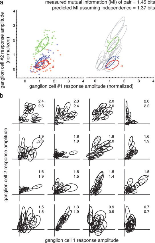
Calculation of mutual information for a pair of ganglion cells. a, Joint response amplitudes of ganglion cell 1 and ganglion cell 2. On the left, each point represents the magnitude of a single response to a flashed spot. Each point is colored (red, green, and blue) according to which stimulus spot (a, b, or c) was flashed. Response amplitudes are normalized by the mean response amplitude. Ellipses are drawn at 1 SD from the mean response to a given spot, and are the same spots shown in Figure 1. On the right, fits to the responses of the other 17 spots are shown (gray ellipses). The measured joint mutual information (top number) and predicted mutual information assuming independence of the responses of the two cells (bottom number) are shown. b, Gaussian fits of response distributions for 16 more cells. For each pair of cells, the actual (top number) and predicted mutual information assuming independence (bottom number) are shown. Cells are ordered from highest measured information (upper left) to lowest measured information.

All mutual information calculations were corrected for sampling bias by subtracting the mutual information obtained by randomly shuffling the responses with respect to the stimuli. The magnitude of the correction was 2.3 ± 0.1% of the total information for pairs of two cells and increased to 6.9 ± 0.05% for groups of 5 cells.

The error in each information quantity was estimated using a bootstrap resampling of the data. Random samples from the data, with replacement, were generated from the parameterized probability distribution and used to reestimate and recalculate the mutual information. These estimates yielded an average variance in the mutual information of ∼1%.

Mutual information curves from the data were compared with those obtained from a model in which the redundancy within a large population of neurons is uniformly distributed (Puchalla et al., 2005). In this model, the information I_n+1 of a population of n+1 neurons is given by the recursive relation:

where I_n is the information of n neurons and Δ is the pairwise redundancy. This model was fitted to the data allowing I₁ and Δ to vary.

Calculation of linear receptive fields and estimation of Gaussian receptive field model.

Flickering binary checkerboards were shown at 30 Hz for 15 min, and the fluctuations in intracellular current were recorded. Given the stimulus s(t) and the ganglion cell input current time course r(t), we calculated the linear kernel k(t) in the Fourier domain: F(ω) = R(ω)/S(ω), where F(ω), R(ω), and S(ω) are the Fourier transforms of f(t), r(t), and s(t). As the linear kernel f(t) was significantly nonzero in only a time window of duration t_f ∼1 s, we divided the data into M consecutive windows of length t_f, calculated F_i(ω) for each window, and took the inverse transform of the average F(ω) = 〈F_i(ω)〉_i (Press, 2007). Receptive fields were classified as inward, mixed or outward depending upon the shape of f(t).

The response amplitude of a given check was calculated by determining the principal components of the linear kernels over the central area of the checkerboard, using an analysis analogous to the analysis of responses to flashed spots, and then taking the dot product of each check's kernel with the first principal component. The typical raw response amplitude map was a 40 × 40 matrix.

For the two-dimensional Gaussian models of receptive fields, the raw response amplitude maps were fitted with two-dimensional Gaussians using a standard least-squares fitting algorithm to form a new, smoothed, Gaussian response map. In some cases, the map was resampled at lower resolution to improve convergence of the fitting algorithm. For the irregular receptive field models, the raw response amplitude maps were used, maintaining the irregularities that were otherwise smoothed away by the Gaussian fitting procedure.

The predicted amplitude of the response in the Gaussian model (i.e., the mean amplitude of the first principal component of the model response) was calculated by sampling the fitted two-dimensional Gaussian at the locations of the spots. For the irregular receptive field models, the predicted amplitude of the response was calculated by sampling the response amplitude map at the locations of the spots.

To better control the comparison between the model and actual data, the model responses were scaled by a proportionality factor chosen such that the entropy over all responses was equal to the measured entropy over all responses. A similar procedure was used in the irregular receptive field model. Noise was added to each of the model responses by adding Gaussian noise with SD calculated from the linear noise model for that cell (see Fig. 8a). A set of dummy trials the same size as the original dataset were generated.

Figure 8.

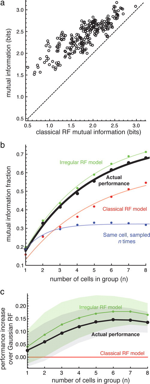
The measured performance of groups of ganglion cells is significantly higher than expected from a classical receptive field model. a, The measured performance of groups of five cells is plotted as a function of the predicted Gaussian receptive field model prediction. b, The mutual information fraction (mutual information divided by the total entropy of the stimulus) about the identity of the flashed spots conveyed by the responses of groups of ganglion cells is plotted as a function of the number of cells in the group. A value of 1 indicates that all 20 flashes could be identified without error. The black circles represent the performance measured for ganglion cells using flashed spots. The green, red, and blue circles represent the performance predicted from Gaussian, irregular, and complete overlap receptive field models, respectively. In all cases, the curve fitted to the points is the expected information if the pairwise redundancy is uniformly distributed over all of the pairs in a given group (see Materials and Methods). The data include groups composed of ganglion cells recorded simultaneously as well as groups composed of cells recorded at different times. c, The average difference in performance as a function of number of cells. Each point is the average of the difference between the actual performance (black points), the irregular RF model (green points), and the classical receptive field (RF) model. The shaded regions indicate ±1 SD.

Because the receptive field can contain both positive and negative components, negative response amplitudes are possible. It was assumed that the noise for negative response amplitudes was a constant and equal to the baseline noise. The results were not strongly dependent on this choice, as other models for the negative responses (i.e., noise proportional to the absolute value of the amplitude) gave similar results.

The spatial autocorrelation of receptive fields was calculated as the inverse Fourier transform of the two-dimensional spatial power spectrum of each receptive field radially sampled. Zero padding around the receptive field boundaries was used to minimize boundary effects, and the receptive field itself was divided into multiple overlapping subregions to reduce the noise in the power spectrum estimate (Press, 2007). The correlation caused by noise and discretization effects was subtracted by calculating the correlation function for receptive fields where the values were randomly resampled, and subtracting this correlation function from the total correlation; the correlation at larger distances was assumed to be zero. The one-dimensional correlation functions were fitted by least-squares minimization.

Results

We probed pieces of flat-mounted tiger salamander retina with a stimulus composed of 20 small spots flashed one at a time for 50 ms (Fig. 1a) at locations within a 200–300 μm diameter area, approximately equal to the size of a typical salamander ganglion cell's receptive field center (Segev et al., 2004). The responses were measured by whole-cell voltage clamp of pairs of ganglion cells located in the same region held near the Cl⁻ reversal potential (Fig. 1b). Spots were flashed 60 times each in random order on a rod-suppressing background. Their location, color, size and intensity were chosen to preferentially stimulate 1–2 long-wavelength-sensitive (L) cones at each location (see Materials and Methods).

We ask, given the responses of the ganglion cells, how well can one distinguish among the different spots, how does this performance depend upon the number of ganglion cells used, and what is the contribution of local irregularities, compared with the contribution of variations in receptive field position, size and orientation?

One possibility is that because the spots were all, nominally, within the center of the receptive fields of both ganglion cells, the responses of the two ganglion cells to all of the spots should be highly correlated. This would make the information encoded by the ganglion cells highly redundant. The responses of two ganglion cells are shown in Figure 1b. The flashes elicited a brief, rapidly increasing inward current, followed by a slower decay. The responses to different spots were not highly correlated between the two ganglion cells: spot B elicited large responses from both cells, while spots A and C elicited small responses from ganglion cell 1 and large responses from ganglion cell 2. Under these conditions, spots typically evoked short bursts of spikes in a current-clamped ganglion cell (Fig. 1c), and the magnitude of the input current response to a spot presented in a given location was approximately correlated with the number of spikes evoked by that spot (Fig. 1d).

The input current responses of a given ganglion cell were highly stereotyped, with most of the variation among responses accounted for by uniform scaling of the entire response waveform. We used principal components analysis to quantify this response (Fig. 2). Among all ganglion cells, the first principal component resembled the mean response and, on average, accounted for 94.3 ± 1.3% (mean ± SEM) of the signal variance. The second largest principal component captured, on average, 2.3 ± 0.6% of the signal variance, the third 1.0 ± 0.3%, with the remainder distributed among the remaining components. Because a large fraction of the variation was in the first principal component with very small contributions from all of the remaining components combined, the amplitude of a given response was defined as the projection of a given response waveform along the first principal component for that ganglion cell (see Materials and Methods).

If the responses of the ganglion cells were completely redundant, the joint responses of the two cells should be correlated and fall along a straight line in a plot of the second cell's response amplitude versus that of the first cell. However, many of the responses of this pair of cells deviated significantly from this pattern (Fig. 3a). Considerable decorrelation was observed in most of the recorded ganglion cell pairs (Fig. 3b). This suggests that despite the closeness of their cell bodies, the receptive fields of neighboring ganglion cells do not completely overlap. Whether this is caused by a gross difference in receptive field position and size or local irregularities within otherwise overlapping receptive fields is considered below.

Decorrelation should make the responses of neighboring ganglion cells more independent and allow more information to be represented by many cells. The independence of visual encoding can be calculated using the mutual information between stimulus and response, i.e., how much information is conveyed by the responses about which of the 20 spots was flashed. If two ganglion cells convey information independently, the information about the stimulus calculated from the joint response should be equal to the sum of the mutual information of each ganglion cell taken alone. For this pair of cells, the joint mutual information (1.45 ± 0.05 bits, mean ± SEM) was slightly higher than expected if the cells signaled independently (1.37 ± 0.05 bits, Fig. 3a), indicating that the pair signals slightly synergistically. The pair conveys a substantial fraction (34%) of the maximum possible information about spot location (log₂ 20 ∼4.3 bits).

The signaling among most ganglion cell pairs was nearly independent, i.e., the measured mutual information for ganglion cells pairs fell close to that predicted by summing the information of each ganglion cell taken alone (Fig. 4). Simultaneously recorded pairs (black points) and pairs recorded at different times but from the same patch of retina (gray points) were distributed similarly, suggesting that the contribution of correlated trial-by-trial variation (noise correlation) was small. The majority of pairs fell slightly below the unity line (Fig. 4, coarse dashed line) with slope 0.95 (solid lines), indicating that the signaling among pairs was mildly redundant, close to the 10% redundancy reported previously for spikes trains from pairs of ganglion cells under naturalistic stimulation (Puchalla et al., 2005).

Figure 4.

Most ganglion cell pairs signal nearly independently. The mutual information for a pair of ganglion cells is plotted as function of the predicted mutual information assuming independence. The coarse dashed line has slope 1, the fine dashed line has slope 0.5. The black points are pairs of ganglion cells recorded simultaneously and the gray points are pairs recorded at different times but in response to the same set of spots. Error bars are the estimated SD of the mutual information value, calculated by bootstrap (see Materials and Methods). The slope of the best-fit line to each population is drawn (solid lines). The cyan arrowhead indicates the one example in which the cell pair was redundant as expected from noise alone. The red arrowhead indicates the cell pair shown in Figure 3a.

One possible explanation for the near-independence of ganglion cell signaling is that the relatively low redundancy was due to noise, which, if large enough, would have caused the responses of ganglion cells to be independent. To assess the contribution of noise, we calculated the mutual information for a synthetic pair composed of a single cell sampled twice—the equivalent of two cells with completely overlapping receptive fields but independent noise (Fig. 4, blue points). If there were no noise in the system, these points would lie along the line of slope 0.5 (fine dashed line). As expected, noise causes the responses to be more independent, but does not account for the near-independence of most ganglion cell pairs. Of the 105 pairs shown, only one ganglion cell pair was as redundant as expected from completely overlapping receptive fields (Fig. 4, cyan arrowhead). The near independence of ganglion cell pairs is therefore the result of genuine differences in spatial sampling, not noise in retinal circuitry.

We divided our ganglion cell population into three functional types based on their reverse correlation to flickering checkerboard stimulation—those in which an increase in light intensity caused an inward, outward or mixed current response (Fig. 5a). There was no significant difference in the information encoded among the three functional classes (Fig. 5b) (e.g., inward vs outward, p = 0.14 by Kolmogorov–Smirnov test). There was no significant difference in the mean independence among pairs composed of different types (Fig. 5c), with the exception of outward-outward pairs, which were more redundant, signaling with 90% independence compared with the 94–99% independence of the other pairs. These results indicate that under our stimulus and recording conditions, information about the location of small flashed spots was distributed widely within the ganglion cell population and represented in a similar fashion by different cell types. Because of this similarity, we pooled results across cell types in the remainder of the paper. It is certainly possible that under different stimulus conditions, light responses may differ more markedly among cell types.

Figure 5.

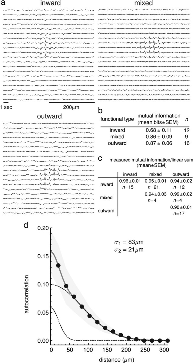
Analysis of receptive field spatial autocorrelation and information among cell types. a, Examples of inward-, mixed-, and outward-type receptive fields. For clarity, each trace represents the average linear filter waveform of the 2 × 2 underlying linear filters, so while each original check was 20 × 20 μm, the filters are the average over a 40 × 40 μm area. A negative peak in the filter means that an increase in light intensity causes an inward, or excitatory current in the cell. b, Mean single cell mutual information for the three cell types. c, Ratio between measured mutual information of the pair and the expected mutual information assuming independence (linear sum). d, Spatial autocorrelation function for measured receptive fields. The data from cells of all types are combined. The gray region indicates the SEM of the mean autocorrelation function. The thick gray line is the sum of two Gaussian functions used to fit the data, and the dashed lines are each of the two functions taken individually. The SD σ of the wider (σ₁) and narrower (σ₂) Gaussians are reported (note that the 1/e width of the Gaussian is 2σ).

To characterize the local irregularities in our receptive fields, the spatial autocorrelation function of the receptive field was calculated, taking into account the autocorrelation due to the size of the checkerboard squares (20 μm, for details see Materials and Methods). The width of this function summarizes the typical size of spatial variations in the sensitivity of the receptive field. The spatial autocorrelation function was well described by the sum of two Gaussian profiles with half-widths of 21 and 83 μm (Fig. 5d). There was no significant difference in the fit among the three functional cell types (data not shown). The smaller width is comparable to the spacing between cone photoreceptors (∼20 μm), and the larger is consistent with the range of receptive field center diameters (∼100–400 μm) reported in salamander (Segev et al., 2004).

In retinal mosaics, variability in the position and size of receptive fields can have a substantial effect on the representation of spatial detail (Liu et al., 2009). To measure this contribution in groups of ganglion cells with highly overlapping receptive fields, the measured receptive field of each ganglion cell was fitted with a two-dimensional Gaussian (Fig. 6; Materials and Methods). The fitted receptive fields were on average 203 ± 107 μm in diameter with average long/short axis ratio of 1.5, consistent with receptive fields generated from spike-triggered averages (Segev et al., 2004). This diameter approximately matched the wider component of the spatial autocorrelation function (Fig. 5d). Local irregularities can be seen as peaks and valleys in the sensitivity profile of individual ganglion cells, which are not captured by a Gaussian fit (Fig. 6c).

Figure 6.

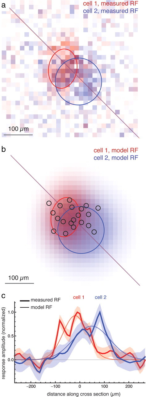
Receptive field measurement and fitting with Gaussian receptive field model. a, Two-dimensional receptive field map for two ganglion cells (red and blue) with sensitivity represented on an intensity scale. Ellipses are the 1 SD boundaries for the fitted Gaussian receptive field model; cross section in c is shown with a line. Cell 1 is mixed type and Cell 2 is outward type. b, Fitted Gaussian receptive fields of the same two cells. Black circles indicate location and size of flashed spots. c, Cross section of receptive field along a single spatial axis (indicated by diagonal line in a and b). Thick line is the measured receptive field, thin line is the fitted Gaussian receptive field, and shaded area is ±1 SEM. Cross sections are normalized by their maximum amplitude.

Next, we tested whether the receptive field model could account for the actual coding performance of ganglion cells in the flashed-spot experiment. Because the mutual information depends both on signal and noise, we needed to have a model of the noise in the response, i.e., how the variability in a response to a given spot depended on the mean amplitude of the response to that spot. For nearly all ganglion cells, the measured noise increased approximately linearly with mean signal amplitude with a slope in the range of 0.1–0.3 atop a relatively small constant background noise (Fig. 7a). Thus, we assumed that the average response to a small flash was proportional to the Gaussian receptive field amplitude at the location of the spot and that the noise was linearly related to this signal. For each cell, the slope and offset of the fitted line was used to calculate the expected SD of the noise in the response for a given response amplitude. The slope of the noise model was not significantly correlated among cells, whether recorded at the same time or in the same location (Fig. 7b; Pearson correlation, r = 0.039).

Figure 7.

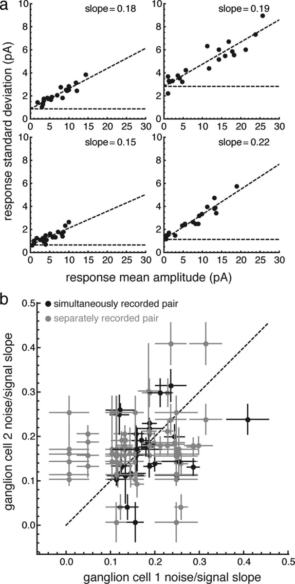
Noise in retinal ganglion cells increases approximately linearly with a different characteristic slope for each ganglion cell. a, Each panel represents one ganglion cell. Each point represents the mean and SD of the responses to 1 of 20 spots. The data are fitted with a model in which the noise increases linearly with the indicated slope (dashed line). b, The noise slope is plotted for pairs of cells recorded simultaneously (black points) and on separate trials (gray points).

Despite taking into account the positions and sizes of the receptive fields, and controlling for differences in noise among individual cells, the Gaussian receptive field model could not account for a substantial fraction of the information represented by the ganglion cells. For groups composed of five cells, the observed responses conveyed 33% more information than the matched, Gaussian receptive field model (2.4 ± 0.3 bits compared with 1.8 ± 0.5 bits, Fig. 8a). Furthermore, the actual performance was more consistent: although the Gaussian model predicted that many groups would encode <12% of the information about spot location, the actual performance fell within a smaller range, with groups never encoding <34% and at best encoding 81% of the information.

As expected, as more ganglion cells were considered, the information about the stimulus increased (Fig. 8b). The increase was more rapid, however, for the measured data than the Gaussian model. Groups of eight ganglion cells on average encoded 68.0 ± 0.4% of the information; in comparison, model cells encoded only 54.5 ± 0.7% of the information. The increases in all cases were explained by a simple model in which the observed pairwise redundancy is uniformly distributed among all of the cells in the group (Puchalla et al., 2005) (Fig. 8b, solid lines) (see Materials and Methods). This suggests that pairwise interactions are the dominant source of redundancy, as found in more complex stimulus conditions (Schneidman et al., 2006; Shlens et al., 2009).

Pairwise decorrelation is potentially a strong effect because the number of pairwise interactions increases quadratically with the number of cells in a group, and a modest decrease in pairwise redundancy can cause a large increase in the information conveyed by the entire group. Consistent with this prediction, the actual spatial information encoded was significantly higher for the responses of real ganglion cells than that predicted by the classical model for a groups as small as n = 2 (p = 0.0016).

In models of retinal mosaics, most of the increase in mutual information between stimulus and response occurred when the size and orientation of receptive fields were optimized to compensate for irregularities in the lattice itself (Liu et al., 2009). Further optimization of the receptive field boundaries by adding non-Gaussian distortions had a relatively weak effect. In contrast, in our experiments with groups of ganglion cells with highly overlapping receptive fields, local irregularities caused an improvement nearly as large or larger than the improvement caused by deoverlapping the receptive fields and allowing them to have differing size and shape. That is, the difference between the actual performance (Fig. 8b, black line) and the Gaussian model (Fig. 8b, red line) is nearly as great or greater than the difference between the Gaussian model and the case of n perfectly overlapping cells (Fig. 8b, blue line).

One possible explanation for the poor performance of the Gaussian receptive field model is that it is somehow handicapped by bias in the receptive field fitting procedure, reducing its coding capacity. In this comparison, however, the entropy of a single model cell's response was constrained to be the same as in the measured data (see Materials and Methods), so that the coding capacity of a single model cell was equal with respect to the stimulus. The differences in signaling are thus due to differences in receptive field overlap, not the coding capacity of individual cells.

The actual performance was explained, however, if local irregularities in each cell's spatial receptive field profile were taken into account. Another receptive field model was constructed by generating responses proportional to the actual sensitivity at the spot location, rather than the Gaussian approximation (for details, see Materials and Methods). The irregular receptive field model more closely predicted the actual performance (Fig. 8b, green points).

Discussion

Previous studies using spike-triggered averages have focused upon how visual information is represented by retinal mosaics composed of a single type of ganglion cell with little receptive field overlap (Wässle and Boycott, 1991; Borghuis et al., 2008; Gauthier et al., 2009; Shlens et al., 2009). The local irregularities that we report here are consistent with recent studies in the macaque retina (Field et al., 2010) in which receptive fields measured at the single cone level also appeared punctate and non-Gaussian. We find here that local irregularities in the receptive fields have a large effect on the representation of spatial information in the input currents of heterogeneous groups of ganglion cells with highly overlapping receptive fields. For the group sizes examined here, fine irregularities increased the total information represented in the input currents by up to 33%. In comparison, in a nonoverlapping retinal mosaic, small perturbations in the receptive field boundary caused the performance on a spatial localization task to increase by 3% (Liu et al., 2009).

While the spiking output generally correlates with the amplitude of the input currents under these stimulus conditions (Fig. 1c,d), it will be interesting to determine whether this additional information represented by the inner retina is ultimately preserved in the spiking output of retinal ganglion cells. The nonlinearity of spike generation could transform the input we measured from the inner retina to extract certain features, but ultimately lose some of the mutual information between spatial location and output. The transmission of spatial information across the spiking nonlinearity might also depend on the context of the rest of the image. A single small spot might induce a current too small to drive a spike, but the presentation of the same spot along with the illumination of other regions in a ganglion cell receptive field that add their own excitatory drive, might modulate the firing rate.

Anatomical and physiological evidence suggest that information from mixed ganglion cell types converge in higher visual processing areas. Because of this convergence, it is important to characterize the spatial information encoded by mixed populations of ganglion cells. Retinal ganglion cells project to different brain regions, but the major projection sites—the dorsal lateral geniculate nucleus and superior colliculus (SC) in mammals—both receive inputs from many ganglion cell types (Berson, 2008). In particular, the SC in mammals receives input from almost every ganglion cell type, with the most notable exceptions being β cells in the cat and midget cells in the monkey (Stone, 1983; Tamamaki et al., 1995; Rodieck, 1998). Similar results have been reported for projections to the contralateral optic tectum in the salamander (Roth, 1987; Wiggers, 1999). This implies that spatial information from multiple ganglion cell types can be integrated by the central brain. Retinal fibers from different cell types arborize in different lamina of the SC (Huberman et al., 2008, 2009; Kim et al., 2010), allowing for specialized processing. However, dendrites of some collicular neurons span all the retinal input layers (Roth, 1987; Shlens et al., 2006), implying that even single neurons can integrate information from all ganglion cell types.

Local irregularities in ganglion cell receptive fields have been noted since the earliest measurements of receptive fields in the retina (Kuffler, 1953). There are two reasons that local irregularities have not been more carefully examined until recently. First, they are obscured by commonly used methods of measuring and characterizing receptive fields. Consistent with this explanation, we found that the spatial autocorrelation of the receptive fields revealed a length scale of ∼20 μm at which fine irregularities appeared. These local irregularities will be blurred by coarse checkerboards (Segev et al., 2004) or spots, bars or gratings larger than ∼20 μm. Indeed, studies using high spatial frequency gratings in macaque retina found that the parvocellular pathway cells were often bimodal in shape, consistent with local patchiness or irregularities (Passaglia et al., 2002).

Second, local irregularities are expected to play a small role in encoding in mosaics with 1SD receptive field spacing because of the Nyquist sampling limit—spatial features of smaller than the receptive field spacing are poorly represented in the encoding to begin with, so local irregularities would be expected to affect the overall performance relatively little. This was the result found by Liu et al. for the case of introducing fluctuations in receptive field boundaries, which are features smaller than the Nyquist sampling limit (Liu et al., 2009).

However, in highly overlapping receptive field mosaics the Nyquist sampling limit is much higher. Fine spatial irregularities will tend to orthogonalize the sampling of overlapping receptive fields so that sampling at higher spatial frequencies more closely approaches the Nyquist limit, increasing the information encoded by the mosaic. As we show here, this effect can be large among small groups of cells. It is important, however, to consider that the nonuniformity caused by spatial irregularities also degrades performance compared with perfectly uniform sampling. The degree of degradation depends upon the degree of correlation of fine spatial irregularities among different cells. If the irregularities are statistically independent, then the amplitude of the nonuniformity in sampling will be small due to averaging among the cells, which for salamander retina would cause the overall nonuniformity to be ∼√60 times smaller than the irregularity in a single cell (Segev et al., 2004). If the locations perfectly coincide, the amplitude of the nonuniformity will be on the order of that of an individual cell. Given that the irregularities in single cells that we observe here are of the order of ∼10% of the sensitivity, the degradation of performance due to nonuniformity are expected to be relatively small in either case. We caution, however, that without knowing the correlation between irregularities among all of the cells sampling a patch of retina, it is not possible to say for sure how these competing effects trade-off overall.

Local irregularities could be generated by nonuniform sampling from individual bipolar cells. However, this is not consistent with existing measurements of the bipolar receptive field size, which vary widely: 50–150 μm measured using reverse correlation (Baccus et al., 2008), 62 and 124 μm for ON and OFF center bipolar cells, respectively, measured using spots of increasing radius (Hare and Owen, 1990), and 300–500 μm measured using a 100 μm bar (Zhang and Wu, 2009). One possibility is that there is a class of bipolar cell with very small receptive fields (∼40 μm across) that makes synapses onto ganglion cells with highly nonuniform strength. Another possibility is that bipolar cells themselves have local irregularities within their receptive fields. This property has not been reported, but we are not aware of any high-resolution measurements that could test this hypothesis. A final possibility is that the rectification nonlinearity found in many bipolar-to-ganglion cell synapses can impose a threshold that restricts the spatial region in the bipolar receptive field that effectively drives glutamate release and thus results in spatially localized “hot spots.”

To explore how spatial information is arranged among different kinds of ganglion cells, we divided our sample into three major functional types (inward, outward, and mixed) based on reverse correlation to a flickering checkerboard. We found that the degree of pairwise redundancy in the input currents did not depend strongly on the functional type of the cell or on whether cells were of the same type (except for outward-outward pairs, which were ∼10% redundant). This result is similar to previous measurements of the redundancy between spike trains of ganglion cells of different functional types, despite the fact that the stimuli were very different (flashed spots vs natural movie clips) (Segev et al., 2006). This comparison supports the view that ganglion cells in the salamander retina have a broad spectrum of functional properties.

Our analysis of the three functional classes that we observed (inward, mixed and outward) is meant to show that fine spatial information is broadly distributed within the ganglion cell population—not to make a direct comparison to classical cell types in the retina. While it is intuitive to identify cells having an inward current with ON cells and outward current with OFF cells, the detailed correspondence is not so straightforward. Because in our measurements the cell is voltage-clamped near, but not precisely at the inhibitory reversal potential, the responses measured here may be caused by a mix of inward and outward currents. Without a more detailed analysis at several holding potentials, it is not possible to say whether an outward current is due to an in an inhibitory current, or by a sustained excitation that is transiently shut off, perhaps by presynaptic inhibition. In classical measurements, which are done in current clamp or extracellularly, both excitatory and inhibitory currents contribute to the spiking activity and underlying swings in membrane potential. For these reasons, we caution against any direct comparison between the functional types that we observe here and cell types measured by other means.

A previous study analyzed the redundancy between ganglion cell spike trains during stimulation with natural movie clips (Puchalla et al., 2005). This study estimated that the total redundancy in the ganglion cell population was ∼10-fold, much larger than found in the present study. However, this estimate involved populations of 200+ cells. When we instead compare pairwise redundancy, we find more similar results: an average redundancy of ∼10% for spike trains during natural movies vs ∼5% for input currents evoked by flashed spots. Because the visual stimuli were not the same in the two studies, one does not expect exactly the same results. Instead, the rough similarity of the two results suggests that input currents encode information in a similar fashion to spike trains. Furthermore, the “uniformity” assumption used to derive the estimate of tenfold population redundancy (Puchalla et al., 2005) appears to be closely obeyed in the current data (Fig. 8b).

Nearly independent encoding in cells with similar stimulus selectivity has been observed elsewhere in the visual system. In primary visual cortex, deviations from the classical Gabor structure of a simple cell receptive field, as well as irregularities in the receptive field position, size and orientation (DeAngelis et al., 1999; Ringach et al., 2002) are well documented. The same is true for complex cells (Ringach et al., 1997). Cells in primary visual cortex have been shown to encode information nearly independently despite considerable receptive field overlap (Reich et al., 2001). It has also been demonstrated theoretically that a group of neurons with tuning curve diversity can add information independently as opposed to a population with homogeneous tuning in which the information encoded by the population saturates (Shamir and Sompolinsky, 2006).

While local irregularities in ganglion cell receptive field structure may seem like a defect in the construction of the retinal circuitry, our data suggest that the retina and the brain may take direct advantage of these irregularities to sample small regions of visual space. At first glance, a distributed code based upon receptive fields with local irregularities may appear more complex, as the information about fine spatial detail requires a readout circuit with weights tuned to capture the irregularities. This is also true, however, of an irregularly spaced lattice with receptive fields that vary in shape and orientation. As we show here, a distributed code can be more efficient than expected from classical receptive field models. In addition, the developmental mechanisms required to generate irregular, decorrelated receptive fields—random sampling and local interactions—may also be simpler and more robust than those required to generate perfectly regular, smooth arrays.

References

- Atick JJ, Redlick AN. Towards a theory of early visual processing. Neural Comput. 1990;2:308–320. [Google Scholar]
- Baccus SA, Olveczky BP, Manu M, Meister M. A retinal circuit that computes object motion. J Neurosci. 2008;28:6807–6817. doi: 10.1523/JNEUROSCI.4206-07.2008. [DOI] [PMC free article] [PubMed] [Google Scholar]
- Berson DM. Retinal ganglion cell types and their central projections. In: Basbaum AI, Bushnell MC, Smith DV, Beauchamp GK, Firestein SJ, Dallos P, Oertel D, Masland RH, Albright T, Kaas JH, Gardner EP, editors. The senses: a comprehensive reference. New York: Elsevier; 2008. pp. 491–519. [Google Scholar]
- Borghuis BG, Ratliff CP, Smith RG, Sterling P, Balasubramanian V. Design of a neuronal array. J Neurosci. 2008;28:3178–3189. doi: 10.1523/JNEUROSCI.5259-07.2008. [DOI] [PMC free article] [PubMed] [Google Scholar]
- Brown SP, He S, Masland RH. Receptive field microstructure and dendritic geometry of retinal ganglion cells. Neuron. 2000;27:371–383. doi: 10.1016/s0896-6273(00)00044-1. [DOI] [PubMed] [Google Scholar]
- Dacey DM, Peterson BB, Robinson FR, Gamlin PD. Fireworks in the primate retina: in vitro photodynamics reveals diverse LGN-projecting ganglion cell types. Neuron. 2003;37:15–27. doi: 10.1016/s0896-6273(02)01143-1. [DOI] [PubMed] [Google Scholar]
- DeAngelis GC, Ghose GM, Ohzawa I, Freeman RD. Functional micro-organization of primary visual cortex: receptive field analysis of nearby neurons. J Neurosci. 1999;19:4046–4064. doi: 10.1523/JNEUROSCI.19-10-04046.1999. [DOI] [PMC free article] [PubMed] [Google Scholar]
- Devries SH, Baylor DA. Mosaic arrangement of ganglion cell receptive fields in rabbit retina. J Neurophysiol. 1997;78:2048–2060. doi: 10.1152/jn.1997.78.4.2048. [DOI] [PubMed] [Google Scholar]
- Field GD, Gauthier JL, Sher A, Greschner M, Machado TA, Jepson LH, Shlens J, Gunning DE, Mathieson K, Dabrowski W, Paninski L, Litke AM, Chichilnisky EJ. Functional connectivity in the retina at the resolution of photoreceptors. Nature. 2010;467:673–677. doi: 10.1038/nature09424. [DOI] [PMC free article] [PubMed] [Google Scholar]
- Gauthier JL, Field GD, Sher A, Greschner M, Shlens J, Litke AM, Chichilnisky EJ. Receptive fields in primate retina are coordinated to sample visual space more uniformly. PLoS Biol. 2009;7:e1000063. doi: 10.1371/journal.pbio.1000063. [DOI] [PMC free article] [PubMed] [Google Scholar]
- Hare WA, Owen WG. Spatial organization of the bipolar cell's receptive field in the retina of the tiger salamander. J Physiol. 1990;421:223–245. doi: 10.1113/jphysiol.1990.sp017942. [DOI] [PMC free article] [PubMed] [Google Scholar]
- Huberman AD, Manu M, Koch SM, Susman MW, Lutz AB, Ullian EM, Baccus SA, Barres BA. Architecture and activity-mediated refinement of axonal projections from a mosaic of genetically identified retinal ganglion cells. Neuron. 2008;59:425–438. doi: 10.1016/j.neuron.2008.07.018. [DOI] [PMC free article] [PubMed] [Google Scholar]
- Huberman AD, Wei W, Elstrott J, Stafford BK, Feller MB, Barres BA. Genetic identification of an On-Off direction-selective retinal ganglion cell subtype reveals a layer-specific subcortical map of posterior motion. Neuron. 2009;62:327–334. doi: 10.1016/j.neuron.2009.04.014. [DOI] [PMC free article] [PubMed] [Google Scholar]
- Kim IJ, Zhang Y, Meister M, Sanes JR. Laminar restriction of retinal ganglion cell dendrites and axons: subtype-specific developmental patterns revealed with transgenic markers. J Neurosci. 2010;30:1452–1462. doi: 10.1523/JNEUROSCI.4779-09.2010. [DOI] [PMC free article] [PubMed] [Google Scholar]
- Kim KJ, Rieke F. Temporal contrast adaptation in the input and output signals of salamander retinal ganglion cells. J Neurosci. 2001;21:287–299. doi: 10.1523/JNEUROSCI.21-01-00287.2001. [DOI] [PMC free article] [PubMed] [Google Scholar]
- Kim KJ, Rieke F. Slow Na+ inactivation and variance adaptation in salamander retinal ganglion cells. J Neurosci. 2003;23:1506–1516. doi: 10.1523/JNEUROSCI.23-04-01506.2003. [DOI] [PMC free article] [PubMed] [Google Scholar]
- Kuffler SW. Discharge patterns and functional organization of mammalian retina. J Neurophysiol. 1953;16:37–68. doi: 10.1152/jn.1953.16.1.37. [DOI] [PubMed] [Google Scholar]
- Liu YS, Stevens CF, Sharpee TO. Predictable irregularities in retinal receptive fields. Proc Natl Acad Sci U S A. 2009;106:16499–16504. doi: 10.1073/pnas.0908926106. [DOI] [PMC free article] [PubMed] [Google Scholar]
- Ma J, Znoiko S, Othersen KL, Ryan JC, Das J, Isayama T, Kono M, Oprian DD, Corson DW, Cornwall MC, Cameron DA, Harosi FI, Makino CL, Crouch RK. A visual pigment expressed in both rod and cone photoreceptors. Neuron. 2001;32:451–461. doi: 10.1016/s0896-6273(01)00482-2. [DOI] [PubMed] [Google Scholar]
- Makino CL, Taylor WR, Baylor DA. Rapid charge movements and photosensitivity of visual pigments in salamander rods and cones. J Physiol. 1991;442:761–780. doi: 10.1113/jphysiol.1991.sp018818. [DOI] [PMC free article] [PubMed] [Google Scholar]
- Passaglia CL, Troy JB, Rüttiger L, Lee BB. Orientation selectivity of ganglion cells in primate retina. Vision Res. 2002;42:683–694. doi: 10.1016/s0042-6989(01)00312-1. [DOI] [PMC free article] [PubMed] [Google Scholar]
- Pillow JW, Shlens J, Paninski L, Sher A, Litke AM, Chichilnisky EJ, Simoncelli EP. Spatio-temporal correlations and visual signalling in a complete neuronal population. Nature. 2008;454:995–999. doi: 10.1038/nature07140. [DOI] [PMC free article] [PubMed] [Google Scholar]
- Press WH. Cambridge, UK: Cambridge UP; 2007. Numerical recipes: the art of scientific computing. [Google Scholar]
- Puchalla JL, Schneidman E, Harris RA, Berry MJ. Redundancy in the population code of the retina. Neuron. 2005;46:493–504. doi: 10.1016/j.neuron.2005.03.026. [DOI] [PubMed] [Google Scholar]
- Reich DS, Mechler F, Victor JD. Independent and redundant information in nearby cortical neurons. Science. 2001;294:2566–2568. doi: 10.1126/science.1065839. [DOI] [PubMed] [Google Scholar]
- Ringach DL, Hawken MJ, Shapley R. Dynamics of orientation tuning in macaque primary visual cortex. Nature. 1997;387:281–284. doi: 10.1038/387281a0. [DOI] [PubMed] [Google Scholar]
- Ringach DL, Shapley RM, Hawken MJ. Orientation selectivity in macaque V1: diversity and laminar dependence. J Neurosci. 2002;22:5639–5651. doi: 10.1523/JNEUROSCI.22-13-05639.2002. [DOI] [PMC free article] [PubMed] [Google Scholar]
- Rodieck RW. Quantitative analysis of cat retinal ganglion cell response to visual stimuli. Vision Res. 1965;5:583–601. doi: 10.1016/0042-6989(65)90033-7. [DOI] [PubMed] [Google Scholar]
- Rodieck RW. Sunderland, MA: Sinauer Associates; 1998. The first steps in seeing. [Google Scholar]
- Roth G. Berlin: Springer; 1987. Visually guided behavior in salamanders. [Google Scholar]
- Schneidman E, Berry MJ, 2nd, Segev R, Bialek W. Weak pairwise correlations imply strongly correlated network states in a neural population. Nature. 2006;440:1007–1012. doi: 10.1038/nature04701. [DOI] [PMC free article] [PubMed] [Google Scholar]
- Segev R, Goodhouse J, Puchalla J, Berry MJ., 2nd Recording spikes from a large fraction of the ganglion cells in a retinal patch. Nat Neurosci. 2004;7:1154–1161. doi: 10.1038/nn1323. [DOI] [PubMed] [Google Scholar]
- Segev R, Puchalla J, Berry MJ., 2nd Functional organization of ganglion cells in the salamander retina. J Neurophysiol. 2006;95:2277–2292. doi: 10.1152/jn.00928.2005. [DOI] [PubMed] [Google Scholar]
- Shamir M, Sompolinsky H. Implications of neuronal diversity on population coding. Neural Comput. 2006;18:1951–1986. doi: 10.1162/neco.2006.18.8.1951. [DOI] [PubMed] [Google Scholar]
- Shlens J, Field GD, Gauthier JL, Grivich MI, Petrusca D, Sher A, Litke AM, Chichilnisky EJ. The structure of multi-neuron firing patterns in primate retina. J Neurosci. 2006;26:8254–8266. doi: 10.1523/JNEUROSCI.1282-06.2006. [DOI] [PMC free article] [PubMed] [Google Scholar]
- Shlens J, Field GD, Gauthier JL, Greschner M, Sher A, Litke AM, Chichilnisky EJ. The structure of large-scale synchronized firing in primate retina. J Neurosci. 2009;29:5022–5031. doi: 10.1523/JNEUROSCI.5187-08.2009. [DOI] [PMC free article] [PubMed] [Google Scholar]
- Stone J. New York: Plenum; 1983. Parallel processing in the visual system: the classification of retinal ganglion cells and its impact on the neurobiology of vision. [Google Scholar]
- Tamamaki N, Uhlrich DJ, Sherman SM. Morphology of physiologically identified retinal X and Y axons in the cat's thalamus and midbrain as revealed by intraaxonal injection of biocytin. J Comp Neurol. 1995;354:583–607. doi: 10.1002/cne.903540408. [DOI] [PubMed] [Google Scholar]
- Wässle H, Boycott BB. Functional architecture of the mammalian retina. Physiol Rev. 1991;71:447–480. doi: 10.1152/physrev.1991.71.2.447. [DOI] [PubMed] [Google Scholar]
- Wiggers W. Projections of single retinal ganglion cells to the visual centers: an intracellular staining study in a plethodontid salamander. Vis Neurosci. 1999;16:435–447. doi: 10.1017/s0952523899163053. [DOI] [PubMed] [Google Scholar]
- Zhang AJ, Wu SM. Receptive fields of retinal bipolar cells are mediated by heterogeneous synaptic circuitry. J Neurosci. 2009;29:789–797. doi: 10.1523/JNEUROSCI.4984-08.2009. [DOI] [PMC free article] [PubMed] [Google Scholar]