QuShape: Rapid, accurate, and best-practices quantification of nucleic acid probing information, resolved by capillary electrophoresis

Chemical probing of RNA and DNA structure is a widely used and highly informative approach for examining nucleic acid structure and for evaluating interactions with protein and small-molecule ligands. QuShape, described in this paper, is a platform-independent, user-friendly software package that yields quantitative and objective nucleotide reactivity information as resolved by automated high-throughput capillary electrophoresis instruments.

Abstract

Chemical probing of RNA and DNA structure is a widely used and highly informative approach for examining nucleic acid structure and for evaluating interactions with protein and small-molecule ligands. Use of capillary electrophoresis to analyze chemical probing experiments yields hundreds of nucleotides of information per experiment and can be performed on automated instruments. Extraction of the information from capillary electrophoresis electropherograms is a computationally intensive multistep analytical process, and no current software provides rapid, automated, and accurate data analysis. To overcome this bottleneck, we developed a platform-independent, user-friendly software package, QuShape, that yields quantitatively accurate nucleotide reactivity information with minimal user supervision. QuShape incorporates newly developed algorithms for signal decay correction, alignment of time-varying signals within and across capillaries and relative to the RNA nucleotide sequence, and signal scaling across channels or experiments. An analysis-by-reference option enables multiple, related experiments to be fully analyzed in minutes. We illustrate the usefulness and robustness of QuShape by analysis of RNA SHAPE (selective 2′-hydroxyl acylation analyzed by primer extension) experiments.

INTRODUCTION

Chemical probing of RNA and DNA at single-nucleotide resolution is a highly effective strategy for characterizing structure–function relationships. Chemical probing approaches are widely used to develop secondary and tertiary structure models, to identify molecular and protein ligand interaction sites, to characterize conformational changes, and to examine other functional properties of nucleic acids (Nielsen 1990; Weeks 2010). Chemical probing of RNA structure has become especially important with the realization that much of the information expressed in RNA is encoded in the form of complex higher-order structures. In the SHAPE (selective 2′-hydroxyl acylation analyzed by primer extension) technologies, an RNA is reacted with an electrophilic reagent that can form an adduct with ribose 2′-OH groups in a manner dependent on the conformational flexibility of each nucleotide (Fig. 1A; Merino et al. 2005; Gherghe et al. 2008; McGinnis et al. 2012). Sites in the RNA that form 2′-O-adducts can be detected as stops to reverse transcriptase–mediated primer extension (Fig. 1B) that can be visualized by high-throughput capillary electrophoresis (Fig. 1C; Wilkinson et al. 2008; McGinnis et al. 2009; Watts et al. 2009). SHAPE reactivities correlate strongly with model-free measurements of molecular order and are largely independent of nucleotide type or solvent accessibility (Gherghe et al. 2008; Wilkinson et al. 2009; McGinnis et al. 2012). SHAPE reactivity information has been used to develop RNA secondary structure models, to detect changes in RNA conformation, and to monitor interactions with proteins, ligands, and metal ions.

FIGURE 1.

SHAPE chemical probing of RNA structure. (A) Mechanism of SHAPE chemistry. (B) Extension of fluorescently labeled primers by reverse transcriptase from the 3′ end of an RNA to the site of the first adduct generates a population of fluorescently labeled cDNA molecules. (C) Capillary electrophoresis yields an electropherogram trace that quantitatively reflects cDNA molecules of various lengths, thus indicating the positions of flexible nucleotides in the RNA molecule.

It has been a challenge to read out SHAPE reactivity information, or the results of any nucleic acid probing experiment, efficiently and accurately. The current gold standard for accurately detecting and quantifying the sites of 2′-O-adduct formation makes use of capillary electrophoresis (CE) electropherograms. Extracting quantitative reactivities for each nucleotide requires extensive multistep analytical signal processing. Diverse software tools have been developed to facilitate processing of electropherograms, including CAFA (Mitra et al. 2008), ShapeFinder (Vasa et al. 2008), HiTRACE (Yoon et al. 2011), FAST (Pang et al. 2011), and SHAPE-CE (Aviran et al. 2011b). There is a critical balance to be struck between processing speed, pipeline simplicity, and degree of automation. For example, some high-throughput processing approaches yield sequence misalignments and integration errors (as reported by Leonard et al. 2012; Ritz et al. 2012). The ShapeFinder package (Vasa et al. 2008) is the most widely used among current software tools and ultimately yields final data sets of high quality. However, to achieve a high level of quantitative accuracy, ShapeFinder requires the user to manually select tools and associated parameters at many data analysis steps, making data processing laborious and time consuming. Judgment calls are often necessary, making data analysis nonobjective and requiring significant user training.

With the goal of achieving both automation and high levels of accuracy, we have created optimized computational approaches for streamlined and comprehensive analysis of experimental high-throughput SHAPE-CE data. These algorithms are implemented in a platform-independent, user-friendly software package called QuShape () to yield objective nucleotide reactivity information with minimal user supervision.

Principles of SHAPE-based chemical probing of RNA structure

A current-generation SHAPE experiment involves four steps (Vasa et al. 2008; Wilkinson et al. 2008). First, RNA is treated with an electrophilic reagent that reacts selectively with the 2′-OH group of conformationally flexible RNA nucleotides (Fig. 1A). Second, sites of RNA modification are scored as stops to reverse transcriptase–mediated primer extension using labeled DNA primers (Fig. 1B). The products of this primer extension reaction are 5′-end-labeled cDNA fragments with lengths that correspond to the modified positions in the RNA. As a control, a primer extension reaction is also performed on RNA not treated with the reagent. In addition, dideoxynucleotide (ddNTP) sequencing reactions are performed and used to assign observed reactivities to the RNA nucleotide sequence. Primers are labeled with different color-coded fluorophores to distinguish modification, control, and sequencing reactions. Third, the primer extension reactions are resolved in one or more capillaries on a capillary electrophoresis instrument (Fig. 1C). Finally, the resulting CE electropherograms are subjected to signal processing to align all peaks with each other and to the known RNA sequence with the goal of calculating the reactivity at every nucleotide position. A SHAPE experiment can also be read out by highly parallel sequencing, in which case there are significant additional steps required to convert the initial cDNA pool to a library appropriate for sequencing, but alignment to the sequence becomes straightforward (Lucks et al. 2011; Weeks 2011).

In a SHAPE experiment, reaction conditions are optimized so that there is roughly a 1 in 100–300 probability of forming a 2′-O-adduct at a particular nucleotide. The probability of forming an adduct with RNA at a given nucleotide position, P_add, is determined by the reaction solution conditions and by the inherent reactivity of a particular nucleotide. The location of adducts in the RNA is detected by primer extension. However, the reverse transcriptase can also stop spontaneously due to the intrinsic failure of processivity of the enzyme or due to preexisting cleavage or modification of the RNA. Therefore, there is a (usually small) probability, P_spont, of background termination of the primer extension reaction at each nucleotide.

The desired quantity, P_add, is not measured directly. Instead, the experiment measures the overall probability, P_term, that primer extension terminates at a given nucleotide. Thus, for nucleotide i, P_term(i) is determined by both probability of forming an adduct, P_add(i), and by the probability of spontaneous termination of the primer extension, P_spont(i):

P_term(i) is measured by evaluating an RNA exposed to reagent in the “(+) reagent” reaction. P_spont(i) is measured in the “(−) reagent” reaction. These measurements are used to compute the probability of forming an adduct, P_add(i). The (+) reagent and (−) reagent reactions, however, are performed separately and therefore under nonidentical conditions. Consequently, P_spont present in the (+) reagent reaction and P_spont present in the (−) reagent reaction are likely not identical, but rather are scaled versions of each other. Therefore, the probability of adduct formation at nucleotide i is:

where and are the probabilities of primer termination at nucleotide i measured in (+) reagent and (−) reagent reactions, respectively, and α is a parameter that accounts for the scaling differences between the spontaneous termination probabilities in the two reactions.

To extract nucleotide reactivity information from electropherograms, the raw (+) and (−) reagent signals have to be converted to primer termination probabilities and , aligned and scaled by the parameter α relative to each other, and also aligned with the RNA nucleotide sequence by comparison with the ddNTP sequencing traces. These operations form the core of the QuShape analytical package.

RESULTS

QuShape experimental and data processing pipeline

We outline the overall features and use of QuShape in the Results and Discussion sections; detailed descriptions of each algorithm are given in the Materials and Methods. The user controls QuShape via a graphic interface. This interface is composed of the main Data View window, the Tool Inspector window, and the Script Inspector window. Results of every operation are plotted in the Data View window. QuShape was designed to maximize quantitative accuracy while minimizing user involvement in analyzing data obtained from nucleic acid chemical-probing experiments.

For efficient and accurate processing of nucleic acid probing data, we strongly recommend a “two-capillary” approach in which the primer extension reactions used to describe a single experiment are resolved in two capillaries (Fig. 2A). The first capillary includes the (+) reaction experiment and a sequencing lane to allow alignment to the known RNA sequence; the second contains the (−) reagent reaction and an identical sequencing reaction. The two-capillary approach strives for a good balance between efficient experimentation and reducing the number of required intercapillary alignments. The process of extraction of single-nucleotide reactivity information from raw electropherogram traces is organized into five major steps (Fig. 2B).

FIGURE 2.

QuShape experimental and data-processing pipeline. (A) Representative unprocessed electropherogram traces recorded in a two-capillary SHAPE experiment. (B) Flowchart of electropherogram data processing operations organized into five major steps.

Step 1: Data entry

Raw input data are read from the ABIF-type files (*.fsa) or text files chosen by the user. The user must select the region of interest along the elution time axis. Subsequent steps do not require user input.

Step 2: Preprocessing

Signal Smoothing and Baseline Adjustment are standard signal processing steps performed on the (+) reagent and (−) reagent traces and the ddNTP sequencing traces. These operations enhance the signals by removing high-frequency noise and baseline offset. Signal Decay Correction (described in Materials and Methods, Eqs. 6 and 7) converts the fluorescence signal intensities to probabilities of primer termination (Fig. 3A).

FIGURE 3.

QuShape data processing. In the QuShape graphic user interface, the main Data View window (center) displays the results of the most recently performed operation; the Tool Inspector window (upper right) provides manual control over each algorithmic step; and the Script Inspector window (lower right) lists the sequence of tools applied thus far to the data. In the example shown, the main window displays four electropherograms traces, obtained after SHAPE probing of the TPP riboswitch RNA (Steen et al. 2012). The four traces are as follows: (+) reagent signal (red, RX); (−) reagent signal (blue, BG); ddNTP sequencing signal in the (+) reagent capillary (green, RXS1); and ddNTP sequencing signal in the (−) reagent capillary (magenta; BGS1). (A) Completion of step 2 (preprocessing), after smoothing the traces, subtracting baseline offset, and performing the Signal Decay Correction operation. (B) Completion of step 3 (signal alignment), after aligning signals within each capillary (Mobility Shift Correction) and then aligning ddNTP signals across capillaries (Capillary Alignment). (C) Completion of step 4 (sequence alignment), after Base Calling, Alignment to RNA Sequence, and Peak Linking operations. The matched peaks in the four traces are indicated by vertical lines. Peaks classified as “specific” are labeled G at the bottom of the window, while peaks classified as “nonspecific” are labeled N. The optimally aligned RNA nucleotide sequence is also displayed at the bottom of the window. (D) Completion of step 5 (reactivity estimation), after Gaussian Peak Fitting, Scaling, and Normalization operations.

Step 3: Signal alignment

Separations of the same reactions between different capillaries or use of different fluorescent labels result in slight differences in retention times. Therefore all data traces have to be aligned by time shifting and time scaling along the elution time axis. The Mobility Shift Correction operation aligns pairs of signals within each capillary, and the Capillary Alignment operation aligns signals across two capillaries (Fig. 3B). These two operations employ previously described algorithms (Karabiber et al. 2011), optimized for use in QuShape.

Step 4: Sequence alignment

The Base Calling operation classifies all the peaks in the sequencing signal measured in the (−) reagent capillary as “specific” peaks produced by ddNTP-paired nucleotides and “nonspecific” or background peaks corresponding to nucleotides of the other three bases. The algorithm (see Materials and Methods) relies on the ratio of the sizes of the linked peaks in the (−) reagent and sequencing signals. Next, the Alignment to RNA Sequence operation uses a modified Smith–Waterman algorithm (see Materials and Methods) to align peaks in the (−) reagent sequencing signal with the RNA sequence. Finally, the Peak Linking operation assigns nucleotide peaks in the (−) reagent sequencing signal to the corresponding peaks in the (+) reagent and (−) reagent signals (Fig. 3C).

Step 5: Reactivity estimation

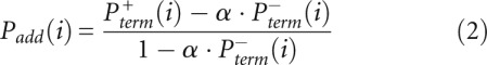
The Gaussian Peak Fitting algorithm performs whole-signal Gaussian integration for all peaks in the (+) and (−) reagent signals, fitting each peak with a Gaussian function individually optimized for position, height, and width. The area of each peak is correlated with the primer termination probability, P_term, of the corresponding nucleotide in the RNA sequence. The Scaling operation determines the magnitude of the scaling parameter α (Eq. 11). Normalization computes the probability of adduct formation, P_add, for each nucleotide using Equation 2. Although P_add is a true measure of the reactivity of a particular nucleotide, it is normalized using model-free statistics to a scale spanning 0 to ∼2, where zero indicates no reactivity and 1.0 is the average intensity for highly reactive RNA positions. Nucleotides with normalized SHAPE reactivities 0–0.4, 0.4–0.85, and >0.85 correspond to unreactive, moderately reactive, and highly reactive positions, respectively.

Output

The final output of QuShape is a tab-delimited text file. This file contains integrated (+) and (−) reagent peak areas and their normalized SHAPE reactivities. The final SHAPE reactivity plot is also displayed in a graphic window (Fig. 3D).

QuShape performance

When run in the default automatic mode, QuShape completes all data analysis steps involved in a typical SHAPE experiment in ∼10 min (precise time varies depending on RNA length and computer used). Visual inspection and any necessary manual alignment correction can extend the analysis time by 10–15 min. In contrast, the same analysis for a long RNA using ShapeFinder would require a motivated and trained user ∼2 h. The SHAPE reactivity values computed by QuShape are highly correlated with values obtained on the same raw data using ShapeFinder. For example, SHAPE analysis of a 403-nt region of the central domain of the Escherichia coli 16S rRNA yielded a correlation coefficient, r, of 0.98 (Fig. 4).

FIGURE 4.

Comparison of SHAPE reactivities measured at single-nucleotide resolution for a 403-nt region of the E. coli 16S rRNA using ShapeFinder and QuShape software. (A) QuShape and ShapeFinder reactivity estimates plotted as a function of nucleotide position in the RNA. (B) Correlation between QuShape and ShapeFinder per-nucleotide reactivity estimates. Pearson's r is shown.

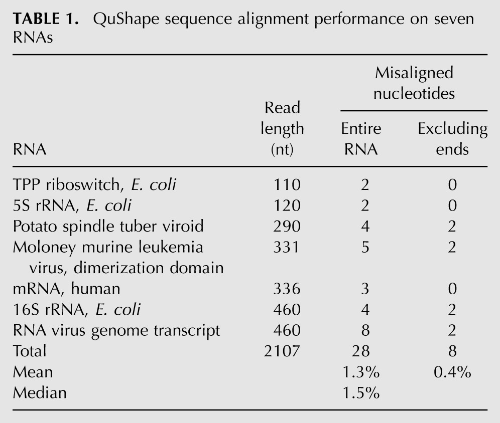
To evaluate QuShape, seven users each ran the program on a different type of RNA with which he or she was familiar. Except for the Sequence Alignment operation, the performance of all analytical steps was completely satisfactory and required no manual intervention. A total of 2107 nt were analyzed for both small (110 and 120 nt) and large (290 to 460 nt) RNA regions (Table 1). Each user attempted to obtain quantitative reactivity information from the longest readable region in their RNA. The Sequence Alignment procedure misaligned or misidentified 28 of the 2107 peaks, corresponding to an overall misalignment rate of 1.3% and a median misalignment rate of 1.5%. The majority of misaligned peaks were located in the first and the last 20 nt of the RNA sequence. If the noisy terminal regions (first and last 20 nt of each trace) were excluded, the misassignment error rate was 0.4% (Table 1). All errors were readily corrected using the graphic user interface tools to add or delete a peak, change a base label, or change a link between corresponding peaks in different traces. Critically, virtually all misassignments corresponded to ±1-nt shifts at a single nucleotide such that alignment errors are local. These errors, even if left uncorrected, have relatively small impact on interpretation of chemical probing information.

TABLE 1.

QuShape sequence alignment performance on seven RNAs

Reference-based analysis

In a significant efficiency advance, QuShape allows the results of a previous analysis to serve as a reference for subsequent analyses on the same RNA. The FAST software (Pang et al. 2011) includes a similar feature. In QuShape, all parameters can be saved as a “reference” experiment such that subsequent analyses of the same RNA are processed fully automatically. RNA sequence alignment is the most data quality sensitive and algorithmically challenging step in any pipeline for interpreting chemical probing experiments by capillary electrophoresis. Although QuShape appears to be the most accurate processing software currently available, misalignments were observed. With QuShape, this manual correction is performed once for a given RNA. For all subsequent SHAPE experiments, the saved “reference” alignment is used, producing essentially errorless quantitative results (Fig. 5). Reference-based analysis makes it straightforward to evaluate the same RNA under multiple conditions or to quantify time-resolved experiments with many time points, for example.

FIGURE 5.

QuShape analysis by reference. An automated sequence alignment of TPP riboswitch RNA traces is shown. Sequence alignment was achieved by aligning experimental traces [(+) and (−) reagent] with a sequence trace from an independent experiment. The ddNTP and (+) and (−) reagent traces from the reference experiment are drawn in light colors. Because these experiments were performed under different conditions, many nucleotides exhibit distinctly different fluorescence intensities in their (+) reagent traces; nevertheless, QuShape completed the reference-based analysis of this experiment in <1 min without error.

DISCUSSION

QuShape was developed to address the practical challenges in investigating nucleic acid structure and ligand interactions using chemical probing technologies, as resolved by automated capillary electrophoresis. The foremost requirements are accuracy and speed. There is often a trade-off between automation of a data processing pipeline and accuracy, and serious errors can be introduced by algorithms that do not fully account for subtleties in the structure of chemical probing data (see Leonard et al. 2012). In developing QuShape, we sought to maximize the quantitative accuracy of extracting reactivity information from CE electropherograms by optimizing and customizing each step and to minimize processing time by automating as much of the process as possible while maintaining accuracy and the ability of users to intervene.

Algorithmic innovations in QuShape—described in detail in the Materials and Methods—include new approaches for signal decay correction, signal alignment, base calling, sequence alignment, and scaling. The signal decay correction procedure estimates probabilities of termination for the primer extension reaction using an algorithm outlined previously (Aviran et al. 2011b). Our algorithm differs in its improved quantitative and experimentally informed treatment of the missing information at the end of the time-elution signal. Signal alignment has been improved significantly using a dynamic programming algorithm that incorporates a new measure of peak similarity and control of the sequence gap penalty (Karabiber et al. 2011). The newly developed base-calling algorithm avoids peak misclassification errors that primarily reflect large peaks that do not correspond to authentic sequencing peaks. The new sequence alignment procedure, based on the Smith–Waterman algorithm, is made much more effective by using a cost matrix that reflects the degree of uncertainty in peak labels and by controlling peak spacing. Finally, the new algorithm for scaling the (−) reagent signal relative to the (+) reagent signal is highly accurate and fully automated.

QuShape runs under Windows, MacOS/X, and Linux and uses open source software. No additional software is required to perform a complete analysis of raw capillary electrophoresis data. Most users will find that QuShape performs well when run in an automatic mode by executing the default series of analytical procedures (Fig. 2B); it also contains alternative algorithmic procedures that may be useful for specific analysis challenges. The graphic user interface makes it straightforward to read data, visually monitor the quality of intermediate data processing steps, and, if necessary, execute alternative procedures. Manual correction of (usually very small) sequence alignment errors needs to be completed only once for a given RNA. This alignment can then be used efficiently in all the subsequent experiments on the same RNA using the analysis-by-reference option, significantly reducing total analysis time.

We recommend the two-capillary experimental approach (Fig. 2A) rather than a single-capillary protocol or alignment procedures that make use of an additional marker or ladder channel. Two-capillary resolution nicely balances the goals of efficient experimentation with accurate sequence alignment. However, QuShape can be used to analyze data obtained with either single- or two-capillary approaches. QuShape can be used to analyze capillary electrophoresis data from any class of nucleic acid reactivity probing experiment including those that use conventional chemical modification agents or hydroxyl radicals to map structure and solvent accessibility. In sum, QuShape is a comprehensive, platform-independent, user-friendly, and complete software package that enables efficient, reliable, highly automated, and accurate analysis of high-throughput capillary electrophoresis–detected nucleic acid chemical-probing experiments.

MATERIALS AND METHODS

Software implementation, data acquisition, and file formats

All tools and methods were implemented using version 2.6 of the Python programming language (http://www.python.org/). PyQt (http://www.riverbankcomputing.co.uk/pyqt/index.php) was used for designing the user interface and runs on all platforms supported by Qt including Windows, MacOS/X, and Linux. NumPy and SciPy are the fundamental packages needed for scientific computing in Python (http://numpy.scipy.org/) and were used to manipulate data and arrays. Matplotlib (http://matplotlib.sourceforge.net/), a Python 2D plotting library, is used to produce quality figures in a variety of hard-copy formats and interactive environments across platforms. All packages are open source software. QuShape can read ABI data formats .fsa and .ab1 as well as tab-delimited text files, which facilitates analysis of electropherograms from older instruments and those using legacy data formats. QuShape also reads the ShapeFinder report file. QuShape can be used to analyze data obtained from a single-capillary (three or four color) experiment by selecting the (+) and (−) reactions from the single-capillary data file and specifying channel numbers appropriately when creating the QuShape project (the sequencing trace will be the same for each channel). When acquiring data, the instrument should be set to “Fragment Analysis” and “No Normalization” modes and to the appropriate dye set (G5 or F for ABI instruments). If normalization cannot be disabled, set the size-calling analysis range to the first point (0 to 1) of the trace. We have used ABI 3130 and 3500 instruments with either 36- or 50-cm capillaries filled with the ABI POP-7 polymer matrix; other instruments also work well. Injection times are generally 8–10 sec but can be set longer to resolve low-concentration samples.

Two-capillary protocol

The original SHAPE experiment used four different fluorescently labeled primers for the (+) and (−) reagent experiments and the two ddNTP sequencing reactions; all reactions were then resolved in a single capillary (Vasa et al. 2008). In QuShape, we recommend an experimental and signal processing pipeline that requires only two fluorescent labels. The four samples are resolved in two capillaries: the (+) reagent reaction and one sequencing reaction in one capillary and the (−) reagent reaction and an identical sequencing reaction in a second capillary (Fig. 2). This two-capillary approach uses only two dyes, which are chosen to impart similar mobility shifts to their respective cDNA fragments and simultaneously have sufficiently different fluorescent emission spectra to facilitate straightforward spectral deconvolution. We typically use VIC and NED (Applied Biosystems) or 5-FAM and 6-JOE (Anaspec). Other two-dye systems can also be used. QuShape supports mobility shifts for the following dyes: 5-FAM, 6-FAM, TET, HEX, 6-JOE, NED, VIC, TAM, and ROX. To reduce mobility shift errors, both dyes should be either fluorescein (5-FAM, 6-FAM, TET, HEX, 6-JOE, NED, VIC) or rhodamine (TAM, ROX) derivatives. This approach has advantages over both single-capillary and align-to-marker methods: (1) Use of only two dyes reduces primer preparation requirements; (2) errors in signal alignment resulting from differences in dye-imparted mobility shifts are significantly reduced; (3) use of the sequencing lane for a marker allows the data to be more precisely aligned with a sequence; and (4) use of the same sequence marker makes aligning multiple data sets more reliable.

SHAPE data

SHAPE experiments were performed as outlined previously (Wilkinson et al. 2006; McGinnis et al. 2009); final samples contained 0.5–5 pmol of fluorescently labeled cDNA in 10-μL deionized formamide. Experiments with minor RNA-specific variations have been reported for the TPP riboswitch (Steen et al. 2012), a retroviral genome signaling domain (Gherghe et al. 2010; Grohman et al. 2011), ribosomal RNAs (Deigan et al. 2009; McGinnis et al. 2012), and long viral RNAs (Wilkinson et al. 2008; Watts et al. 2009; Gherghe et al. 2010). The key new feature is that all experiments are now resolved in two capillaries. For the VIC/NED and 5-FAM/6-JOE pairs, the first dye was used to perform primer extension for the (+) and (−) reactions, and the second dye was used for the single sequencing reaction. The sequencing reaction can be performed at a large scale (typically 20–50 reactions), aliquoted, stored in the dark at −20°C, and used as needed. Sequencing reactions can be performed using either RNA (Wilkinson et al. 2006; McGinnis et al. 2009) or DNA (Watts et al. 2009) templates.

Data-processing innovations

Signal decay correction

A characteristic feature of fluorescent signals in a SHAPE (or any chemical probing) experiment electropherogram is that intensity gradually declines as a function of the elution time (Fig. 6A, top). This gradual decline is due to two phenomena: (1) The reverse transcriptase enzyme is not perfectly processive, and (2) a subset of RNAs contains multiple adducts or other features that prevent reverse transcription, and the enzyme stops at the lesion nearest the 3′ end. The population of extending primers thus gradually decreases with RNA length due to termination at each successive nucleotide. If the probability of primer termination were the same for each nucleotide, then the signal intensity I would decline as a function of nucleotide position t according to:

where I₀ is the starting intensity and p is the probability of terminating extension at any given nucleotide (Vasa et al. 2008). This model serves as the basis for the signal decay correction algorithms in ShapeFinder and FAST (Pang et al. 2011). In fact, however, primer termination probabilities vary across nucleotides.

FIGURE 6.

Illustration of key signal processing steps. (A) Signal decay correction. (Top) An unprocessed full-length electropherogram corresponding to the (+) reagent reaction. (Bottom) The same trace corrected using the algorithm based on Equations 6 and 7. (B) Base calling. Alignment and superimposition of a (−) reagent signal and a γ-scaled (Eq. 8) sequencing signal, both obtained in the same (−) reagent capillary. Aligned peaks in the two signals correspond to individual nucleotides in the RNA sequence. The nucleotide base identity of each peak is indicated by a letter (A, C, G, U). The sequenced base in this experiment was guanosine (G). Note that the G peaks vary in their heights as do the peaks produced by non-G nucleotides, such that it is impossible to unambiguously distinguish G and non-G peaks solely by height. In contrast, the difference in heights of the same peak in the (−) reagent and sequencing signals reliably separates G from non-G peaks. (C) Scaling of (+) reagent and (−) reagent signals. Points correspond to (−) reagent versus (+) reagent termination probabilities, P_term(i), for 353 nucleotides in the E. coli 16S rRNA obtained in a SHAPE experiment. Nucleotides with the lowest 20% (+) reagent termination probability are black; all other nucleotides are blue. The least-squares linear approximation of the black data points is shown as a red line and yields the scaling parameter α (used in Eq. 2).

To develop a more accurate signal decay correction algorithm, we note that measured fluorescence intensities in an electropherogram trace reflect both P_term and the size of the extending primer population:

where I(i) is the signal intensity at the i-th nucleotide along the elution time axis, is the probability of primer termination at nucleotide i, and N(i) is the size of the primer population reaching nucleotide i. Since

P_term equals:

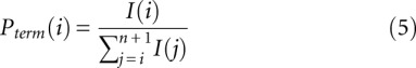where n is the total number of nucleotides, and n + 1 indicates the signal produced by the primers that extended the full length of the RNA. An alternative theoretical derivation of Equation 5 has been described (Aviran et al. 2011a,b), but our much simpler framework (Eqs. 4 and 5) yields the identical analytical expression.

The critical, and thus far incompletely resolved, practical constraint in using Equation 5 reflects that the signal can be very strong at the end of capillary electropherogram due to cDNAs that extend the full length of the RNA, often causing detector saturation (Fig. 6A, emphasized with asterisks). Signal intensities associated with the end of the RNA are therefore not measured, which introduces error in estimating .

A heuristic solution to this loss of information reflects the expectation that, on average, probabilities of termination of primer extension for the first and second halves of the RNA are the same (Vasa et al. 2008; Pang et al. 2011). Thus can be computed as:

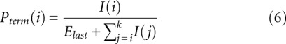where k is the last accurately measured nucleotide and E_last is the expected sum of intensities after the k-th nucleotide [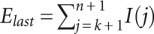]. The value of E_last is chosen to minimize the difference between the first and second halves of the trace:

A conceptually similar heuristic solution is used in the FAST program (Pang et al. 2011). In extensive testing, signal decay correction based on Equations 6 and 7 produces robust results (Fig. 6A, bottom).

Alignment of signal peaks with RNA sequence

The electropherogram traces corresponding to the (+) and (−) reactions exhibit a series of roughly evenly spaced bell-shaped peaks of varying heights (Fig. 3). To assign each peak to its corresponding RNA position, the dideoxy nucleotide (ddNTP) sequencing traces are first matched against the known RNA nucleotide sequence, thus establishing the nucleotide identity of peaks in the sequencing traces, and then the annotated sequencing peaks are aligned with peaks in the (+) reagent and (−) reagent traces.

To assign each peak in a sequencing trace to its corresponding RNA position, it is first necessary to determine the base identity of each peak. Sequencing traces contain two classes of peaks: “specific” peaks produced by ddNTP-paired nucleotides and “nonspecific” or background peaks corresponding to nucleotides of the other three bases. The identity of these peaks is underdetermined. Generally, but not always, specific sequencing peaks are larger than background peaks, and this difference can be used to distinguish them via a classification threshold. The misclassification frequency can be reduced by matching peaks between the sequencing signal and the corresponding peaks in the (−) reagent signal, since some of the within-class variability of peak sizes is common to both signals. To identify the specific peaks using this approach, peaks in the sequencing signal are first linked with their counterparts in the (−) reagent signal. The sequencing signal is then scaled by a gain parameter, γ, to make it comparable to the (−) reagent signal. The magnitude of γ is determined by minimizing the difference Δ:

where S₅₀ is the set of all the peaks whose sizes in the sequencing signal are below the median size of the peaks in the sequencing signal, and I^s(i) and I⁻(i) are the sizes of the i-th peaks in the sequencing and (−) reagent signals, respectively. Finally, after scaling the sequencing peaks by γ, peaks with the size ratio 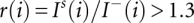are classified as specific sequencing peaks and defined as the base complementary to the ddNTP used; all the other peaks are classified as nonspecific and labeled N (Fig. 6B).

The next step is to align peaks in the sequencing signal with the known RNA sequence. Several factors complicate this task. Excessive and undifferentiated fluorescence at the start and the end of the electropherogram trace obscures peaks that correspond to nucleotides at either end of the studied RNA (Fig. 6A). Thus, the usable segment of the sequencing trace and its exact placement along the RNA length must be determined. In broad terms, this sequence alignment or matching step can be accomplished by matching the sequenced peaks (those with known base identity) with the same-base nucleotides in the RNA sequence. In practice, this is the most challenging step in automated processing of nucleic acid probing data: Some peaks are misclassified, some peaks are missed, and some identified peaks are extraneous and should not be counted as a nucleotide. All software developed to date to perform this step produces numerous errors that either have to be corrected manually or, if left uncorrected, lead to significant reactivity misassignments.

To achieve a significant increase in the accuracy of sequence alignment, we made use of the Smith–Waterman local alignment algorithm (Smith and Waterman 1981). In the Smith–Waterman algorithm, a query sequence is matched and scored against a longer reference sequence to derive similarity scores for all possible subsequences of the reference sequence. Smith–Waterman utilizes a scoring matrix to assign the score to each putative nucleotide pair based on a predefined cost matrix and a scoring rule. The optimal subsequence is extracted using a traceback matrix.

QuShape tailors the alignment cost matrix to the specific characteristics of chemical probing data. In the cost matrix, we incorporated a confidence term in our designation of a particular peak as being a specific peak (NT) or a nonspecific peak (N) using its size ratio, r(i):

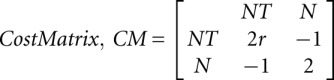The scoring and traceback matrices are filled using the following scoring rule:

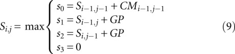where i and j are the indices of the nucleotides in the RNA sequence and peaks in the sequencing signal, respectively; CM_i−1,j−1 is the cost matrix value for the (i − 1), (j − 1) nucleotide-peak pair; and GP is the gap penalty. The maxima of the values {s₀, s₁, s₂, s₃} are used to fill the score and traceback matrices.

Since peaks are spaced fairly evenly in the sequencing trace, missed peaks or mistakenly recognized peaks can often be detected automatically before application of the Smith–Waterman sequence alignment. Because of this peak spacing control, more than one consecutive gap in the traceback reconstruction of the best alignment is rare, and, therefore, consecutive gaps are not allowed in the reconstruction phase. Gaps identified by the Smith–Waterman procedure are automatically removed by adding or deleting peaks. If there is a gap in the reconstructed sequencing list, a peak is inserted at the largest space between peaks. If there is a gap in the reconstructed RNA list, the smallest-width peak is deleted from the reconstructed sequencing list between the matched sequenced peaks. With these enhancements to the original Smith–Waterman algorithm, we routinely obtained RNA sequence alignments that were ≥98% correct. Furthermore, misalignments, when they occurred, were local (typically ±1 nt) in contrast to prior automatic alignment approaches that yield offsets that extend over many nucleotides. These local misalignments are easily corrected manually in QuShape.

Scaling

Because the (+) and (−) reagent primer extension reactions are performed separately and not necessarily under fully identical conditions, the probability of spontaneous primer termination at any given nucleotide [P_spont(i), Eq. 1] cannot be assumed to be the same in both the (+) reagent and (−) reagent conditions. To compute the SHAPE reactivity of any given nucleotide [P_add(i); Eqs. 1 and 2], it is necessary to determine the scaling of P_spont in the (−) reagent condition relative to P_spont in the (+) reagent condition (Eq. 2, parameter α). A physically realistic model is that the nucleotides that produced the smallest peaks in the (+) reagent signal had approximately zero probability of forming an adduct; therefore, primer termination at these nucleotides was due solely to spontaneous causes such that:

In ShapeFinder, this scaling was performed manually by visually matching the smallest 5%–10% of peaks in the (+) and (−) reagent signals. To automate this step, we identify a set, S₂₀, of the 20% of nucleotides with the smallest , measured according to Equations 6 and 7. The magnitude of the scaling parameter α is determined by minimizing the difference E between termination probabilities of these nucleotides in the (+) reagent and (−) reagent conditions:

as illustrated in Figure 6C.

Availability

QuShape is freely downloadable from http://www.chem.unc.edu/rna/qushape under the GNU General Public License, version 3. QuShape also has an extensive help guide and new user tutorial.

REFERENCES

- Aviran S, Trapnell C, Lucks JB, Mortimer SA, Luo S, Schroth GP, Doudna JA, Arkin AP, Pachter L 2011a. Modeling and automation of sequencing-based characterization of RNA structure. Proc Natl Acad Sci 108: 11069–11074 [DOI] [PMC free article] [PubMed] [Google Scholar]
- Aviran S, Lucks JB, Pachter L 2011b. RNA structure characterization from chemical mapping experiments. Communication, Control, and Computing (Allerton), 49th Annual Allerton Conference, 28–30 September 2011, pp. 1743–1750. http://math.berkeley.edu/∼saviran/Aviran_Allerton_2011.pdf [Google Scholar]
- Deigan KE, Li TW, Mathews DH, Weeks KM 2009. Accurate SHAPE-directed RNA structure prediction. Proc Natl Acad Sci 106: 97–102 [DOI] [PMC free article] [PubMed] [Google Scholar]
- Gherghe CM, Shajani Z, Wilkinson KA, Varani G, Weeks KM 2008. Strong correlation between SHAPE chemistry and the generalized NMR order parameter (S2) in RNA. J Am Chem Soc 130: 12244–12245 [DOI] [PMC free article] [PubMed] [Google Scholar]
- Gherghe C, Lombo T, Leonard CW, Datta SAK, Bess JW, Gorelick RJ, Rein A, Weeks KM 2010. Definition of a high-affinity Gag recognition structure mediating packaging of a retroviral RNA genome. Proc Natl Acad Sci 107: 19248–19253 [DOI] [PMC free article] [PubMed] [Google Scholar]
- Grohman JK, Kottegoda S, Gorelick RJ, Allbritton NL, Weeks KM 2011. Femtomole SHAPE reveals regulatory structures in the authentic XMRV RNA genome. J Am Chem Soc 133: 20326–20334 [DOI] [PMC free article] [PubMed] [Google Scholar]
- Karabiber F, Weeks KM, Favorov OV 2011. Automated peak alignment for nucleic acid capillary electrophoresis data by dynamic programming. BCB'11 Proceedings of the 2nd ACM Conference on Bioinformatics, Computational Biology and Biomedicine, ACM New York, NY, pp. 544–546 [Google Scholar]
- Leonard CW, Hajdin CE, Karabiber F, Mathews DH, Favorov OV, Dokholyan NV, Weeks KM 2012. Principles for understanding the accuracy of SHAPE-directed RNA structure modeling. Biochemistry doi: 10.1021/bi300755u [DOI] [PMC free article] [PubMed] [Google Scholar]
- Lucks JB, Mortimer SA, Trapnell C, Luo S, Aviran S, Schroth GP, Pachter L, Doudna JA, Arkin AP 2011. Multiplexed RNA structure characterization with selective 2′-hydroxyl acylation analyzed by primer extension sequencing (SHAPE-seq). Proc Natl Acad Sci 108: 11063–11068 [DOI] [PMC free article] [PubMed] [Google Scholar]
- McGinnis JL, Duncan CDS, Weeks KM 2009. High-throughput SHAPE and hydroxyl radical analysis of RNA structure and ribonucleoprotein assembly. Methods Enzymol 468: 67–89 [DOI] [PMC free article] [PubMed] [Google Scholar]
- McGinnis JL, Dunkle JA, Cate JH, Weeks KM 2012. The mechanisms of RNA SHAPE chemistry. J Am Chem Soc 134: 6617–6624 [DOI] [PMC free article] [PubMed] [Google Scholar]
- Merino EJ, Wilkinson KA, Coughlan JL, Weeks KM 2005. RNA structure analysis at single nucleotide resolution by selective 2′-hydroxyl acylation and primer extension (SHAPE). J Am Chem Soc 127: 4223–4231 [DOI] [PubMed] [Google Scholar]
- Mitra S, Shcherbakova IV, Altman RB, Brenowitz M, Laederach A 2008. High-throughput single-nucleotide structural mapping by capillary automated footprinting analysis. Nucleic Acids Res 36: e63 doi: 10.1093/nar/gkn210 [DOI] [PMC free article] [PubMed] [Google Scholar]
- Nielsen PE 1990. Chemical and photochemical probing of DNA complexes. J Mol Recognit 3: 1–25 [DOI] [PubMed] [Google Scholar]
- Pang PS, Elazar M, Pham EA, Glenn JS 2011. Simplified RNA secondary structure mapping by automation of SHAPE analysis. Nucleic Acids Res 39: e151 doi: 10.1093/nar/gkr773 [DOI] [PMC free article] [PubMed] [Google Scholar]
- Ritz J, Martin JS, Laederach A 2012. Evaluating our ability to predict the structural disruption of RNA by SNPs. BMC Genomics (Suppl. 4) 13: S6 doi: 10.1186/1471-2164-13-S4-S6 [DOI] [PMC free article] [PubMed] [Google Scholar]
- Smith TF, Waterman MS 1981. Identification of common molecular subsequences. J Mol Biol 147: 195–197 [DOI] [PubMed] [Google Scholar]
- Steen K-A, Rice GM, Weeks KM 2012. Fingerprinting non-canonical and tertiary RNA structures by differential SHAPE reactivity. J Am Chem Soc 134: 13160–13163 [DOI] [PMC free article] [PubMed] [Google Scholar]
- Vasa SM, Guex N, Wilkinson KA, Weeks KM, Giddings MC 2008. ShapeFinder: A software system for high-throughput quantitative analysis of nucleic acid reactivity information resolved by capillary electrophoresis. RNA 14: 1979–1990 [DOI] [PMC free article] [PubMed] [Google Scholar]
- Watts JM, Dang KK, Gorelick RJ, Leonard CW, Bess JW Jr, Swanstrom R, Burch CL, Weeks KM 2009. Architecture and secondary structure of an entire HIV-1 RNA genome. Nature 460: 711–716 [DOI] [PMC free article] [PubMed] [Google Scholar]
- Weeks KM 2010. Advances in RNA structure analysis by chemical probing. Curr Opin Struct Biol 20: 295–304 [DOI] [PMC free article] [PubMed] [Google Scholar]
- Weeks KM 2011. RNA structure probing dash seq. Proc Natl Acad Sci 108: 10933–10934 [DOI] [PMC free article] [PubMed] [Google Scholar]
- Wilkinson KA, Merino EJ, Weeks KM 2006. Selective 2′-hydroxyl acylation analyzed by primer extension (SHAPE): Quantitative RNA structure analysis at single nucleotide resolution. Nat Protoc 1: 1610–1616 [DOI] [PubMed] [Google Scholar]
- Wilkinson KA, Gorelick RJ, Vasa SM, Guex N, Rein A, Mathews DH, Giddings MC, Weeks KM 2008. High-throughput SHAPE analysis reveals structures in HIV-1 genomic RNA strongly conserved across distinct biological states. PLoS Biol 6: e96 doi: 10.1371/journal.pbio.0060096 [DOI] [PMC free article] [PubMed] [Google Scholar]
- Wilkinson KA, Vasa SM, Deigan KE, Mortimer SA, Giddings MC, Weeks KM 2009. Influence of nucleotide identity on ribose 2′-hydroxyl reactivity in RNA. RNA 15: 1314–1321 [DOI] [PMC free article] [PubMed] [Google Scholar]
- Yoon S, Kim J, Hum J, Kim H, Park S, Kladwang W, Das R 2011. HiTRACE: High-throughput robust analysis for capillary electrophoresis. Bioinformatics 27: 1798–1805 [DOI] [PubMed] [Google Scholar]