Rank reversal in indirect comparisons

Abstract

Objective

To describe rank reversal as a source of inconsistent interpretation intrinsic to indirect comparison (Bucher et al., 1997) of treatments and to propose best practice.

Methods

We prove our main points with intuition, examples, graphs, and mathematical proofs. We also provide software and discuss implications for research and policy.

Results

When comparing treatments by indirect means and sorting them by effect size, three common measures of comparison (risk ratio, risk difference, and odds ratio) may lead to vastly different rankings.

Conclusions

The choice of risk measure matters when making indirect comparisons of treatments. The choice should depend primarily on the study design and conceptual framework for that study.

Introduction

When a direct comparison of two or more treatments within the same study is not possible, researchers must instead make indirect comparisons of those treatments across different trials. Bucher and colleagues [1] first showed how to conduct an indirect comparison meta-analysis. Under the assumption that the relative efficacy of the treatments are consistent for patients in the different trials [2,3], Bucher and colleagues [1] show that the log odds of the adjusted indirect comparison of two treatments (each compared to a placebo or common control treatment) is a simple function—the difference in the log odds ratio of each treatment compared to its control. Their basic method has proved quite influential. While others have expanded upon it [3,4,5], the basic model has been used in numerous meta-analyses.

Although Bucher and colleagues present their model using odds ratios, they also assert that the “method could be equally applied to estimates of relative risk” (Bucher et al., 1997, p. 684). Song and colleagues (2000, p. 489) state that Bucher’s method of adjusted indirect comparison “may also be used when the relative efficacy is measured by risk ratio or by risk difference.” Indeed, there are a few studies that have modified the formulas appropriately and used either the risk ratio or the risk difference instead of the more common odds ratio (e.g., [6]).

The central point of this paper is that when indirectly comparing two or more treatments, the choice of how to express results may directly affect the conclusion. In other words, when sorting treatments by effect size (which we refer to as ranking), the choice between risk ratio, risk difference, and odds ratio matters. We describe these three measures and show when indirect comparisons using any of the measures will be different from the others. We illustrate our results with intuition, examples, graphs, and mathematical proofs. We are unaware of previous description of this phenomenon, which we call rank reversal.

We explain our main points in the context of an indirect comparison meta-analysis, whereby two treatments (let’s call them A and B) are each compared to a control (called C) in separate studies. The goal is to use the information in these two separate studies to indirectly compare treatments A and B, and thereby rank their effectiveness. For example, compared to a placebo, is the desirable outcome more likely when a patient takes drug A rather than drug B? The answer to this question is important for both practice and policy. As we explain, answering this question is not always straightforward. When compared to their respective placebos, drug A may be preferred to drug B when measured by a risk ratio, but drug B may be preferred to drug A when measured by an odds ratio, even though both odds ratio and risk ratio are measures of relative effectiveness.

We prove that rankings are not always consistent across these risk measures, describe under what circumstances the rankings are the same or different, explain how uncertainty affects the main results, introduce software that can help identify problems, discuss implications, and recommend best practice for research and policy. When the study design is such that the results could be expressed in terms of either risk ratios or odds ratios, the burden is on the researcher to specify a conceptual framework to make that choice.

Methods

Consider pairs of probabilities (R₀, R₁), with R₀ referring to the baseline (control) risk and R₁ to the risk if treated. These risks are defined as probabilities of an event during a specified period of time [7], and so are bounded by zero and one. For any pair of probabilities (R₀, R₁) we can define the risk ratio, risk difference, and odds ratio with R₀ as the reference.

$$RR=\frac{R_1}{R_0}$$ (1)

$$RD=R_1-R_0$$ (2)

$$OR=\frac{\frac{R_1}{(1-R_1)}}{\frac{R_0}{(1-R_0)}}$$ (3)

We state two proofs, and direct the reader to the Appendix in Supplemental Materials at: XXX for the details of those proofs. First, within a single study, where baseline risk is the same, treatment alternatives will have the same ranking regardless of the risk measure used. In other words, all three risk measures are strictly monotonic in changes in risk to the treatment group (R₁). Second, if both R₀ and R₁ are allowed to change then there can be rank reversal. That is, two treatment options A and B and their respective control treatments, represented by the pairs of points $(R_0^A,R_1^A)$ and $(R_0^B,R_1^B)$, may be ranked differently by the risk ratio, risk difference, and odds ratio. The total derivative of each measure (with respect to both R₀ and R₁) can have different signs, indicating rank reversal. For details, see the Appendix in Supplemental Materials at: XXX.

Graphs

It is easy to show rank reversal with graphs (see [8] for similar graphs). Each pair of probabilities can be plotted on a unit square graph. If treatment and baseline risks are the same, i.e., R₁ = R₀, then the point falls along the 45-degree line. If the treatment risk is higher than the baseline risk, then the point lies to the northwest of the 45-degree line.

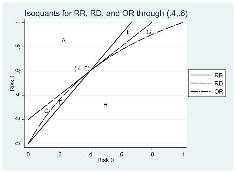
For any point (R₀, R₁) on the graph, isoquants show all other points with the same value of the risk ratio, risk difference, or odds ratio (see Figure 1 for an example with (R₀, R₁)=(0.4,0.6)). Isoquants are a set of points (lines) that all have the same value of a quantity, such as the RR, RD, or OR. By definition, all three isoquants in this example must pass through the point (0.4, 0.6). The risk ratio isoquant is a ray from the origin with slope of 1.5 = 0.6/0.4. The risk difference isoquant is parallel to the 45-degree line, with the intercept on the y-axis equal to 0.2 = 0.6–0.4. The odds ratio isoquant is an arc connecting the origin to the point (1, 1) such that the odds ratio along the arc is always 2.25 = [0.6 / (1–0.6)]/[0.4 / (1–0.4)].

Figure 1.

Isoquants for the point (.4, .6).

The intuition of the first proof is shown graphically by moving due north of (0.4, 0.6) in Figure 1. All those northerly points lie on isoquants representing RR values greater than 1.5, RD values greater than 0.2, and OR values greater than 2.25. Moving due north is the graphical equivalent of taking a derivative with respect to R₁ (positive change in R₁, holding R₀ constant). Similarly, moving due south of the point falls below all three isoquants (negative change in R₁ only). That intuition holds for any pair of risks, including those below the 45-degree line or not on the negative 45-degree line. For any fixed baseline risk R₀, the rankings of any two treatments will be the same for RR, RD, and OR.

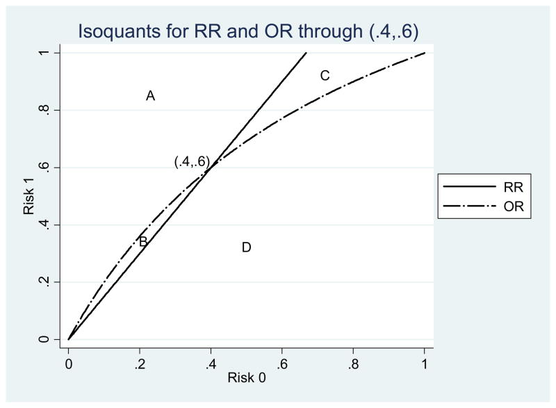
The situation changes when comparing points that do not share the same baseline risk R₀. To make our point simpler, we have redrawn Figure 1 without the RD isoquants, to focus only on RR and OR (see Figure 2). We can compare any point to (0.4, 0.6) and ask: Is one risk ratio higher than the other? Do the risk ratios and odds ratios have the same ranking? If the other point lies to the northwest of (0.4, 0.6) in the area marked A, then it will have higher values of both RR and OR. If it lies to the southeast (large area marked D) then it will have lower values of both RR and OR. In these cases, both RR and OR rank these points the same; there is no rank reversal.

Figure 2.

Isoquants for the point (.4, .6).

The interesting cases lie to the southwest and to the northeast in the areas marked B and C. For example, take the point (0.6, 0.8) in area C. This point has a lower RR than (0.4, 0.6) (RR = 1.33 instead of 1.5); as such, it lies below the RR isoquant. But it has a higher OR than the point (0.4, 0.6) and lies above the OR isoquant. Therefore, (0.6, 0.8) has a different ranking compared to (0.4, 0.6) when using RR than when using OR.

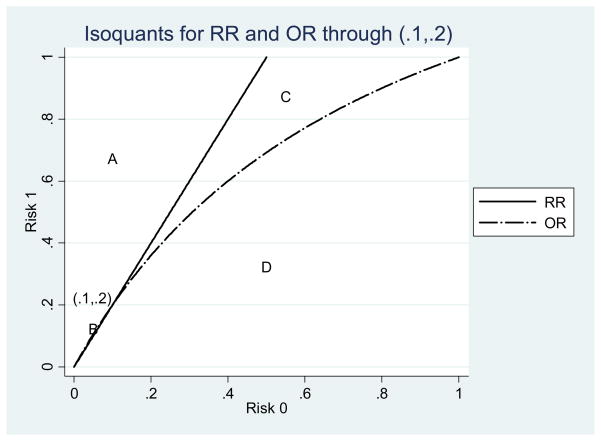
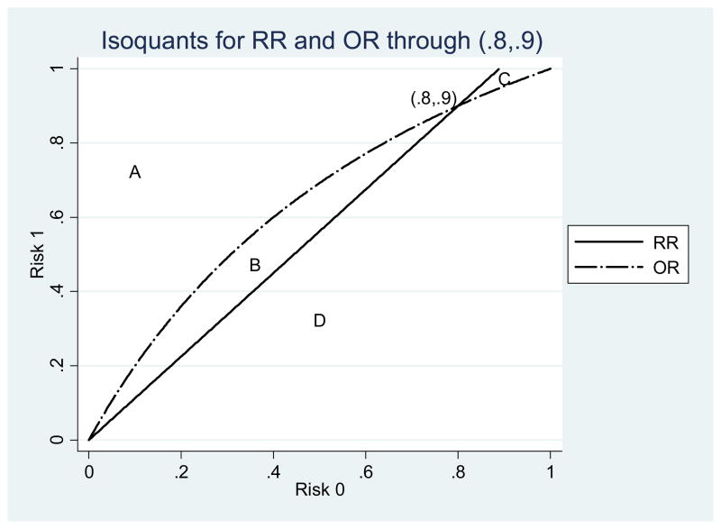
We show two other examples, again focusing on just RR and OR. Both examples lie along the same OR isoquant, so only the RR is changing. One has a tiny area B and a relatively large area C (see Fig. 3). The other is the opposite, with area B being much larger than area C (see Fig. 4). These examples show that location on the graph affects the probability that other points in the vicinity will have rank reversal problems. When both risks are small the chance that the OR of another point nearby exceeds the RR is almost zero.

Figure 3.

Isoquants for the point (.1, .2).

Figure 4.

Isoquants for the point (.8, .9).

Finally, to bring RD back into the picture we return to Figure 1 which has all three isoquants. In this figure we see that there are eight different regions, not four. In two of them (A and H) there are no rank reversals. The remaining areas (B through G) have one measure that disagrees with the other two measures about which point has a higher numerical value. For example, points in area E have a lower RR than (0.4, 0.6) but higher RD and OR. When given the same data for an indirect comparison or meta-analysis, researchers who report RR or OR could reach different conclusions about which treatment is preferred, given that the baseline risks are different. The areas B and F do not appear in Figure 1.

In summary, after drawing a point (R₀, R₁) on the graph and the corresponding three isoquants, then only the points entirely above all three isoquants or entirely below all three have the same ranking on all measures. While the area of the graph with the same ranking is always in the majority, in our experience reading the literature, studies that are compared to each other often lie broadly along the southwest to northeast corridor, making the choice of measure (RR, RD, or OR) important in the final comparison (e.g., [9]).

Uncertainty

Thus far we have assumed that the risks are known with certainty, as opposed to being estimated with error. In real clinical trials, however, risks are estimated with uncertainty (with confidence intervals or standard errors). This uncertainty does not change the basic conclusions of this paper, namely that different risk measures can lead to different rank ordering. However, with uncertainty the comparisons of risk become probabilistic instead of deterministic. That is, if one bootstrapped the rankings, taking draws of each risk from the estimated distribution of risks, and then computed the risk measures, the ranking may not always be the same.

Software

We have written Stata software that illustrates rank reversal for any baseline risk (R₀) and risk if treated (R₁). The program, called graphiso, takes as input any risk pair (R₀, R₁) and produces a graph with isoquants for each of the three risk measures (RR, RD and OR). In addition, the program calculates the areas for which each of the three risk measures generates a different ranking. The areas can only be interpreted as probabilities of rank reversal in the unlikely case of a uniform distribution of risk. This program file and a help file are available from the authors upon request.

As an example, our Stata program can recreate Figure 1 for (R₀, R₁)=(0.4, 0.6) and calculate areas with the command graphiso .4 .6. The program displays the following table of areas:

*********************RESULTS********************
Above RR, Above RD, Above OR 0.2933
Above RR, Above RD, Below OR 0.0000
Above RR, Below RD, Above OR 0.0239
Above RR, Below RD, Below OR 0.0161
Below RR, Above RD, Above OR 0.0267
Below RR, Above RD, Below OR 0.0000
Below RR, Below RD, Above OR 0.0239
Below RR, Below RD, Below OR 0.6161
Total area =           1
************************************************
************************************************
All same   0.9095
OR different 0.0239
RR different 0.0428
RD different 0.0239
************************************************

In this example, the two areas where all three measures agree on the ranking (areas A and G) together comprise 90 percent of the area of the unit square (see Fig. 1). Measuring risk using an odds ratio generates a ranking different from the other two measures in region G, which has an area of 0.0239. However, areas B and F do not exist for this risk pair—it is impossible for another point to have a lower OR than (0.4, 0.6) while simultaneously having a higher RR and RD.

Best Practice Recommendations

Our results lead to several recommendations for best practice when making indirect comparisons. First, given the conceptual framework and study design, decide which measure is most appropriate for the research. There is an extensive literature on the differences between RR, RD, and OR (for guidance, see textbooks by [7,10,11,12] and articles [13,14,15]). For some study designs, such as case-control studies, only the odds ratio is possible. Attention should also be paid to clarity of presentation of results [16,17,18,19,20,21,22]. As a default, we recommend using one of the risk measures instead of the odds ratio, unless there is a conceptual justification favoring the odds ratio. Second, for studies that have a study design that allows appropriate reporting of either risk ratios or odds ratios [23], show whether the different measures would lead to the same or different rankings. Either the result is robust across measures or the authors should acknowledge that other measures would lead to different conclusions and discuss this finding in light of the conceptual model.

Conclusions

The federal government is currently advocating head-to-head clinical trials, with several drugs being tested at once against the same placebo. This design both avoids the problem of comparing treatments to different placebos, and also will increase dramatically the number of indirect comparisons being conducted in clinical research. While the methods of Bucher and colleagues [1] will inform the analysis of these trials, the results of this study demonstrate the importance of the choice of risk measure when conducting indirect comparisons. This study has several important conclusions. First, we have two main mathematical results. The first is that if comparisons are made within the same study to the same control then the three measures will always have the same ranking. The more interesting result is that the choice of risk measure matters when making indirect comparisons of treatments with different baseline risks. This result holds regardless of whether or not there is uncertainty about the risks.

Our results have strong policy implications. Because researchers often choose a risk measure out of convenience or habit, policy decisions based on treatment ranking may be driven in part by these arbitrary decisions. Researchers need to confront the problem by showing whether the results are sensitive to choice of risk measure, and explain which measure is preferred for their study and why. This supports the importance of the explicit statement of a conceptual model and reference to that model in supporting the choice of measures.

This brings us to our third main conclusion: non-linear functions are challenging to understand. The prior debate in the literature between risk ratios and odds ratios has often focused on the magnitude of the effect [18,20,22]. The linear risk difference offers complementary and valuable information. Risk ratios and odds ratios do not differ in their sign (direction), only in their numerical magnitude and therefore in their interpretation. Here we show a new problem. When making indirect comparisons, risk ratios and odds ratios can lead to opposite conclusions regarding which option to favor. Non-linear functions, like risk ratios and odds ratios, emphasize different aspects of risk and have different properties; these differences are consequential.

References

- 1.Bucher HC, Guyatt GH, Griffith LE, Walter SD. The Results of Direct and Indirect Treatment Comparisons in Meta-Analysis of Randomized Controlled Trials. J Clin Epi. 1997;50:683–91. doi: 10.1016/s0895-4356(97)00049-8. [DOI] [PubMed] [Google Scholar]
- 2.Song F, Glenny A-M, Altman DG. Indirect Comparison in Evaluating Relative Efficacy Illustrated by Antimicrobial Prophylaxis in Colorectal Surgery. Controlled Clinical Trials. 2000;21:488–97. doi: 10.1016/s0197-2456(00)00055-6. [DOI] [PubMed] [Google Scholar]
- 3.Glenny AM, Altman DG, Song F, Sakarovitch C, et al. Indirect comparisons of competing interventions. Health Technol Assess. 2005;9:1–134. doi: 10.3310/hta9260. [DOI] [PubMed] [Google Scholar]
- 4.Song F, Altman DG, Glenny AM, Deeks JJ. Validity of indirect comparison for estimating efficacy of competing interventions: Empirical evidence from published meta-analyses. BMJ. 2003;326:472–5. doi: 10.1136/bmj.326.7387.472. [DOI] [PMC free article] [PubMed] [Google Scholar]
- 5.Eckermann S, Coory M, Willan AR. Indirect comparison: Relative risk fallacies and odds solution. J Clin Epidemiol. 2009;62:1031–36. doi: 10.1016/j.jclinepi.2008.10.013. [DOI] [PubMed] [Google Scholar]
- 6.Hasselblad V, Kong DF. Statistical methods for comparison to placebo in active-control trials. Drug Information J. 2001;35:435–49. [Google Scholar]
- 7.Rothman KJ, Greenland S, Lash TL. Modern Epidemiology. 3. Philadelphia: Lippincott Williams & Wilkins; 2008. [Google Scholar]
- 8.Deeks JJ. Issues in the selection of a summary statistic for meta-analysis of clinical trials with binary outcomes. Stat Med. 2002;21:1575–600. doi: 10.1002/sim.1188. [DOI] [PubMed] [Google Scholar]
- 9.Matchar DB, McCrory DC, Orlando LA, Patel MR. Systematic review: Comparative effectiveness of angiotensin-converting enzyme inhibitors and angiotensin II receptor blockers for treating essential hypertension. Ann Intern Med. 2008;148:16–29. doi: 10.7326/0003-4819-148-1-200801010-00189. [DOI] [PubMed] [Google Scholar]
- 10.Oleckno WA. Epidemiology: Concepts and Methods. Long Grove, IL: Waveland Press, Inc; 2008. [Google Scholar]
- 11.Woodward M. Epidemiology: Study Design and Data Analysis. 2. Boca Raton, FL: Chapman & Hall/CRC; 2005. [Google Scholar]
- 12.Rothman KJ. Epidemiology: An Introduction. New York: Oxford University Press; 2002. [Google Scholar]
- 13.Cornfield J. A Method for Estimating Comparative Rates from Clinical Data. Applications to Cancer of the Lung, Breast, and Cervix. J National Cancer Institute. 1951;11:1269–75. [PubMed] [Google Scholar]
- 14.Greenland S. Interpretation and choice of effect measures in epidemiologic analyses. Am J Epidemiol. 1987;125:761–8. doi: 10.1093/oxfordjournals.aje.a114593. [DOI] [PubMed] [Google Scholar]
- 15.Walter SD. Choice of effect measure for epidemiological data. J Clin Epidemiol. 2000;53:931–9. doi: 10.1016/s0895-4356(00)00210-9. [DOI] [PubMed] [Google Scholar]
- 16.Klaidman S. How well the media report health risk. Daedalus. 1990;119:119–32. [Google Scholar]
- 17.Teuber A. Justifying risk. Daedalus. 1990;119:235–54. [Google Scholar]
- 18.Altman DG, Deeks JJ, Sackett DL. Odds ratios should be avoided when events are common [Letter] BMJ. 1998;317:1318. doi: 10.1136/bmj.317.7168.1318. [DOI] [PMC free article] [PubMed] [Google Scholar]
- 19.Bier VM. On the state of the art. Risk communication to the public. Reliability Engineering & System Safety. 2001;71:139–50. [Google Scholar]
- 20.Kleinman LC, Norton EC. What’s the risk? A simple approach for estimating adjusted risk ratios from nonlinear models including logistic regression. Health Serv Res. 2009;44:288–302. doi: 10.1111/j.1475-6773.2008.00900.x. [DOI] [PMC free article] [PubMed] [Google Scholar]
- 21.Yelland LN, Salter AB, Ryan P. Relative risk estimation in randomized controlled trials: A comparison of methods for independent observations. Int J Biostat. 2011;7:Article 5,1–31. [Google Scholar]
- 22.Sackett DL, Deeks JJ, Altman DG. Down with odds ratios! Evid Based Med. 1996:164–6. [Google Scholar]
- 23.Greenland S, Holland P. Estimating standardized risk differences from odds ratios. Biometrics. 1991;47:319–22. [PubMed] [Google Scholar]
Associated Data
This section collects any data citations, data availability statements, or supplementary materials included in this article.