Chemical data quantify Deepwater Horizon hydrocarbon flow rate and environmental distribution

Abstract

Detailed airborne, surface, and subsurface chemical measurements, primarily obtained in May and June 2010, are used to quantify initial hydrocarbon compositions along different transport pathways (i.e., in deep subsurface plumes, in the initial surface slick, and in the atmosphere) during the Deepwater Horizon oil spill. Atmospheric measurements are consistent with a limited area of surfacing oil, with implications for leaked hydrocarbon mass transport and oil drop size distributions. The chemical data further suggest relatively little variation in leaking hydrocarbon composition over time. Although readily soluble hydrocarbons made up ∼25% of the leaking mixture by mass, subsurface chemical data show these compounds made up ∼69% of the deep plume mass; only ∼31% of the deep plume mass was initially transported in the form of trapped oil droplets. Mass flows along individual transport pathways are also derived from atmospheric and subsurface chemical data. Subsurface hydrocarbon composition, dissolved oxygen, and dispersant data are used to assess release of hydrocarbons from the leaking well. We use the chemical measurements to estimate that (7.8 ± 1.9) × 10⁶ kg of hydrocarbons leaked on June 10, 2010, directly accounting for roughly three-quarters of the total leaked mass on that day. The average environmental release rate of (10.1 ± 2.0) × 10⁶ kg/d derived using atmospheric and subsurface chemical data agrees within uncertainties with the official average leak rate of (10.2 ± 1.0) × 10⁶ kg/d derived using physical and optical methods.

Knowledge of the composition, distribution, and total mass of the hydrocarbon mixture (gas plus oil) emitted following loss of the Deepwater Horizon (DWH) drilling unit is essential to plan mitigation approaches and to assess environmental impacts of the resulting spill. Estimates of DWH hydrocarbon flow rate were originally derived using physical and optical methods applied during the spill; values were subsequently refined, and an official government estimate of oil flow rate was published (1). Analysis of airborne atmospheric chemical data provided information on hydrocarbon evaporation into the air and a lower limit to the flow rate (2); however, a more detailed description of environmental distribution has not been available. Here, we present combined atmospheric, surface, and subsurface chemical data to constrain physical transport pathways, and the resulting composition and mass flow rate of DWH hydrocarbon mixtures along each pathway, following subsurface release from the leaking well in early to mid-June 2010.

Our analysis primarily focuses on the period following installation of Top Hat no. 4 on June 3 (3), which includes flights by a chemically instrumented P-3 aircraft (2, 4) and remotely operated vehicle (ROV) sampling of leaking fluid at the well (5), and ends roughly in late June at the conclusion of the R/V Endeavor cruise (Fig. S1). The suite of deployed subsurface, surface, and airborne measurements offers spatial, temporal, and chemical detail that is unique to this period and to this spill. We use atmospheric, surface, and subsurface measurements of hydrocarbons, dissolved oxygen, and dispersant from throughout this period, as well as considering additional chemical data following closure of the well, to define the initial compositions, distributions, and mass flow rates of the hydrocarbon mixtures evolving along different pathways following release into the marine environment.

Results

1. Composition Data Constrain Physical Transport Pathways.

DWH hydrocarbons were released at a depth of ∼1,500 m in a high-pressure jet, resulting in gas bubbles and liquid oil droplets with an initial number and volume distribution that is not yet well quantified (1). Size and chemical composition of the hydrocarbon bubbles and droplets evolved extremely rapidly following release from the well (6). A complex interplay of physical processes determined hydrocarbon-water plume mixing dynamics (7, 8) and affected the composition and 3D distribution of the hydrocarbon mixtures within the water column, at the surface in the resulting oil slick, and in the overlying atmosphere (2).

Prediction of mass fluxes along environmental transport pathways following a deepwater blowout requires accurate understanding of time-dependent dynamical behavior and evolving chemical composition along various transport pathways, on time scales of seconds to weeks following release. Three observed features of the DWH spill offer key insights into marine transport pathways:

• a) Short surfacing time constrains oil droplet size. Visual observations from response vessels suggested a ∼3-h lag time between deliberate intervention at the well and the onset of change in the fresh surface slick. This time corresponds to a mean buoyant velocity of 0.14 m/s from a depth of 1,500 m and is generally consistent with the 70-min surfacing time observed during the DeepSpill experiment following an intentional release of gas and oil from a depth of 844 m in the North Sea (9). Further, narrow atmospheric plumes observed under nearly orthogonal wind directions on June 8 and June 10, 2010, by the National Oceanic and Atmospheric Administration (NOAA) P-3 aircraft (2) indicate that the surface expression was limited to a small area laterally offset 1.0 ± 0.5 km from the well, a finding also consistent with observations from the DeepSpill experiment (9). Acoustic Doppler current profiler data recorded at the well site (www.ndbc.noaa.gov/download_data.php?filename=42916b2010.txt.gz&dir=data/historical/adcp2/) indicate a net horizontal velocity (integrating from depths of 1,200 m to the surface) of ∼0.03 m/s on June 8 and 10, 2010. Combined with the lateral offset at the surface, this would imply a mean vertical transport time of no more than ∼10 h, corresponding to a mean buoyant velocity of no less than ∼0.05 m/s. The 3- to 10-h lag time indicates that droplets with approximately millimeter-scale diameters transported the majority of the surfacing hydrocarbon mass (10, 11) (Fig. S2 A and B). This average diameter is consistent with visual observations of droplet size distributions within the near-field plume source regions, both before and after shearing of the well riser pipe (5, 12), and approaches the maximum stable droplet diameter of ∼10 mm (13).

• b) Small surfacing area implies a narrow droplet mass distribution. Gaussian fits to data in the narrow atmospheric plume of hydrocarbons, with no detectable volatile hydrocarbon mass outside of the narrow plume (Fig. 1B) ∼10 km downwind of DWH (2), imply that essentially all the buoyant mass surfaced within a ∼2-km² area (Fig. 1 A and B). This is a robust result, because the airborne instruments were sufficiently sensitive to have detected and quantified a similar mass of oil surfacing over an area of ∼2,000 km² with a plume signal-to-noise ratio of ∼60 for alkanes and ∼25 for aromatics (Fig. S3). The airborne measurements provide strong evidence that negligible mass surfaced outside of the ∼2-km² area immediately adjacent to the spill site (Fig. 1 C and D).

• c) Atmospheric hydrocarbon relationships imply minimal variability in surfacing times. Within the atmospheric plume, the tight correlations and single molar enhancement ratios, defined as Δ[X_A]/∆[X_B] between pairs of alkanes A and B with different solubility and volatility, and aromatic-alkane pairs of different solubility (Fig. 1 C and D), provide further direct evidence for a narrow distribution of surfacing times. Surfacing times appreciably shorter or longer than 3–10 h would have resulted in lesser or greater removal of partially soluble hydrocarbons, and thus variable atmospheric enhancement ratios for a given hydrocarbon pair. The tight correlation between each hydrocarbon pair (Fig. 1) provides further evidence for a narrow mass distribution of large droplets (11).

Fig. 1.

(A) Scale diagram of surfacing hydrocarbon plume dimensions; the atmospheric plume data are consistent with a surface source area of ∼1.6 km in diameter. ppbv, parts per billion by volume. (B) Gaussian fits to hydrocarbon composition data and corresponding full width at half maximum (FWHM) from crosswind P-3 aircraft transects of the evaporating plume 10 km downwind of DWH; data from a single transect are shown as an example. (C) Data above the detection limit [>5 parts per trillion by volume (pptv)] from all DWH plume transects show no evidence for different populations of n-C₄ through n-C₈ alkanes relative to n-C₉ (different volatilities and solubilities). (D) Data >5 pptv from all transects show no evidence for different populations of C₇ and C₈ aromatics relative to n-alkanes of the same carbon number (similar volatilities but different solubilities).

The available atmospheric observations thus argue for a single pathway transporting the majority of surfacing hydrocarbon mass directly and promptly to the surface. We conclude that the surface oil slick was fed primarily by this single pathway, with negligible mass transported to the surface via smaller droplets surfacing after longer transport times, and thus at greater distances from the well (Fig. 1A).

The available subsurface observations have been described in detail elsewhere (5, 14–22). These reports conclude that the majority of the subsurface mass was detected generally between a depth of 1,000 and 1,300 m in concentrated deep hydrocarbon plumes. This finding is consistent with a physical mechanism that predicts formation of horizontal intrusions, or plumes, of dissolved species and small undissolved droplets of liquid oil formed in the turbulent DWH jet (8). Although concentration enhancements outside of these plume depths have been reported (e.g., 17, 21), no significant DWH hydrocarbon mass enhancement above or below these discrete layers is evident in the subsurface chemical data to date (5, 14–22). Numerical simulations of this mechanism predict the observed depth of the deep plumes (8) and further predict additional discrete plumes at shallower depths with negligible mass compared with the deep plumes.

In the following sections, we interpret the available chemical data in terms of a simplified model in which leaked DWH hydrocarbon mass was transported primarily along two initial pathways, either directly into the deep plume or directly to the surface; after surfacing, further evaporation into the air occurred (Fig. 1A).

2. Composition Data Quantify Partitioning into Dissolved, Evaporated, and Undissolved Hydrocarbon Mixtures.

Here, we compare the measured hydrocarbon compositions of atmospheric and subsurface DWH plume samples with the composition leaking from the Macondo well; observed differences define the extent and nature of alteration attributable to dissolution and evaporation over time along different transport pathways (2). The hydrocarbon composition of subsurface samples can further be altered on multiday time scales by differential biodegradation during transport from the well (14, 16, 17, 19, 21). To minimize this confounding effect, the analysis here considers hydrocarbon composition data from the closest and most concentrated subsurface samples [i.e., those taken within 5 km of the well and characterized by very large concentration enhancements (CH₄ >45,000 nanomolar (nM) of seawater or toluene >1,000 ng/μL of seawater)].

The DWH drilling unit was destroyed because of uncontrolled high-pressure release of natural gas and liquid oil (3). The hydrocarbon composition leaking into the Gulf of Mexico may have differed from the composition measured in the prespill reservoir because of potentially abrupt reservoir composition changes associated with the blowout, phase separation, fractionation, or gas washing (23) within the flowing reservoir during the ensuing 83-d spill. A previous report (2) calculated the distribution of gas and oil compounds between the atmosphere and the water column, and a lower limit to the leaking mass flow rate, by assuming the composition of leaking fluid was unchanged from the prespill reservoir composition. This assumption resulted in a large uncertainty in the lower limit flow rate calculated from airborne atmospheric hydrocarbon data alone (2). This uncertainty is minimized, and partitioning and mass flow estimates are improved, by use of composition data from a sample of leaking fluid taken during the spill (5).

The hydrocarbon composition of a sample taken directly within the leaking lower marine riser package (LMRP) (5) is qualitatively similar (Fig. 2A) to that inferred from prespill analysis of reservoir fluid (2). Different values of the derived gas-to-oil ratio (GOR) result primarily from the different abundances of compounds in the gas fraction (i.e., CH₄ through isomers of C₅; Fig. 2A and Fig. S4A). Additional differences are noted but have a proportionally smaller effect on the conclusions presented here. Analytical uncertainties of ±5%, with no additional uncertainty attributable to unspecified treatment of chromatographic unresolved complex material (2) in the analysis of the leaking fluid (figure S2 in ref. 5), significantly improve the utility of atmospheric data to determine hydrocarbon distributions between the air and the water column and to quantify hydrocarbon mass flow rates, as described separately below.

Fig. 2.

(A) Prespill Macondo reservoir hydrocarbon mass fraction (mass of compound per mass of reservoir fluid) (2) plotted vs. leaking fluid hydrocarbon mass fraction measured during the spill in mid-June (5). Each data point represents an individual hydrocarbon compound; several are labeled for illustration. Data for methane (CH₄) through n-undecane (C₁₁H₂₄) are shown, comprising 38% of the total mass of the leaking fluid. The dashed line (blue) has a slope of unity; the slope of a linear-least-squares fit (red) is, within estimated errors, not significantly different from unity. Gas-to-oil ratio (GOR) data are given in units of standard cubic feet per stock tank barrel (scf/stb). (B) (Lower) Atmospheric hydrocarbon mass enhancement ratios to measured 2-methylheptane (open symbols) from research vessels and aircraft reflect the undissolved and volatile components of the leaking fluid (gray bars). (Upper) Fractions in air (open symbols) are the atmospheric enhancement ratios normalized to the expected ratio to 2-methylheptane in the leaking fluid. The dissolved fraction (filled squares) is calculated from the data from June 10, 2010.

Use of the leaking fluid composition (5) leads to a calculated distribution of DWH hydrocarbons between air and water similar to that previously derived using the inferred prespill composition (2). The mass fraction of each compound X in air is

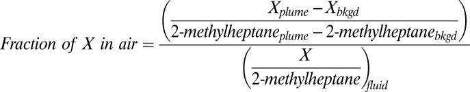The numerator is the slope of a linear regression to X and 2-methylheptane measured in the atmosphere, and the denominator is the mass abundance of X relative to 2-methylheptane in the leaking fluid (5). Here, we normalize to 2-methylheptane, but the results are insensitive to the choice of undissolved and volatile hydrocarbon for the denominator. The present analysis uses atmospheric hydrocarbon data obtained from ships and the P-3 aircraft between mid-May and the end of June 2010, sampling a much longer time period than the 2 d previously reported (2). The overall picture developed from this larger atmospheric dataset and the leaking fluid composition is qualitatively similar to that reported by Ryerson et al. (2), and is shown graphically in Fig. 2B. The air–water distribution of individual hydrocarbon species reported below is highly constrained by the chemical data; uncertainties of ±10% in the calculated distributions are determined by propagation of gas chromatography-flame ionization detection (GC-FID) calibration uncertainties of ±5% (5, 24). The general similarity of the atmospheric composition, illustrated by data taken over the period of a month, suggests little change in the average composition of the surfacing DWH hydrocarbon mixture during this period.

i) Hydrocarbon mixture remaining subsurface.

DWH hydrocarbon transport into the subsurface resulted from two separate processes operating simultaneously during the spill (8). The first process involved dissolution of hydrocarbons from large, millimeter-scale diameter buoyant droplets during ascent to the surface. Continued buoyant ascent physically transported the resulting droplets out of the trapped intrusion (8), leaving behind dissolved hydrocarbons in the subsurface. The dissolved hydrocarbon composition is determined from observed differences between atmospheric DWH plume composition measured from surface ships and aircraft (2) and the leaking composition measured directly in the well (5). Dissolved mass fractions are given by (1 − fraction of X in air) for compounds more soluble than 2-methylheptane, and they are set to zero for less soluble species (Fig. 2B, Upper, filled red squares). Multiplying these mass fractions by leaking fluid mass abundances gives the dissolved mixture composition, which accounted for ∼25% of the mass of the leaking mixture. Methane (CH₄), ethane (C₂H₆), propane (C₃H₈), and isomers of butane (C₄H₁₀) accounted for 89% of the dissolved hydrocarbon mass.

The second process transporting hydrocarbons into the persistent subsurface plumes involved physical trapping of small droplets of leaking hydrocarbon fluid (8). Trapped small droplets are expected to remain suspended following loss of dissolved hydrocarbons into the surrounding seawater (8). We focus on the deep plume data because subsurface samples (5, 14, 16–22) show little evidence for substantial hydrocarbon mass initially deposited at depths above 1,000 m or below 1,300 m. The relative contribution from (a) dissolved hydrocarbon mass and (b) suspended droplet mass in the deep plume is estimated by comparing subsurface plume chemical composition data with the composition of the unmodified leaking fluid and with its dissolved fraction below.

The deep plume composition is identical to that of the leaking fluid for the highly soluble species but begins to differ for less soluble species. Published subsurface data on alkanes larger than propane, and on aromatics larger than toluene (14–17), were examined for samples within 5 km of the well and for which measured methane was >45,000 nM of seawater or measured toluene was >1,000 ng/μL of seawater. These concentrated near-field plume measurements (Fig. 3 A–C, blue squares) are normalized to the most soluble measured compound and compared with the compositions of dissolved (red circles) and leaking (gray bars) mixtures defined above. In each published dataset, the observed pattern of subsurface hydrocarbons relative to measured methane reported by Joye et al. (17) (Fig. 3A), benzene reported by Camilli et al. (14) (Fig. 3B), or toluene reported by Hazen et al. (16) (Fig. 3C), respectively, approximates the composition of just the dissolved fraction of the leaking mixture. The deep persistent subsurface plumes were primarily composed of dissolved species and were relatively depleted in the more sparingly soluble species. This finding, based on subsurface chemical measurements, is qualitatively consistent with a standard oil drop size parameterization (11) in which droplet number decreases exponentially with increasing diameter, suggesting proportionally little mass can be transported in the form of suspended droplets of liquid oil (Fig. S2B).

Fig. 3.

(A) Subsurface near-field plume data (blue) from Joye et al. (table 2 in ref. 17), normalized to measured methane, compared with the composition of leaking gas and oil (gray) and the composition inferred for the mixture dissolved from the promptly surfacing mass (red). The seven most concentrated samples (CH₄ > 45,000 nM) sampled within 5 km of the well were averaged; the isobutane and n-butane data were transposed, and isomer-specific pentane data were apportioned according to their relative abundance in the leaking fluid. (B) As in A using subsurface plume data from Camilli et al. (14) normalized to measured benzene. (C) As in A using subsurface benzene, toluene, ethylbenzene, and total xylenes (BTEX) plume data >5 μg/L seawater from five separate samples (colored lines and markers) reported in Hazen et al. (16) normalized to measured toluene. (D) As in A using subsurface n-alkane plume data >2.5 μg/L seawater from Hazen et al. (16) normalized to measured toluene. The average and range of (0.15 ± 0.10) used to scale the dissolved oxygen (DO) observations are shown by the dashed line and shading, respectively.

However, the actual drop size distributions of the DWH leaks are not known, and may not be well described by this standard parameterization. Because transport in the subsurface is highly dependent on the actual drop size distribution (8), the mass initially suspended in the deep plumes as small droplets of oil remains one of the largest uncertainties in the DWH hydrocarbon budget to date. Initially, suspended droplets are predicted (8), were positively identified by ROV cameras (14), and are qualitatively confirmed by published subsurface enhancements of sparingly soluble polycyclic aromatic hydrocarbons (15, 16). These latter composition measurements, all taken very close to (within 1 km radius of) the leaking well, are not sufficient to quantify hydrocarbon mass transported in the form of suspended droplets. No direct measurements have been presented to quantify this suspended mass to date.

To begin to address this uncertainty, we use chemical data to define the fractional contribution of sparingly soluble compounds relative to dissolved compounds for samples taken in the deep persistent plume. An approximate estimate is afforded by further analysis of published data (16) on C₁₀ to C₃₂ n-alkanes from samples taken within the concentrated deep plume at varying distances from the well (Fig. 3D). These data show a large systematic depletion (by ∼85%) of heavier n-alkanes relative to the highly soluble aromatic compound toluene (C₇H₈), further demonstrating that proportionally little mass was transported into the deep plume in the form of suspended small droplets. Minimal biodegradation in these samples is indicated by (n-C₁₇/pristane) and (n-C₁₈/phytane) ratios (Fig. 3D) similar to those in the leaking fluid. Sparingly soluble n-alkane mass abundances of ∼15% (range of 5–25%; Fig. 3D) in the deep plume relative to the leaking fluid suggests that 31% (range of 13–43%) of the subsurface plume mass can be accounted for by transport of hydrocarbons in the form of initially suspended droplets. We note this conclusion is qualitatively consistent with DWH simulations showing that only small droplets were trapped (8), as well as with extrapolations from standard dispersed oil droplet size parameterizations (Fig. S2B) suggesting that small droplets do not transport the bulk of the mass (11). However, a different drop size distribution could also be consistent with these observations. More accurate size information through the full range of potential drop size diameters is needed to constrain these extrapolations further.

ii) Volatile mixture evaporating to the atmosphere.

Undissolved volatile and semivolatile hydrocarbons evaporate on characteristic time scales of hours to days after reaching the surface (2, 4, 25). The undissolved and volatile hydrocarbon mixture evaporating within 2–3 h of surfacing (2) was determined directly with uncertainties of ±10% (24) using shipborne and airborne measurements of CH₄ through n-C₁₁. The evaporated fraction of unmeasured semivolatile hydrocarbons greater than n-C₁₁ is calculated (Fig. S5A) using the volatility distribution of the oil mixture determined from the chemical composition and the net evaporation measured in the laboratory (4). The sum of volatile and semivolatile masses (Fig. 2B) shows that 14% of the surfacing mixture was both sufficiently insoluble to reach the surface and sufficiently volatile to evaporate from the slick within 1–2 d of surfacing. Because not all the leaked mass reached the surface, a smaller percentage actually evaporated; this amount is quantified below.

Summing the amounts dissolved and evaporated shows that these processes together reduced the mass of hydrocarbons in the surface slick by [1 − (0.75⋅0.86)] = 0.36, or approximately one-third, relative to the slick mass that would have occurred in the absence of these processes. Further evaporation of less volatile compounds likely removed little additional mass from the slick after the second day (26). The evaporating mixture chemical composition is shown graphically in Fig. 4A; n-heptane, n-octane, n-nonane, and methylcyclohexane were the four most abundant hydrocarbons by mass in the evaporating mixture.

Fig. 4.

Evaporated hydrocarbon composition after 2 d (A; blue bars), surface oil slick composition after 2 d (B; black bars), and dissolved hydrocarbon composition (C; red bars). The leaking hydrocarbon composition from CH₄ through n-C₃₉ (black line) is shown in each panel for comparison. (D) Schematic (not to scale) of hydrocarbon mass flows in the marine environment; values are calculated for June 10, 2010, in millions of kilograms per day.

The atmospheric composition data taken aboard surface vessels and the research aircraft, together with the subsurface composition data, demonstrate relatively little variation in evaporating hydrocarbon composition from late May through the end of June, 2010 (Fig. 2B). The F/V Eugenie cruise data were taken before shearing the broken riser pipe on June 2 and installation of the LMRP cap on June 3. The atmospheric data taken subsequently showed no significant change following this event (Fig. 2B), suggesting little change in the composition of the surfacing hydrocarbon mixture as a result of this intervention. The absence of atmospheric CH₄ enhancements associated with any DWH hydrocarbons in these data (Fig. 2B) confirms earlier reports of complete CH₄ dissolution in the subsurface (2, 18, 19, 21, 22, 27) and demonstrates that no emissions of CH₄ to the atmosphere were detected through at least the first 2 mo of the spill. These atmospheric measurements further demonstrate that leaked benzene (C₆H₆) was nearly completely removed in the water column, minimizing its impact at the surface.

iii) Hydrocarbon mixture remaining in the surface oil slick.

Leaked and surfacing hydrocarbons that neither dissolved nor evaporated within the first 1–2 d of surfacing determined the initial composition of the persistent surface oil slick. Slick chemical composition ∼2 d after surfacing is shown graphically in Fig. 4B; n-C₁₇, n-C₁₆, n-C₁₈, and n-C₁₅ were the four most abundant hydrocarbons by mass in the initial surface slick. Slick composition inferred from the airborne and shipborne atmospheric data is qualitatively confirmed by GC-FID analysis of oil samples taken from R/V Endeavor directly in the surface slick 1.5 km horizontally from the well on June 20, 2010 (Fig. S5B, Lower).

3. Composition Data Constrain Mass Flow Along Different Transport Pathways.

The combined datasets are used to estimate the mass flow rates of leaked hydrocarbons along each of the identified transport pathways (Fig. 4D) in early June, 2010, that can be accounted for by the available chemical composition measurements. These are compared with the consensus government estimate of total mass flow from the well, calculated from the official volume flow rate estimate (1) in barrels of liquid oil (Fig. S1, black circles). Total hydrocarbon mass flow rate, including the gas fraction, is calculated by multiplying the government estimate of leaked oil volume flow by 132.2 kg per stock tank barrel of liquid oil and by a mass ratio of [(gas + oil)/oil] = 1.31 ± 0.08 measured at 1 atmosphere and 15.6 °C from the Woods Hole Oceanographic Institution (WHOI) sample of leaking fluid (5) (Fig. S1, red circles).

i) DWH hydrocarbon mass recovered to the surface ship.

Discoverer Enterprise was the only surface ship recovering hydrocarbons in early June, 2010, via the installed LMRP cap (Top Hat no. 4); liquid oil was collected after separation from recovered gas, which was combusted continuously in a flare. Airborne data in the atmospheric CO₂ plume downwind of the flare on June 10 verify, within error limits, gas and oil recovery rates reported for Discoverer Enterprise (2). We use the reported value of 15,402 barrels of liquid oil recovered on June 10, 2010 (13) and a GOR of 1,600 standard cubic feet per stock tank barrel consistent with the leaking fluid composition (5), and estimate a ±10% uncertainty to derive a mass flow of (2.7 ± 0.3) × 10⁶ kg/d of hydrocarbons recovered via the cap on June 10, with the gas fraction flared and the liquid fraction collected in a tanker. Flared gas and recovered oil amounts are shown schematically in Fig. 4D.

ii) Hydrocarbon evaporation to the atmosphere.

The airborne data on June 10, 2010, show a steady-state atmospheric hydrocarbon mass flux of (0.46 ± 0.23) × 10⁶ kg/d (Fig. 4D), which is the sum of the directly measured hydrocarbon mass evaporating within ∼2–3 h of surfacing (2) plus the lesser volatile hydrocarbon mass evaporating within 1–2 d of surfacing as inferred from atmospheric aerosol data (4). The uncertainty of ±50% is primarily attributable to uncertainties in the integration of atmospheric plume hydrocarbon data. These values are indicated in Fig. 4D.

iii) Hydrocarbon flow into the surface oil slick.

An estimate of mass flow into the surface slick is obtained by summing the dissolved and evaporated masses, and subtracting this sum from the initially buoyant plume mass [according to the method of Ryerson et al. (2), from the slope of the linear fit (red line) in Fig. S4B] of (2.0 ± 1.0) × 10⁶ kg/d. This estimate suggests that (1.0 ± 0.5) × 10⁶ kg/d of leaked hydrocarbons was producing the surface slick in early June.

Analysis of airborne remote sensing data from the airborne visible/infrared imaging spectrometer (AVIRIS) instrument overflights suggested a lower limit to the average daily flow into the surface slick of (0.68–1.30) × 10⁶ kg/d (129,000–246,000 barrels of detectable liquid oil remaining on the surface 25 d after the spill began) (28). This value is consistent with the estimate from P-3 in situ measurements, although different amounts of hydrocarbons were being recovered to the surface on these two dates. The flow rate into the slick derived from in situ measurements on June 10, 2010, indicated in Fig. 4B suggests a relatively small fraction, roughly 13% of the total mass escaping the cap and leaking into the subsurface, formed the persistent, visible surface slick. This likely contributed to a low bias in early oil leak rate estimates that relied on visual observations of the surface slick (29).

iv) Hydrocarbon flow into the subsurface plume.

Subsurface hydrocarbon mass is estimated using measurements of dissolved oxygen (DO) deficits in the deep hydrocarbon plumes. Kessler et al. (18, 19) integrated the detected far-field plume DO deficits to estimate a total of (3.5 ± 0.5) × 10¹⁰ mol of oxygen was consumed during bacterial respiration of DWH hydrocarbons, using data generated on research cruises in August through October, 2010, after flow from the well had ceased. They derived a similar value using the observed near-field relationship between DO and the surfactant di-(2-ethylhexyl) sodium sulfosuccinate (DOSS) in the deep plumes (18–20). This deficit in DO was sufficient to respire all emitted DWH methane in the official estimate (1), plus substantial additional mass of nonmethane hydrocarbons (19). A hydrocarbon mass flux into the persistent deep plume of (3.6 ± 0.8) × 10⁶ kg/d averaged over the 83-d spill is calculated by scaling the integrated DO anomaly by the mass of the dissolved compounds (Fig. 2B), by the estimated mass of suspended droplets, and by O₂ respiration stoichiometry appropriate to each hydrocarbon in this mixture (Table S1).

This calculation assumes complete biodegradation to CO₂ of dissolved hydrocarbons, of which methane (18, 19), ethane (21), propane (21), and isomers of butane (17) account for 89% of the mass (Table S1). It further assumes that by the August through September cruise dates, all hydrocarbon mass was biodegraded (Table S1). The biodegraded fraction of hydrocarbons has not been directly measured, and it is likely to have been negligible for the heaviest hydrocarbons; thus, the calculation represents a lower limit to hydrocarbon mass flow into the deep plume. We note that deriving hydrocarbon mass from the observed DO anomaly is sensitive to the assumed composition and extent of biodegradation of the subsurface plume. Error limits encompassing these sensitivities are estimated by assuming a range of 5–25% for the heavy n-alkane fractions (Fig. 3D, shaded region), leading to a range of 13–43% calculated for the plume mass initially transported in the form of suspended oil droplets. Under these assumptions, the calculated mass flow of (3.6 ± 0.8) × 10⁶ kg/d into the subsurface plumes was the primary flow path for leaked DWH hydrocarbons, as shown in Fig. 4D, and was composed primarily of dissolved species.

v) Composition data constrain hydrocarbon release into the environment.

A total DO-removing potential in the deep plume of (0.041 ± 0.008) mol of O₂ per gram of hydrocarbon is calculated (Table S1) from the deep plume chemical composition above. Dividing this into the total integrated DO anomaly of (3.5 ± 0.5) × 10¹⁰ mol of O₂ removed over the 83 d of the spill results in an average daily environmental hydrocarbon release into the water column of (10.1 ± 2.0) × 10⁶ kg/d (Fig. 5 and Table S1). This hydrocarbon mass flow rate based on the available chemical data agrees, within the uncertainties, with the official estimate of environmental release by subtracting recovered amounts from the official average flow rate of (10.2 ± 1.0) × 10⁶ kg/d of gas and oil based on physical and optical data (1).

Fig. 5.

Left-hand bar shows DWH hydrocarbon mass flow, in millions of kilograms for June 10, 2010, along different environmental transport pathways calculated using the chemical composition data. The center bar shows the calculated release into the Gulf averaged over the spill duration, and the right-hand bar shows the official estimate of total hydrocarbon mass flow averaged over the spill duration.

Discussion

Although the totals agree quantitatively, we note that the sum of chemically detected mass flows along individual transport pathways (Fig. 4D) is lower than the average environmental release rate inferred from the DO anomaly. Although the simplified model shown in Fig. 1 is generally consistent with the available subsurface and atmospheric chemical data, it does not rule out additional mass transported outside of the deep plumes but not yet detected in the chemical data. A specific gravity <1 is expected for the mixture remaining after removal of soluble species; thus, dissolution alone is not expected to cause suspended droplets to descend out of the deep plume. A potential transport pathway could instead involve gradual ascent, on time scales of hours to days, after the initial trapping of small hydrocarbon droplets into the deep plume (8), which would distribute the corresponding hydrocarbon mass into a larger volume of the subsurface as a function of rise velocity, and thus droplet size. Absent measured data throughout the full range of permitted drop sizes, a model study is needed to determine what fraction of the total leaked mass could be represented by the size range of initially trapped droplets that subsequently exited the plume on relevant time scales.

Analysis of the chemical data provides an independent estimate of total hydrocarbon mass flow rate against which other estimates based on physical (1, 12) or optical (13, 30) methods can be compared (Fig. 5). Beyond the flow rate, the chemical data provide critical information on initial environmental distribution of the different mixtures resulting from transport of hydrocarbons emitted from the leaking well (e.g., Fig. 4). The information provided by a cooperative subsurface, surface, and airborne chemical sampling program should therefore be an integral part of a systematic response to future deepwater blowouts. Strategic cooperation during a response would significantly improve the ability to quantify leaking mass and environmental impacts of future spills, and would further provide a means to track and quantify the effects of deliberate intervention measures, subsurface dispersant application, and well and sea-floor integrity after cessation of flow. With sufficient advance preparation, joint airborne and subsurface chemical sampling could provide a national rapid-response capability to assess deepwater well leak rates promptly, especially those in remote and Arctic regions (2).

Materials and Methods

Leaking fluid was collected into isobaric gas-tight samplers by ROV from directly within the LMRP (5). Subsequent analyses of the gas and oil composition were conducted in parallel using GC-FID performed by Geomark Research Ltd., Alpha Analytical Laboratory, and the WHOI, with similar results (5).

Atmospheric hydrocarbon samples were acquired by sampling air into evacuated stainless-steel canisters carried aboard three surface vessels, F/V Eugenie, R/V Pelican, and R/V Thomas Jefferson; similar canisters were used on June 8 and 10 during two DWH survey flights of a chemically instrumented NOAA P-3 research aircraft (2). All atmospheric samples taken aboard the vessels and aircraft flights were subsequently analyzed by GC-FID or GC-MS at the University of California at Irvine (24).

References

- 1.McNutt MK, et al. Assessment of Flow Rate Estimates for the Deepwater Horizon/Macondo Well Oil Spill. Flow Rate Technical Group Report to the National Incident Command Interagency Solutions Group. 2011. Available at http://www.doi.gov/deepwaterhorizon/loader.cfm?csModule=security/getfile&PageID=237763. Accessed December 13, 2011.
- 2.Ryerson TB, et al. Atmospheric emissions from the Deepwater Horizon spill constrain air–water partitioning, hydrocarbon fate, and leak rate. Geophys Res Lett. 2011;38(L07803) 10.1029/2011GL0467. [Google Scholar]
- 3.Graham R, et al. Deep Water: The Gulf Oil Disaster and the Future of Offshore Drilling. 2010. National Commission on the BP Deepwater Horizon Oil Spill and Offshore Drilling Report to the President. Available at http://www.gpoaccess.gov/deepwater/deepwater.pdf. Accessed December 13, 2011.
- 4.de Gouw JA, et al. Organic aerosol formation downwind from the Deepwater Horizon oil spill. Science. 2011;331:1295–1299. doi: 10.1126/science.1200320. [DOI] [PubMed] [Google Scholar]
- 5.Reddy CM, et al. Composition and fate of gas and oil released to the water column during the Deepwater Horizon oil spill. Proc Natl Acad Sci USA. 2012;109:20229–20234. doi: 10.1073/pnas.1101242108. [DOI] [PMC free article] [PubMed] [Google Scholar]
- 6.Zheng L, Yapa PD, Chen FH. A model for simulating deepwater oil and gas blowouts—Part I: Theory and model formulation. Journal of Hydraulic Research. 2003;41:339–351. [Google Scholar]
- 7.Leifer I, Luyendyk BP, Boles J, Clark JF. Natural marine seepage blowout: Contribution to atmospheric methane. Global Biogeochem Cycles. 2006;20(GB3008) 10.1029/2005GB002668. [Google Scholar]
- 8.Socolofsky SA, Adams EE, Sherwood CR. Formation dynamics of subsurface hydrocarbon intrusions following the Deepwater Horizon blowout. Geophys Res Lett. 2011;38(L09602) 10.1029/2011GL047174. [Google Scholar]
- 9.Johansen Ø, Rye H, Cooper C. DeepSpill—Field study of a simulated oil and gas blowout in deep water. Spill Science and Technology Bulletin. 2003;8:433–443. [Google Scholar]
- 10.Chen FH, Yapa PD. Estimating the oil droplet size distributions in deepwater oil spills. Journal of Hydraulic Research. 2007;133:197–207. [Google Scholar]
- 11.Delvigne GAL, Sweeney CE. Natural dispersion of oil. Oil & Chemical Pollution. 1988;4:281–310. [Google Scholar]
- 12.Camilli R, et al. Acoustic measurement of the Deepwater Horizon Macondo well flow rate. Proc Natl Acad Sci USA. 2012;109:20235–20239. doi: 10.1073/pnas.1100385108. [DOI] [PMC free article] [PubMed] [Google Scholar]
- 13.Lehr W, Bristol S, Possolo A. Oil Budget Calculator Deepwater Horizon Technical Documentation. Oil Budget Calculator Science and Engineering Team Report to the National Incident Command Interagency Solutions Group. 2010. Available at http://www.restorethegulf.gov/sites/default/files/documents/pdf/OilBudgetCalc_Full_HQ-Print_111110.pdf. Accessed December 13, 2011.
- 14.Camilli R, et al. Tracking hydrocarbon plume transport and biodegradation at Deepwater Horizon. Science. 2010;330:201–204. doi: 10.1126/science.1195223. [DOI] [PubMed] [Google Scholar]
- 15.Diercks A-R, et al. Characterization of subsurface polycyclic aromatic hydrocarbons at the Deepwater Horizon site. Geophys Res Lett. 2010;37(L20602) 10.1029/2010GL045046. [Google Scholar]
- 16.Hazen TC, et al. Deep-sea oil plume enriches indigenous oil-degrading bacteria. Science. 2010;330:204–208. doi: 10.1126/science.1195979. [DOI] [PubMed] [Google Scholar]
- 17.Joye SB, MacDonald IR, Leifer I, Asper V. Magnitude and oxidation potential of hydrocarbon gases release from the BP oil well discharge. Nat Geosci. 2011;4:160–164. [Google Scholar]
- 18.Kessler JD, Valentine DL, Redmond MC, Du M. Response to Comment on “A persistent oxygen anomaly reveals the fate of spilled methane in the deep Gulf of Mexico”. Science. 2011;332:1033. doi: 10.1126/science.1199697. [DOI] [PubMed] [Google Scholar]
- 19.Kessler JD, et al. A persistent oxygen anomaly reveals the fate of spilled methane in the deep Gulf of Mexico. Science. 2011;331:312–315. doi: 10.1126/science.1199697. [DOI] [PubMed] [Google Scholar]
- 20.Kujawinski EB, et al. Fate of dispersants associated with the Deepwater Horizon oil spill. Environ Sci Technol. 2011;45:1298–1306. doi: 10.1021/es103838p. [DOI] [PubMed] [Google Scholar]
- 21.Valentine DL, et al. Propane respiration jump-starts microbial response to a deep oil spill. Science. 2010;330:208–211. doi: 10.1126/science.1196830. [DOI] [PubMed] [Google Scholar]
- 22.Yvon-Lewis SA, Hu L, Kessler J. Methane flux to the atmosphere from the Deepwater Horizon oil disaster. Geophys Res Lett. 2011;38(L01602) 10.1029/2010GL045928. [Google Scholar]
- 23.Whelan J, Eglinton L, Cathles L, III, Losh S, Roberts H. Surface and subsurface manifestations of gas movement through a N-S transect of the Gulf of Mexico. Marine and Petroleum Geology. 2005;22:479–497. [Google Scholar]
- 24.Colman JJ, et al. Description of the analysis of a wide range of volatile organic compounds in whole air samples collected during PEM-tropics A and B. Anal Chem. 2001;73:3723–3731. doi: 10.1021/ac010027g. [DOI] [PubMed] [Google Scholar]
- 25.Fingas M. The evaporation of oil spills: Prediction of equations using distillation data. Spill Science and Technology Bulletin. 1996;3:191–192. [Google Scholar]
- 26.Fingas MF. Studies on the evaporation of crude oil and petroleum products: I. The relationship between evaporation rate and time. J Hazard Mater. 1997;56:227–236. [Google Scholar]
- 27.Valentine DL. Measure methane to quantify the oil spill. Nature. 2010;465:421. doi: 10.1038/465421a. [DOI] [PubMed] [Google Scholar]
- 28.Clark RN, et al. A Method for Quantitative Mapping of Thick Oil Spills Using Imaging Spectroscopy. 2010. USGS Open-File Report 2010-1167. Available at http://pubs.usgs.gov/of/2010/1167/. Accessed December 13, 2011.
- 29.US Geological Survey Deepwater Horizon MC252 Gulf Incident Oil Budget: Government Estimates—Through August 01 (Day 104) 2010. US Geological Survey Report to the National Incident Command. Available at http://www.usgs.gov/foia/budget/08-02-2010...Deepwater%20Horizon%20Oil%20Budget.pdf. Accessed December 13, 2011.
- 30.Crone TJ, Tolstoy M. Magnitude of the 2010 Gulf of Mexico oil leak. Science. 2010;330:634. doi: 10.1126/science.1195840. [DOI] [PubMed] [Google Scholar]
Associated Data
This section collects any data citations, data availability statements, or supplementary materials included in this article.