Using distance correlation and SS-ANOVA to assess associations of familial relationships, lifestyle factors, diseases, and mortality

Abstract

We present a method for examining mortality as it is seen to run in families, and lifestyle factors that are also seen to run in families, in a subpopulation of the Beaver Dam Eye Study. We observe that pairwise distance between death age in related persons is on average less than pairwise distance in death age between random pairs of unrelated persons. Our goal is to examine the hypothesis that pairwise differences in lifestyle factors correlate with the observed pairwise differences in death age that run in families. Szekely and Rizzo [Szekely GJ, Rizzo ML (2009) Ann Appl Stat 3(4): 1236–1265] have recently developed a method called distance correlation, which is suitable for this task with some enhancements. We build a Smoothing Spline ANOVA (SS-ANOVA) model for predicting death age based on four major lifestyle factors generally known to be related to mortality and four major diseases contributing to mortality, to develop a lifestyle mortality risk vector and a disease mortality risk vector. We then examine to what extent pairwise differences in these scores correlate with pairwise differences in mortality as they occur between family members and between unrelated persons. We find significant distance correlations between death ages, lifestyle factors, and family relationships. Considering only sib pairs compared with unrelated persons, distance correlation between siblings and mortality is, not surprisingly, stronger than that between more distantly related family members and mortality. The methodological approach here adapts to exploring relationships between multiple clusters of variables with observable (real-valued) attributes, and other factors for which only possibly nonmetric pairwise dissimilarities are observed.

Multiple studies have reported that, collectively, lifestyle factors, including smoking, low or high body mass index (bmi), low educational attainment, and low socioeconomic status, are associated with earlier mortality. Diseases, such as diabetes, cardiovascular disease, cancer, and chronic kidney diseases, are leading causes of death. Longevity is generally believed to run in families. Furthermore, there is evidence showing that the lifestyle factors all tend to run in families. The goal of this paper is to capture the association of familial relationships, lifestyle factors, diseases, and mortality. It is possible that some of the lifestyle variables may be or turn out to be related to genetic factors. Current research interest involves searches for “longevity genes,” but this work is not related to that quest. We are not assessing to what extent genetics is involved in longevity.

The Beaver Dam Eye Study (BDES) (1) is an ongoing population-based study of age-related ocular disorders. Subjects at baseline, examined between 1988 and 1990, were a group of 4,926 people aged 43–86 years who lived in Beaver Dam, Wisconsin. Many group members have relatives in the study, and pedigree information was collected. Mortality information was updated to March 2011. BDES provides an excellent opportunity to attempt to examine and quantify the above associations.

A pair of landmark papers (2, 3) proposed the distance correlation as a measurement of multivariate independence, and others have recently built upon it (4–7). The method is extremely general in that it is applicable to random vectors of arbitrary and not necessarily equal dimension and only involves Euclidean pairwise distance. If the two variables are sampled from a bivariate normal distribution, the distance correlation behaves very much like Pearson’s correlation coefficient. Because only Euclidean pairwise distances enter, the method may be applied to inherently unobservable variables with only Euclidean pairwise distances observable. The “genetic distances” defined on pairs of persons representing their familial relationships are generally not Euclidean. However, it is shown that the use of genetic dissimilarity in the distance correlation is still validated because the genetic dissimilarity can be well approximated by Euclidean pairwise distances obtained by embedding the subjects into Euclidean spaces through regularized kernel estimation (RKE) (8, 9).

Smoothing Spline ANOVA (SS-ANOVA) models have a successful history for modeling various aspects of BDES data; two examples are refs. 10 and 11. In this study, we focus on modeling the mortality (death ages) of the following form:

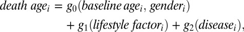where g₀ is a term that involves fixed characteristics, baseline age and gender, for the individuals, g₁ is a term that includes only lifestyle factors, and g₂ is a term containing only disease variables, namely diabetes, cancer, cardiovascular disease, and chronic kidney disease. In the paper, the fitted values of g₁ and g₂ are treated as scores for the individuals and to be used to assess the association with familial relationships.

Pedigrees and Pedigree Dissimilarity

The genetic relationships between pedigree members can be described by Malecot’s (12) kinship coefficient φ, which defines a pedigree dissimilarity measure. The kinship coefficient φ between individuals i and j in the pedigree is defined as the probability that a randomly selected pair of alleles, one from each individual, is identical by descent, that is, they are derived from a common ancestor. For a parent–offspring pair, φ_ij = 0.25 because there is a 50% chance that the allele inherited from the parent is chosen at random for the offspring, and a 50% chance that the same allele is chosen at random for the parent.

Pedigree Dissimilarity.

The pedigree dissimilarity between individuals i and j is defined for this study as d_ij = 1 − 2φ_ij, where φ is the kinship coefficient. Thus, for i ≠ j, the pedigree dissimilarity here falls in the interval . Note that Corrada Bravo et al. (9) define pedigree dissimilarity for that study as −log₂(2φ), which ranges from 1 to ∞ for i ≠ j, which is not appropriate for the way we will be using pedigree dissimilarity.

In BDES, not all family members are included in the study and not all of the subjects have pedigree records.

SS-ANOVA Models

SS-ANOVA models (13–15) estimate the responses y_i, i = 1, …, n to be a function of the covariates f(x_i), by assuming that f is a function in a reproducing kernel Hilbert space (RKHS) of the form = ₀ ⊕ ₁. ₀ is a finite dimensional space spanned by a set of functions {ϕ₁, …, ϕ_m}, and ₁ is an RKHS induced by a given kernel function k(⋅, ⋅) with the property that . Thus, the function f has a semiparametric form of the following:

for some coefficients d_j, where the functions ϕ_j’s are of parametric linear form and g ∈ ₁. ₁ is further decomposed by assuming that it is the direct sum of multiple RKHSs. Hence, g ∈ ₁ is defined to be the following:

where {g_α} and {g_αβ} satisfy side conditions that generalize the standard ANOVA side conditions. Functions g_α are the “main effects” and g_αβ are the “second-order interactions,” and so on. The RKHS _α is associated with each component in the above sum, along with its corresponding kernel function k_α. In this case, the reproducing kernel function for ₁ is defined to be the following:

where the coefficients θ’s are tuning parameters that weigh the relative importance of each term in the decomposition.

The SS-ANOVA estimates f given data {(x_i, y_i), i = 1, …, n} by the solution of a penalized likelihood problem of the following form:

where l(y_i, f(x_i)) = (y_i − f(x_i))² and

with P_αf the projection of f into RKHS _α and λ a nonnegative regularization parameter. The penalty J_λ,θ (f) is a seminorm in RKHS and penalizes the complexity of f using the norm of RKHS ₁ to avoid overfitting f to the training data.

According to Kimeldorf and Wahba (16), the minimizer of the problem in Eq. 1 has a finite representation taking the form of the following:

where for kernel matrix K with K_ij = k(x_i, x_j). Therefore, for a given value of the regularization parameter λ, the minimizer f_λ can be estimated by solving the following convex optimization problem:

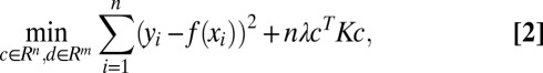where f = [f(x₁), …, f(x_n)]^T = Td + Kc with T_ij = ϕ_j(x_i). The hyperparameters, λ and θ’s, are to be chosen by the generalized cross validation (GCV) (17, 18) method.

Distance Correlation

For a random sample (X, Y) = {(X_k, Y_k): k = 1, …, n} of n independent and identically distributed random vectors (X, Y) from the joint distribution of random vectors X in R^p and Y in R^q, the Euclidean distance matrices (a_ij) = (|X_i − X_j|_p) and (b_ij) = (|Y_i − Y_j|_q) are computed. Define the double centering distance matrices as follows:

where

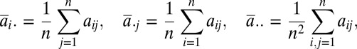similarly for

Sample Distance Covariance.

The sample distance covariance _n(X, Y) is defined by the following:

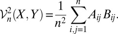Sample Distance Correlation.

The sample distance correlation _n(X, Y) is defined by the following:

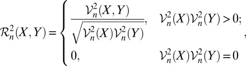where the sample distance variance is defined by the following:

The nonnegativity of and is guaranteed (see ref. 3). The theory in ref. 3 is based on dissimilarities being actual distances between objects embedded in a Euclidean space, although it is mentioned in the rejoinder to the discussion there that the results hold in certain other metric spaces (see also ref. 7). The pedigree dissimilarity (d_ij) cannot be considered as coming from some metric space, however, because, at least in our study, it does not satisfy the triangle inequality. However, we could still treat the pedigree dissimilarity as though it were a distance, because we will see that it can be well approximated by a Euclidean distance obtained by RKE, which we discuss in the next section.

Regularized Kernel Estimation

The RKE framework was introduced in ref. 8 as a robust method for estimating dissimilarity measures between objects from noisy, incomplete, inconsistent, and repetitious dissimilarity data. RKE is useful in settings where object classification or clustering is desired but objects do not easily admit description by fixed-length feature vectors, but instead, there is access to a source of noisy and incomplete dissimilarity information between objects. It estimates a symmetric positive semidefinite kernel matrix K, which induces a real squared distance admitting of an inner product .

Assume dissimilarity information is given for a subset Ω of the possible pairs occurring in a training set of n objects, with the dissimilarity between objects i and j denoted as d_ij ∈ Ω. RKE estimates an n × n symmetric positive semidefinite kernel matrix K of size n such that the fitted squared distance between objects induced by K, , is as close as possible to the square of the observed dissimilarities d_ij ∈ Ω. RKE solves the following optimization problem with semidefinite constraints as follows:

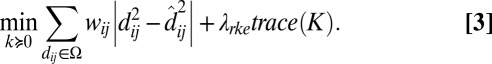The parameter λ_rke ≥ 0 is a regularization parameter that trades off fit of the dissimilarity data, as given by absolute deviation, and a penalty, trace(K), on the complexity of K. The trace may be seen as a proxy for the rank of K. Thus, RKE is regularized by penalizing high dimensionality of the space spanned by K. RKE requires that Ω satisfies a connectivity constraint that the undirected graph consisting of objects as nodes and edges between them, such that an edge between nodes i and j is included if d_ij ∈ Ω is connected. Additionally, optional weights w_ij may be associated with each d_ij ∈ Ω. A method for choosing the regularization parameter λ_rke is required. In this work, λ_rke is fixed at 1. Unlike in many regularization models, results in the RKE tend to be remarkably insensitive to λ_rke over a wide range of values, as can be seen in Fig. 1 of ref. 8.

Fig. 1.

f₃(bmi) (flipped y axis) (Upper) and f₂(edu) + f₁₂(baseage, edu) (Lower) are the fitted effects for bmi and education.

The solution to the RKE problem is a symmetric positive semidefinite matrix K from which an embedding Z ∈ R^n×r in r-dimensional Euclidean space is obtained by decomposing K as K = ZZ^T with , where the n × r matrix Γ_r and the r × r diagonal matrix Λ_r contains the r leading eigenvectors and eigenvalues of K, respectively. The ith row of Z is regarded as the vector of “pseudo” coordinates z(i) for subject i. A method for choosing r is required.

The fact that RKE operates on inconsistent dissimilarity data, rather than distances, fits into pedigree studies significantly where the distance correlation depends on Euclidean distances. The pedigree dissimilarity defined above does not satisfy the triangle inequality for general pedigrees and thus is not Euclidean distance. The Euclidean distances induced by the embedding resulting from RKE provides an approximation of the pedigree dissimilarities in our case. This allows us to validate our result of involving the nonmetric pedigree dissimilarity in distance correlation by comparing with that obtained by using the embedded Euclidean distances.

Beaver Dam Eye Study

The BDES is an ongoing population-based study of age-related ocular disorders. Subjects at baseline, examined between 1988 and 1990, were a group of 4,926 people aged 43–86 years. Pedigree information was available for 2,356 of the subjects. Although we will use data only from the baseline study for our experiments, 5-, 10-, 15-, and 20-year follow-ups were also obtained. Familial relationships of participants were ascertained and pedigrees of different sizes were constructed for the subset of 1,004 subjects who were dead before March 2011 with death ages ranging from 46 to 101 years.

Our goal is to use the data to study the association of familial relationships, lifestyle factors, diseases, and mortality. The strategy is to first estimate the effects of lifestyle factors and diseases on mortality, i.e., death ages, based on the 1,004 subjects using an SS-ANOVA model. The distance correlation is then applied to capture the associations with the estimated effects for a subgroup of 843 people coming from pedigrees containing 2 or more members. This results in 222 pedigrees in the data set, with sizes ranging from 2 to 23 subjects. Note that it is possible for two persons in one pedigree to be genetically unrelated. They become relatives because of their relationships with other members in the pedigree. The pedigree dissimilarity for such a pair is 1 as previously defined.

It is necessary to notice that the covariates can be continuous, binary, and of different magnitude. In addition, the effects of the variables may not be linear in mortality, in which case a large pairwise distance of the covariates values may not result in a large pairwise distance of the death ages. bmi is such an example in that both underweight and obesity are unhealthy and risky to longevity. In this case, the distance of bmi for two individuals, one with low value and the other with high value, is quite large; however, their death age distance may be small. Thus, instead of the original covariates, the estimated effects are preferred in the calculation of distance correlation because the fitted values are naturally assigned with weights and transformations.

For the above purpose, we fit an SS-ANOVA model of the following form:

with variables being described in Table 1 based on 1,004 people. The terms in lines 1, 2 and 3, and 4 and 5 of the above equation are the fixed characteristics, lifestyle factors, and disease variables, respectively. Functions f₁, f₂, and f₃ are cubic splines, and f₁₂ uses the tensor product construction. The remaining covariates are unpenalized and modeled as linear terms with I_{⋅} as indicator functions. The fitted effects for edu and bmi are shown in Fig. 1. The fitted effects of the linear terms are listed in Table 2.

Table 1.

Variable description in the SS-ANOVA model

Variable	Units	Description
deathage	years	Death age
baseage	years	Age at baseline
gender	F/M	Gender
edu	years	Highest year school/college completed
bmi	kg/m2	Body mass index
smoke	Yes/no	History of smoking
inc	Yes/no	Household personal income > 20T
diabetes	Yes/no	History of diabetes
cancer	Yes/no	History of cancer
heart	Yes/no	History of cardiovascular disease
kidney	Yes/no	History of chronic kidney disease

Table 2.

Fitted effects of linear terms in the SS-ANOVA model

Linear term	Fitted effect
Fixed characteristic
gender = F	1.141
Lifestyle Factors
smoke = no	1.349
inc > 20T	0.546
Diseases
diabetes = no	2.000
cancer = no	0.888
heart = no	1.131
kidney = no	1.303

T, Thousand.

Distance correlation, relying on pairwise distances, is the tool for measuring the association among the lifestyle factors, disease variables, mortality, and pedigree. The cohort was restricted to the subgroup of 843 people coming from pedigrees with 2 or more members. Up to now, the pedigree dissimilarities and Euclidean pairwise death age distances are ready for the calculation of the distance correlation. Lifestyle factors and disease variables get involved as the form of lifestyle factor scores and disease scores. The lifestyle factor score for an individual is the vector of the fitted effects for smoke, bmi, edu, and inc. Similarly, the disease score is defined to be the vector of the fitted effects for the four disease variables. The Euclidean pairwise distances of the lifestyle factor scores and disease scores are constructed as the input information for lifestyle factors and disease variables in the distance correlation. Permutation tests are implemented to obtain the p-values of the distance correlations. The network in Fig. 2 summarizes the results. Both mortality and lifestyle factors are associated with familial relationships significantly. Heart disease and some cancers are known to run in families. However, the relationship between pedigree and disease variables in this part of the study is not significant at level 0.05. Included here are some pairs of relatives as distant as second cousins, which may be the cause of the weak signal. However, lifestyle factors, disease variables, and mortality are closely associated with each other.

Fig. 2.

The network of lifestyle factors, disease variables, mortality, and pedigree with distance correlations. The p-values obtained from permutation tests with 1,000 replicates are presented in parentheses. The significance level is distinguished by color: blue for p-value < 0.001, purple for p-value in (0.001, 0.05), and red for p-value > 0.05.

The theory of distance correlation is based on Euclidean pairwise distance. However, three of the above six distance correlations involve the non-Euclidean pedigree dissimilarity. The strategy is to validate the results by showing that the pedigree dissimilarity can be well approximated by Euclidean distances through embedding the subjects in Euclidean spaces by RKE. It is possible to establish the embedding effectively in the RKE framework for a moderate sample size of subjects. However, it is too time consuming to solve the RKE semidefinite problem with the full dissimilarity information for 843 people in our case.

Alternatively, we break down the embedding into two steps. The first step only takes care of the within-pedigree dissimilarity. That is, we feed the familywise pedigree dissimilarities to RKE family by family so that it embeds the subjects into Euclidean spaces pedigree by pedigree. The kernel matrices obtained from RKE are then truncated to those leading eigenvalues that account for 95% of the matrix trace to create the “pseudo”-attribute embedding. The resulting familywise coordinates are put together in a way that each pedigree is assigned its own subspace that is orthogonal to the others. This ends up with a coordinate matrix being a horizontal concatenation of the familywise coordinates. The second step is to take into account of the out-pedigree dissimilarity, which requires pedigree specific variables. We assign one extra dimension to the coordinate matrix for each pedigree. The entries of this extra dimension are the pedigree-specific variable for the family members and 0 for the rest of the subjects. This leads to a coordinate matrix being a function of the pedigree-specific variables. Thus, the augmented coordinate matrix for the rth member in the pth pedigree takes the form of (0, …, 0, v^p, , 0, …, 0), where v^p is the pedigree-specific variable for the pth pedigree and q is the dimension of the subspace for the pth pedigree. The way to choose the pedigree-specific variables is to maximize Pearson’s correlation between the vector form of the double-centered pedigree dissimilarities and the vector form of the Euclidean pairwise distances resulting from the above coordinate matrix. The optimal value of Pearson’s correlation is 0.9907. Fig. 3 shows a comparison of the embedded Euclidean pairwise distances and the pedigree dissimilarities for a subset of 100 subjects. It turns out that the non-Euclidean pedigree dissimilarities are well approximated by the embedded Euclidean distances.

Fig. 3.

The comparison of the Euclidean pairwise distances by embedding and the pedigree dissimilarity for a subset of 100 subjects.

We could establish the distance correlations among the lifestyle factors, disease variables, mortality, and pedigree based on the embedded Euclidean pairwise distances. The results are presented in Fig. 4, where the p-values are also obtained through permutation tests with 1,000 replicates. Both the values of the distance correlation and the p-values are similar to those from the pedigree dissimilarity in Fig. 2. The embedded results are slightly weaker than the original ones due to the shrinkage of RKE by penalizing high dimensionality of the space spanned by the kernel.

Fig. 4.

The network of lifestyle factors, disease variables, mortality, and pedigree with distance correlations using the embedded Euclidean distances. The p-values obtained from permutation tests with 1,000 replicates are presented in parentheses.

In addition to the study of all relatives, the analysis focusing on the full siblings shows that the signal of running in families gets stronger as the familial relationships become closer. The cohort are further restricted to 462 subjects who had at least one full sibling in the group of 843 people. To simplify the procedure, we change the pedigree dissimilarity for the full-sibling pairs, which is shown to be Euclidean. The pedigree dissimilarity is assigned to be 0 for two full siblings and 1 for two unrelated persons. Suppose the subjects who are full siblings to each other are collected to different clusters and there are in total m such clusters. The members in the ith full-sibling cluster are assigned the coordinates of length m, , where the ith element is and the rest are 0. The corresponding Euclidean pairwise distances are unchanged with the above pedigree dissimilarity being defined for full siblings. The distance correlations and p-values are summarized in Fig. 5 for the full-siblings study. The three distance correlation values and related p-values involving familial relationships are strengthened compared with the all-relatives study, indicating that the signal of running in families is getting stronger as the subjects are closer. The other three associations are weaker due to the shrinkage of the sample size.

Fig. 5.

The distance correlations for full-siblings study. The p-values obtained from permutation tests with 1,000 replicates are presented in parentheses.

For the full-siblings study, the pairwise distances for mortality could be separated into two groups, group 0 collecting all of the pairwise death age distances of full-sibling pairs and group 1 for the unrelated pairs. This allows us to compare the difference between the mean of group 1 and the mean of group 0 and construct 95% bootstrap percentile confidence interval (CI) for the test statistic with 10,000 replicates. In the case of mortality, the average death age distance of full-sibling pairs is 1.571 years less compared with that of two unrelated persons in the cohort. The corresponding 95% bootstrap percentile CI for the difference between the mean of group 1 and the mean of group 0 is (0.919, 2.211). We could establish the analysis for the pairwise distances of lifestyle factors and disease variables in the same fashion. The observed test statistics and corresponding CIs are summarized in Table 3. All of the three mean differences between group 1 and group 0 are positive and the CIs do not overlap 0, which means that the full siblings are significantly closer than unrelated people in terms of death age distances, lifestyle factor scores, and disease scores.

Table 3.

Bootstrap percentile CIs for the mean differences in the full-siblings study

Variable	Mortality	Lifestyle	Disease
Group 0 mean	8.091	1.405	1.119
Group 1 mean	9.662	1.654	1.229
Difference	1.571	0.249	0.110
95% CI	(0.919, 2.211)	(0.167, 0.331)	(0.020, 0.202)

Discussion

The BDES, which began collecting data from a population aged 43 and older in 1988, and continues to the present, provides an ideal opportunity to apply some emerging statistical tools to examine questions regarding relationships between various kinds of information collected at the start of the study and mortality. Because the study contains a large number of people with relatives in the study, this provided an ideal opportunity to examine the correlations between familial relationships, lifestyle factors, disease, and mortality. The methodological approach we have proposed here is easily adaptable to other studies for exploring relationships between attributes of subjects with multiple clusters of observable attributes, simultaneously with other factors for which pairwise dissimilarities are observed. Some caveats with respect to the mortality data here are worth mentioning. The mortality data are censored at both ends, that is, we do not see cohorts of the oldest subjects who have died before the study began, and, at the other end, we have access to death ages only to those in the study who have died by March 2011. The left censoring is, to some extent, accounted for in the presence of baseage in the SS-ANOVA model for deathage—note that there is an interaction term for baseage and edu because it was observed that the oldest cohort in the study clearly had fewer years of formal education than younger members. This study does not use the subjects who would otherwise be included who do not have a recorded death age before March 2011. This is, of course, a possible source of bias in the conclusions, and we hope to continue following this group as time goes on. Further research concerning residual lifetimes is ongoing, and the results may be able to use in addition the partial information contributed by subjects that are known to be alive past a particular time. Other information that is not used here includes attributes collected in the follow-up examinations. We cannot in this study exclude possible genetic effects behind the lifestyle factors—we only observe that our lifestyle factors significantly run in families; exactly why is beyond the scope of this project. We have shown that pairwise differences in lifestyle factors that run in families correlate well with pairwise differences in death age that also run in families, partially accounting for the familial death age effect. This leads to new questions to be asked about the complex relationships between genetics, family structure, lifestyle factors, and other variables. We provide here an overall methodological approach that shows promise to help in answering these questions.

Materials and Methods

The package gss in R (www.r-project.org) by Chong Gu (Purdue University, West Lafayette, IN) was used for the SS-ANOVA calculations. The R package energy by Gabor Szekely (National Science Foundation, Arlington, VA) was used for the dcor calculations. Further information regarding RKE calculations can be found in ref. 8, and MATLAB code found in Appendix B of the thesis (19).

References

- 1.Klein R, Klein BEK, Linton KL, De Mets DL. The Beaver Dam eye study: Visual acuity. Ophthalmology. 1991;98(8):1310–1315. doi: 10.1016/s0161-6420(91)32137-7. [DOI] [PubMed] [Google Scholar]
- 2.Szekely G, Rizzo M, Bakirov N. Measuring and testing independence by correlation of distances. Ann Stat. 2007;35(6):2769–2794. [Google Scholar]
- 3.Szekely G, Rizzo M. Brownian distance covariance. Ann Appl Stat. 2009;3(4):1236–1265. doi: 10.1214/09-AOAS312. [DOI] [PMC free article] [PubMed] [Google Scholar]
- 4.Nott D, Tran M, Kohn R. Simultaneous variable selection and component selection for regression density estimation with mixtures of heteroscedastic experts. Electron J Stat. 2012;6:1170–1199. [Google Scholar]
- 5.Li R, Zhong W, Zhu L. Feature screening via distance correlation. J Am Stat Assoc. 2012;107(499):1129–1139. doi: 10.1080/01621459.2012.695654. [DOI] [PMC free article] [PubMed] [Google Scholar]
- 6.Khoshgnauz E. 2012. Learning markov network structure using brownian distance covariance. arXiv:1206.6361v1.
- 7.Lyons R. 2011. Distance covariance in metric spaces. arXiv:1106.5758v3.
- 8.Lu F, Keles S, Wright S, Wahba G. A framework for kernel regularization with application to protein clustering. Proc Natl Acad Sci USA. 2005;102(35):12332–12337. doi: 10.1073/pnas.0505411102. [DOI] [PMC free article] [PubMed] [Google Scholar]
- 9.Corrada Bravo H, et al. Examining the relative influence of familial, genetic and environmental covariate information in flexible risk models. Proc Natl Acad Sci USA. 2009;106(20):8128–8133. doi: 10.1073/pnas.0902906106. [DOI] [PMC free article] [PubMed] [Google Scholar]
- 10.Wahba G, Wang Y, Gu C, Klein R, Klein B. Smoothing spline ANOVA for exponential families, with application to the Wisconsin Epidemiological Study of Diabetic Retinopathy. Ann Stat. 1995;23(6):1865–1895. [Google Scholar]
- 11.Gao F, Wahba G, Klein R, Klein B. Smoothing spline ANOVA for multivariate Bernoulli observations, with applications to ophthalmology data, with discussion. J Am Stat Assoc. 2001;96(453):127–160. [Google Scholar]
- 12.Malecot G. Les Mathematiques de L’Heridite. Paris: Masson et Cie; 1948. [Google Scholar]
- 13.Wahba G. 1990. Spline Models for Observational Data, CBMS-NSF Regional Conference Series in Applied Mathematics, (Society for Industrial and Applied Mathematics, Philadelphia), Vol 59.
- 14.Gu C. Smoothing Spline ANOVA Models. New York: Springer; 2002. [Google Scholar]
- 15.Wang Y. Smoothing Splines: Methods and Applications, Monographs on Statistics and Applied Probability. 2011. (Chapman and Hall/CRC, Boca Raton, FL), Vol 121. [Google Scholar]
- 16.Kimeldorf G, Wahba G. Some results on Tchebycheffian spline functions. J Math Anal Appl. 1971;33(1):82–95. [Google Scholar]
- 17.Golub G, Heath M, Wahba G. Generalized cross validation as a method for choosing a good ridge parameter. Technometrics. 1979;21(2):215–224. [Google Scholar]
- 18.Craven P, Wahba G. Smoothing noisy data with spline functions: Estimating the correct degree of smoothing by the method of generalized cross-validation. Numer Math. 1979;31:377–403. [Google Scholar]
- 19.Lu F. 2006. Regularized nonparametric logistic regression and kernel regularization. PhD thesis (Department of Statistics, Univ of Wisconsin, Madison, WI). Technical Report 1124.