Gene regulatory network modeling using literature curated and high throughput data

Abstract

Building on the linear matrix inequality (LMI) formulation developed recently by Zavlanos et al. (Automatica: Special Issue Syst Biol 47(6):1113–1122, 2011), we present a theoretical framework and algorithms to derive a class of ordinary differential equation (ODE) models of gene regulatory networks using literature curated data and microarray data. The solution proposed by Zavlanos et al. (Automatica: Special Issue Syst Biol 47(6):1113–1122, 2011) requires that the microarray data be obtained as the outcome of a series of controlled experiments in which the network is perturbed by over-expressing one gene at a time. We note that this constraint may be relaxed for some applications and, in addition, demonstrate how the conservatism in these algorithms may be reduced by using the Perron–Frobenius diagonal dominance conditions as the stability constraints. Due to the LMI formulation, it follows that the bounded real lemma may easily be used to make use of additional information. We present case studies that illustrate how these algorithms can be used on datasets to derive ODE models of the underlying regulatory networks.

Introduction

The phenotypic expression of a genome, including the response to external stimuli, is a complex process involving multiple levels of regulation. This regulation includes controls over the transcription of messenger RNA (mRNA) and translation of mRNA into protein via gene regulatory networks (GRNs). Advances in microarray and assay technologies are facilitating increasingly large amounts of laboratory data for analysis of these networks. If the network is operating sufficiently close to a steady-state, Gardner et al. (2003) have shown that multiple linear regressions can be applied to this data to derive a linear ordinary differential equation (ODE) model of the form , where x is the vector of gene expression values and u is the exciting input (see Gardner et al. 2003; Tegner et al. 2003). Now, in addition to this data, information on the interactions between genes, proteins, and metabolites is available through published literature. Observing that this information can be included as a constraint in the optimization problem solved in Gardner et al. (2003), Zavlanos et al. (2011) have performed convex relaxations on the modified optimization problem and have given a linear matrix inequality (LMI) based solution to derive linear ODE models of gene regulatory networks. In particular, (Zavlanos et al. 2011) re-formulates the approach of Gardner et al. (2003) using LMI’s and includes sufficient conditions for asymptotic stability, given by the Lyapunov stability theorem (see Desoer and Vidyasagar 1975; Vidyasagar 1993; Sastry 1999), as the additional constraints to ensure that the linear ODE model is stable. In Zavlanos et al. (2011) , the problem formulation and its solution is presented in a highly lucid manner and its choice of LMI formulation is likely to lead to a number of LMI-based solutions for such network modeling problems.

The paper is organized as follows. After stating our modeling assumptions, we present the network modeling algorithms of Zavlanos et al. (2011) and our extensions of those algorithms. We then show that our algorithms perform at least as well as those algorithms when presented with a synthetic dataset that is generated using the procedure given in Zavlanos et al. (2011). We then show how these results can be used to derive a protein regulatory network of malaria infected patients.

Linear ODE models of gene regulatory networks

The problem of how the gene expression data should be used to obtain linear ODE models of the underlying gene regulatory networks has been well researched (see for example Bansal et al. 2006, 2007; Gardner et al. 2003; Penfold and Wild 2011; Sontag et al. 2004; Tegner et al. 2003, and references therein). We shall focus on deterministic models. The ODE model is of the form , where A and B are real-valued matrices of suitable sizes, x is the vector of gene expression values, and u is the vector (or matrix) of exciting inputs. Laboratory data on the gene expression values for varying inputs furnishes the datasets X and U, where the matrix X comprises the vectors of gene expression values and the matrix U comprises the vectors of corresponding excitations. Now, the objective is to solve for A and B such that some performance metric is optimized. Assuming the availability of time-series data for the gene expression values, such models are derived in Bansal et al. (2006 and 2007) whereas this requirement is relaxed in Gardner et al. (2003), Tegner et al. (2003), and Zavlanos et al. (2011). All of these approaches rest on the assumption that the network is operating sufficiently close to a stable equilibrium point. Under this assumption, solving the ODE for A and B effectively reduces to solving the equation 0 = Ax + Bu for A and B. In addition, it is assumed in Gardner et al. (2003), and therefore in Zavlanos et al. (2011), that the inputs u can be controlled to selectively over-express precisely one gene at a time. This reduces the matrix B to an identity matrix and, as a result, only the matrix A needs to be solved for. However, in practice, such controlled excitation is rarely performed, at least as of today. Instead, most pharmaceutical companies and cosmetic firms have large repositories of snapshots of the gene expression values for the control cases, i.e., for normal subjects, and for the treatment cases, i.e., for the cases in which the subject is either abnormal or exposed to an excitation or a treatment (such as a radiation or a drug dose). Here, it rarely holds that the excitation input u selectively over-expresses (or suppresses) precisely one gene at a time. We shall show that the approach of Zavlanos et al. (2011) is applicable even when its overly restrictive constraint B = I is relaxed.

Method

Assumptions

Our main assumptions are as follows.

• The network can be modeled as for some function f.

• The network has a stable equilibrium point, x_eq, in the neighborhood of which can be approximated as , where , for some matrices A and B.

• The operating point of the network is sufficiently close to the stable equilibrium.

• The matrix A is invariant across all treatments and all subjects.

• The matrix A is sparse (see Arnone and Davidson 1997; Theiffry et al. 1998).

• The input u is to be computed as follows. The exogenous excitation is a transcription perturbation in which individual genes are over-expressed using an episomal expression plasmid. After the perturbation, these cells are allowed to grow under constant physiological conditions to a steady-state and the difference in the mRNA concentrations of these cells and that of normal cells, i.e., those having reporter genes as opposed to the over-expressed genes is to be noted down (see DiBernardo et al. 2004). In general, a perturbation will affect p ≤ n genes in the n-gene network.

• Specific genes encode the transcription factors (TFs)— proteins that can bind DNA (either independently or as part of a complex), usually in the upstream regions of target genes (promoter regions), and so regulate their transcription. Since the targets of a TF can include genes encoding for other TFs, as well as those encoding for proteins of other function, interactions between transcriptional and translational levels of the system take place. In addition, post-translational and epigenetic effects also influence the network. We assume these can be accounted for indirectly in the gene regulatory network.

Background results

Let us now note the main results of Zavlanos et al. (2011). To begin with, let us denote the i-th element of a vector v as v_i and the (i, j)-th element of a matrix A as either a_i,j or a_ij. Let m be the number of available transcription perturbations. Let n denote the number of genes. Let and be the matrices containing transcriptional perturbation values and their associated mRNA expression values, respectively, for the m experiments. Then, if the network modeled as is at the stable equilibrium, then it holds that In general, the measured deviation in x can be different from the deviation predicted by the linear ODE model. Therefore, let , where X comprises the measured values and is the mismatch due to nonlinearities, measurement noise, etc. Then, , where . The network modeling problem can now be stated as follows: Given X and U, determine a sparse stable matrix A that minimizes η subject to the constraint that it satisfies the constraints laid down by a priori information.

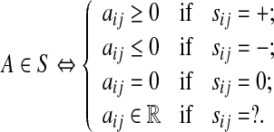
The a priori information is often in the form of sign pattern S that captures the interaction between the nodes i and j. The convention is that s_ij is (i) ’+’ if the node j activates the node i, (ii) ’-’ if the node j inhibits the node i, (iii) zero if the nodes i and j do not interact, and (iv) ’?’ if no a priori information is available on how the node j affects the node i. Then,

1

The stability constraint is satisfied if every eigenvalue of A has a negative-valued real component. Since minimizing might have an adverse effect on η and vice versa, a convex combination of and η is minimized in Zavlanos et al. (2011)—specifically, the Problem 1 is first re-cast as the following optimization problem P1:

where is a user defined parameter. Now, is a non-convex function. Hence, it is relaxed in Zavlanos et al. (2011) to a convex function, namely, a weighted ℓ₁-norm ∑ⁿ_i,j=1w_ij|a_ij|, where the weights w_ij are defined as

2

where δ > 0. If δ is chosen sufficiently small then the value of w_ij |a_ij| ≈ 1 if a_ij ≠ 0 and is zero otherwise. The following algorithm, viz., [20, Algorithm 1], solves this optimization problem.

To ensure that the system is stable, the eigenvalues of A must be constrained to have negative valued real part so that P1 is modified into the following optimization problem P2:

where is a user defined parameter. In Zavlanos et al. (2011), a solution to P2 is obtained by using the Gershgorin’s circle theorem as follows (see Algorithm 2 of (Zavlanos et al. 2011)).

Theorem 1

(Gershgorin’s Circle Theorem (see [Horn and Johnson 1991))] Let . For all   define the deleted absolute row sums of A  as  .  Then, all eigenvalues of A lie within the union G(A) of n discs that is defined as

Furthermore, if a union of k of these  n  discs forms a connected region that is disjoint from every other disc then that region contains precisely k  eigenvalues of 

From Theorem 1, it follows that the matrix A is stable if a_ii ≤  − ∑_i ≠ j |a_ij|   ∀ i, which holds if A is diagonally dominant with non-positive diagonal entries. To relax this restrictive requirement, a similarity transformation V can be applied to A since the eigenvalues of V⁻¹AV are the same as those of A. An easy choice for V is with v_i > 0. Then, using 1, it follows that the matrix V⁻¹AV is stable if Therefore, it follows (see Zavlanos et al. 2011) that the solution A of P2 is guaranteed to be stable if it is obtained by solving the following modified optimization problem P3:

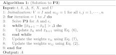
where is a user defined parameter. The matrices V and W can be chosen as follows (see Zavlanos et al. 2011). Initialize V = I where I is the identity matrix of suitable size and set w_ij = 1   ∀ i,j. Then, repeatedly solve P3, updating w_ij using Eq. (2) and v_ii using

3

where .

Remark 1

In Zavlanos et al. (2011), it is claimed that this procedure, described in [20, Algorithm 2], usually requires no more than J = 20 iterations but may yield periodic solutions for certain ill-condition problems.

Remark 2

Zavlanos et al. (2011) (Algorithm 2) is somewhat ad-hoc since the parameter δ is left undefined in it.

Remark 3

In Zavlanos et al. (2011), another solution to P2 is obtained by using the Lyapunov stability theorem to ensure the stability (see Zavlanos et al. 2011, Algorithm 3).

Main results

The values of v_ii in the above algorithm can be updated at the end of each iteration using a number of known results. For example, it is shown in (Mees 1981) that the optimal diagonal postcompensator V to render the matrix VA row dominant can be obtained by computing the left Perron eigenvectors of the nonnegative matrix T having |a_ij| as its elements, provided it is a primitive matrix. Also, it is known that the Perron eigenvalue and its corresponding eigenvector can be easily computed using the following iterative method: select an arbitrary unit vector x₀, then iterate it as follows:

4

until , where is arbitrarily small. Now, is a reasonable approximation of the right perron eigenvector of T, and its corresponding eigenvalue r can be obtained by solving (see Mees 1981). If the column-dominance of A is to be optimized then the same procedure should be applied to A^T and then the result should be transposed. Therefore, Perron eigenvector of T seems to be a good choice for the construction of the scaling matrix V, where

5

Hence, Algorithm 1, an improvement over [Zavlanos et al. 2011, Algorithm 2], can be stated as follows.

Another approach to modify Algorithm Z so that its output A is a stable matrix is as follows (see Zavlanos et al. 2011). If the output A is unstable, perturb it by a small enough perturbation D such that the perturbed matrix is stable and, furthermore, an element of S. By Lyapunov stability theorem, is stable if there exists a P = P^T > 0 such that , i.e., if

6

where . Now, (6) is an LMI that can be efficiently solved by solving the following semidefinite program P4:

the solution of which gives the perturbation as D = P⁻¹L (see Boyd and Vandenberghe 2003). However, while this perturbation ensures the stability of it does not ensure In Zavlanos et al. (2011), this difficulty is resolved by using the Lyapunov matrix P, obtained as a solution of P4, in solving the following optimization problem P5:

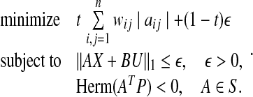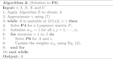
A solution to this problem is given by [20, Algorithm 3].

If the network is sufficiently damped then can be approximated by where G is the transfer function of the linearized system, and y_ss is the steady-state response of the system, which is the same as state vector if C = I_n. Therefore, if sufficient amount of the steady-state data is available then can be approximated as:

7

where the maximization is performed over the experiment trials. Now, the well-known bounded real lemma (BRL) can be used to derive a more powerful network modeling algorithm.

Theorem 2

(Bounded Real Lemma (Apkarian et al. 1996) ) Let the system  G(s) be given in the state-space form as

Then, A is stable and  if and only if the system of LMI’s:

has a symmetrix matrix P as its solution.

Therefore, we can identify out network model by solving the following optimization problem P6:

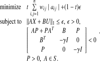A solution to this problem is obtained by using Algorithm 2. In all algorithms considered thus far, the matrix B is assumed to be known. However, as observed earlier, such is rarely the case in practice. If A and B both need to be estimated then more a priori information on A is required since, otherwise, A = 0 and B = 0 is a trivial solution to 0 = Ax + Bu. Such a meaningless solution can be readily ruled out by stipulating a_ii < σ_i   ∀ i for some σ_i as a constraint in the optimization problem. This constraint is valid in reality since every gene and protein down-regulates its own production through self-degradation. Using Gershgorin’s circle theorem to guarantee the stability, the estimation of A and B can be obtained from the solution of the following optimization problem P7:

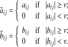
where is a diagonal matrix that has the self-degeneration rates as its diagonal elements. The estimation of B introduces a scaling difficulty: if (A^*, B^*) is a solution of our optimization problem, then (α A^*, α B^*) is also a valid solution for every scalar α that satisfies |α| < 1. In fact, scaling by such an α facilitates smaller modeling errors. This difficulty can be resolved by scaling A and B by a suitable positive number, say κ(A, B), so that the absolute value of the largest element of A becomes equal to 1. Depending on its sign, one can then set the elements having absolute value less than an arbitrary small value such as, say, ν = 10⁻⁴: we refer to these matrices as and (see Algorithm 3). The elements of and are defined as

8

In P4, we solve an optimization problem to find a small perturbation that makes matrix A stable, while minimizing an upper bound of the 2-norm of the difference between AX + BU and (see Zavlanos et al. 2011). If the eigenvectors of A can be estimated well enough then A can be stabilized by perturbing its eigenvalues while keeping its eigenvectors fixed. Hence, a revised optimization problem P8 is as follows:

where is the set of matrices having the canonical structure of the Jordan normal form of A. Now, P can be obtained by solving

9

Then, A and B can be computed by solving P7 iteratively.

Now, suppose our experimental data can be partitioned into q separate sets of data, X_i’s, and each set contains the response of our network to the same input value. Therefore, we have

10

where m_i > 0 is the number of data columns in each set, ∑^q_i=1m_i = m, and all columns of U_i’s are the same. Now, if we construct matrix with columns equal to one arbitrarily column chosen from X_i, it holds that

Therefore, we can claim that X′ = ∪^q_i=1 (X_i − X_i0) approximately spans the subspace corresponding to the eigenvectors corresponding to the small eigenvalues of A. As a result, Algorithm Z estimates the eigenvectors of matrix A regardless of its stability. Assuming that the eigenvectors can be estimated well enough, A can be stabilized by perturbing its eigenvalues while keeping its eigenvectors fixed. This gives rise to a revised optimization problem P9 presented below:

11

where is the set of matrices having the canonical structure of the Jordan normal form of A. Now, we can derive the positive definite Lyapanov matrix P by solving Eq. (9) and then compute A and B by solving P7 iteratively. This solution is implemented in Algorithm 4.

Results and discussion

Comparison of our algorithms with the algorithms derived in Zavlanos et al. (2011)

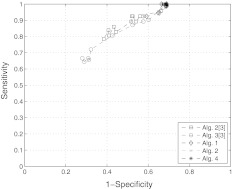
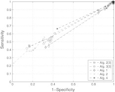
We now present a brief case-study that compares the performance of our algorithms with that of the algorithms presented in Zavlanos et al. (2011) for the same synthetic dataset. For this comparison, a wide range of the parameter t is chosen. To provide results consistent with the ones given in Zavlanos et al. (2011), the receiver operating characteristic (ROC) curves are used as the performance measures. Following (Zavlanos et al. 2011), we define sensitivity and specificity as follows:

Clearly, an identification with 100% sensitivity and specificity is the best possible result. We used the method described in Sect. 5 of Zavlanos et al. (2011) to generate the 20 × 20 random sparse matrix A, and its associated dataset X as X =  − A⁻¹BU + ν N where and are zero mean and unit variance normally distributed random matrices. Then, we identified the system from both full datasets and partial datasets for several values of t. For the case of full dataset, the number of samples are equal to the dimension of the system matrix, i.e., m = n, the noise coefficient is ν = 10%, and a priori knowledge is available for 30% of the matrix entries. For the case of partial dataset, no a priori knowledge is available, the noise coefficient is ν = 50%, and the number of samples is roughly one third of the dimension of matrix A. The results are shown in Figs. 1 and 2. The simulation results show that our algorithms perform at least as well as the ones derived in Zavlanos et al. (2011): the improvement is not surprising since besides reducing the conservatism in the stability constraint used in Zavlanos et al. (2011), we have not altered the structure of the algorithms (Zavlanos et al. 2011) by a great extent.

Fig. 1.

ROC plots for the case of full data, ROC plots of different algorithms for a network of size n = 20 and connectivity c = 20 % using full data (m = n, σ = 30 % and ν = 10 %)

Fig. 2.

ROC plots for the case of partial data, ROC plots of different algorithms for a network of size n = 20 and connectivity c = 20 % using partial data and ν = 50 %)

Illustrative example: GRN for malaria patients

Malaria is a mosquito-borne infectious disease caused in humans and other animals by eukaryotic protists of the genus Plasmodium. Five species of Plasmodium can infect humans with this disease. Among these, the infection from Plasmodium falciparum can be fatal. The infection caused by others, including Plasmodium vivax, is rarely fatal. We now reconstruct the gene-protein regulatory network using two sets of expression data on 30 proteins collected from patients suffering from malaria. GeneSpring version 11.5.1 was used to perform the pathway analysis. GeneSpring has its own pathway database wherein the relations in the database were mainly derived from published literature abstracts using a proprietary Natural Language Processing (NLP) algorithm. Additional interactions from experimental data available in public repositories like IntAct were also included in the pathway database of GeneSpring. The list of Entrez IDs corresponding to the proteins was used to find the key interactions involved in Malaria. The data collected from patients infected by Plasmodium falciparum is tagged FM whereas the data was collected from patients infected by Plasmodium vivax is tagged VM. In addition, we collected the expression data for healthy control samples as well. This data is tagged HC. In all, there are 8 sets of data for HC and a combined 8 sets of data for FM and VM.

where , and . As can be seen, we partitioned the data rows into two parts (one with 18 rows and one with 12 rows). The reason is that among the proteins with available differential expression, only 18 are common in the two data sets, therefore, there are 12 proteins in each data set that expressed in only one type of Malaria. Since our objective was to derive a unified network model, we needed a method to somehow integrate these sets of data together. Hence, we used the average expression values of healthy control samples in one data set to replace the expression value data that are not exhibited in another data set. The reason behind what we did is that if a particular protein, for example P 00751, is specific for Falciparum Malaria, it indicates there is no change in expression level in vivax malaria for that specific protein, hence, we can take the same value that is exhibited by healthy controls. Thus, our matrix is:

where represents a matrix with entries equal to the average of elements in the same row of matrix M. Taking each type of Malaria as an independent input to the system, i.e. U_FM = [1 0]^T and U_VM = [0 1]^T, the input matrix corresponding to our dataset X is U = [M₁  M₂  M₃], where is an all-zero matrix, and are given as

Now, we can model the system as . Using the first 29 columns of X, we trained our network model using Algorithm Z and [20, Algorithm 2]. Verification of our results using the remaining columns of our data showed that [20, Algorithm 2] is not working in this case, and generates a very large error which may be caused by the very conservative stability condition laid down by Gershgorin’s Circle Theorem. However, Algorithm [20, Algorithm 3] works properly with a fairly low error of . 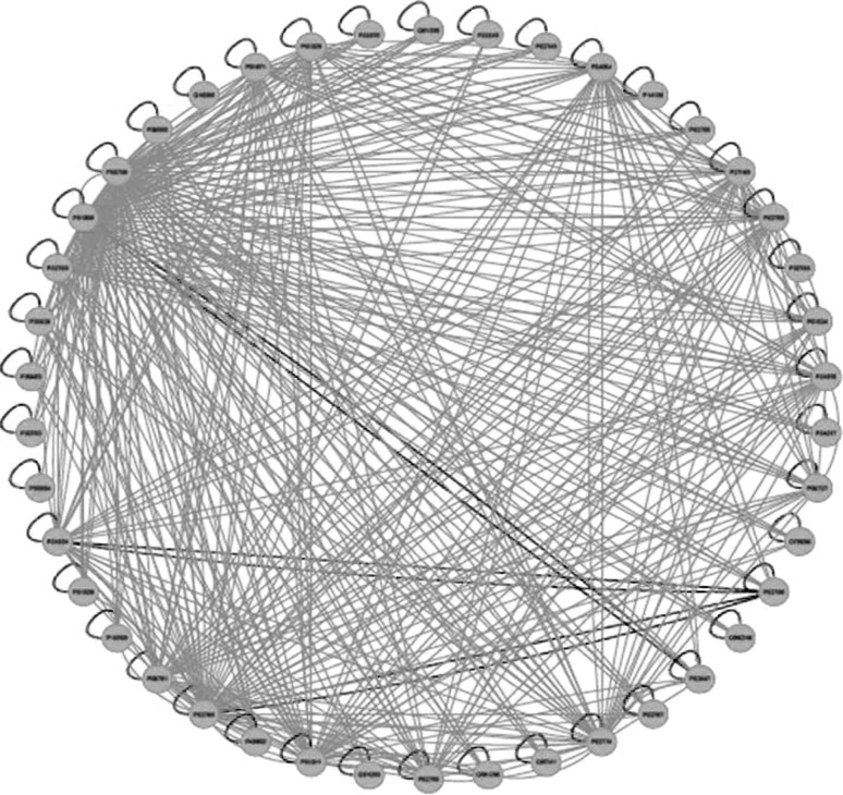We used Cytoscape (see Smoot et al. 2011) to visualize the matrix as a network of interactions. Interactions between all proteins in the matrix were specified in the Simple Interaction File (sif) format and were given to Cytoscape as the input. The SIF file lists each interaction using a source node, a relationship type (or edge type), and the target node. For example, for proteins P1 and P2, the structure P1 1 P2 represents the relationship P1 activates P2 and the structure P1 −1 P2 represents the relationship P1 inhibits P2. The edges in the resulting network are colored by their interaction - a green edge represents activation and a red edge represents inhibitory interaction between the proteins. A representative network diagram is shown in Fig. 3.

Fig. 3.

Gene-protein regulatory network for malaria infected subjects, the gene-protein regulatory network in malaria affected patients. The network has 30 nodes. GeneSpring version 11.5.1 was used to perform the pathway analysis in data collected from hospital patients. Then, our algorithms to obtain linear ODE models of the form were run on the data. This diagram illustrates the network interconnection, determined by the matrix A, and is created using Cytoscape. Green edges represent activation whereas red edges represent inhibition

Conclusion

We have presented a theoretical framework, and associated algorithms, to obtain a class of nonlinear ordinary differential equation (ODE) models of gene regulatory networks assuming the availability of literature curated data and microarray data. We build on a linear matrix inequality (LMI) based formulation developed recently by Zavlanos et al. (2011) to obtain linear ODE models of such networks. However, whereas the solution proposed in Zavlanos et al. 2011) requires that the microarray data be obtained as the outcome of a series of controlled experiments in which the network is perturbed by over-expressing one gene at a time, this requirement is not necessary to implement our approach. We have shown how the algorithms derived in Zavlanos et al. (2011) can be easily extended to derive the required stable linear ODE model. In addition, we have built on these algorithms by using new stability constraints that ensure the diagonal dominance of a given matrix: our case study on a synthetic dataset shows that our algorithms perform at least as well as those given in Zavlanos et al. (2011). We have then presented a case-study of how these algorithms can be applied to derive a protein regulatory network model of malaria-infected patients. Our approach to network reconstruction differs from that of Yuan et al. (2010) in that (Yuan et al. 2010) needs a large number of data samples that are in either a cue-response form or in a time-series form. Our approach to network reconstruction differs from that of Sontag (2008) in that (Sontag 2008) mandates that the data samples should be the outcomes of independent perturbations to the so-called modules of the network. We have implemented our algorithms in MATLAB to successfully reconstruct a sparse 35-node network in which the maximum number of nodes adjacent to a node is 9 (Table 1).

Table 1.

Notation

Symbol	Meaning
	Set of all (nonnegative) real numbers
	n-dimensional (n × m) real-valued vector (matrix)
	n × m real-valued matrix
	Set of all complex numbers
	Set of all integers
or	Transpose of a vector or a matrix
	(Hermitian of )
	Union of the n sets Xi
Xi ∩ Xj	Intersection of the sets Xi and Xj
A ≥ 0 (A < 0)	A is positive semidefinite (negative definite).
	if z is a vector if z is a matrix)
	Number of nonzero elements of (cardinality)
λi(A)	i-th eigenvalue of the matrix A
diag(ai)	Diagonal matrix with ai as its diagonal elements
	=dx/dt (derivative of x with respect to time)

References

- Apkarian P, Becker G, Gahinet P, Kajiwara H (1996) LMI techniques in control engineering from theory to practice. In: Workshop notes—IEEE conference on decision and control, Kobe, Japan
- Arnone M, Davidson E. The hardwiring of development: organization and function of genomic regulatory systems. Development. 1997;124:1851–1864. doi: 10.1242/dev.124.10.1851. [DOI] [PubMed] [Google Scholar]
- Bansal M, Belcastro V, Ambesi-Impiombato A, di Bernardo D (2007) How to infer gene networks from expression profiles. Mol Syst Biol 3(78). doi:10.1038/msb4100120 [DOI] [PMC free article] [PubMed]
- Bansal M, Gatta G, di Bernardo D (2006) Inference of gene regulatory networks and compound mode of action from time course gene expression profiles. Bioinformatics 22(7):815–822. doi:10.1093/bioinformatics/btl003. http://bioinformatics.oxfordjournals.org/content/22/7/815.full [DOI] [PubMed]
- Boyd S, Vandenberghe L. Convex optimization. Cambridge: Cambridge University Press; 2003. [Google Scholar]
- Desoer C, Vidyasagar M. Feedback systems: input-output properties. New York: Academic Press; 1975. [Google Scholar]
- DiBernardo D, Gardner TS, Collins JJ (2004) Robust identification of large scale genetic networks. In: Altman RB, Dunker AK, Hunter L, Jung TA, Klein TE (eds) Biocomputing 2004, proceedings of the Pacific symposium, Hawaii, USA, 6–10 January 2004, World Scientific, pp 486–497 [DOI] [PubMed]
- Gardner TS, Bernardo D, Lorenz D, Collins JJ. Inferring genetic networks and identifying compound mode of action via expression profiling. Science. 2003;301:102–105. doi: 10.1126/science.1081900. [DOI] [PubMed] [Google Scholar]
- Horn R, Johnson C. Topics in matrix analysis. Cambridge: Cambridge University Press; 1991. [Google Scholar]
- Mees A. Achieving diagonal dominance. Syst Control Lett. 1981;1(3):155–158. doi: 10.1016/S0167-6911(81)80029-1. [DOI] [Google Scholar]
- Penfold C, Wild D. How to infer gene networks from expression profiles, revisited. Interface Focus Online. 2011;1(3):857–870. doi: 10.1098/rsfs.2011.0053. [DOI] [PMC free article] [PubMed] [Google Scholar]
- Sastry S. Nonlinear systems—analysis, stability and control. New York: Springer; 1999. [Google Scholar]
- Smoot M, Ono K, Ruscheinski J, Wang P, Ideker T. Cytoscape 2.8: New features for data integration and network visualization. Bioinformatics. 2011;27(3):431–432. doi: 10.1093/bioinformatics/btq675. [DOI] [PMC free article] [PubMed] [Google Scholar]
- Sontag E. Network reconstruction based on steady-state data. Essays Biochem. 2008;45:161–176. doi: 10.1042/BSE0450161. [DOI] [PubMed] [Google Scholar]
- Sontag E, Kiyatkin A, Kholodenko B. Inferring dynamic architecture of cellular networks using time-series of gene expression, protein and metabolite data. BMC Bioinformatics. 2004;20(12):1877–1886. doi: 10.1093/bioinformatics/bth173. [DOI] [PubMed] [Google Scholar]
- Tegner J, Yeung M, Hasty J, Collins JJ (2003) Reverse engineering gene networks: integrating genetic perturbations with dynamical modeling. PNAS 100(10):5944–5949. doi:10.1073/pnas.0933416100. http://www.pnas.org/content/100/10/5944.full [DOI] [PMC free article] [PubMed]
- Theiffry D, Huerta A, Perez-Rueda E, Collado-Vides J. From specific gene regulation to genomic networks: a global analysis of transcriptional regulation in Escherichia coli. Bioessays. 1998;20(5):433–440. doi: 10.1002/(SICI)1521-1878(199805)20:5<433::AID-BIES10>3.0.CO;2-2. [DOI] [PubMed] [Google Scholar]
- Vidyasagar M. Nonlinear systems analysis (Second Edition) Englewood Cliffs: Prentice-Hall; 1993. [Google Scholar]
- Yuan Y, Stan G, Warnick S, Goncalves J (2010) Robust dynamical network reconstruction. In: IEEE conference on decision and control. Atlanta, pp 180–185
- Zavlanos M, Julius A, Boyd S, Pappas G. Inferring stable genetic networks from steady-state data. Automatica: Special Issue Syst Biol. 2011;47(6):1113–1122. [Google Scholar]