“Toward a Clearer Definition of Confounding” Revisited With Directed Acyclic Graphs

Abstract

In a 1993 paper (Am J Epidemiol. 1993;137(1):1–8), Weinberg considered whether a variable that is associated with the outcome and is affected by exposure but is not an intermediate variable between exposure and outcome should be considered a confounder in etiologic studies. As an example, she examined the common practice of adjusting for history of spontaneous abortion when estimating the effect of an exposure on the risk of spontaneous abortion. She showed algebraically that such an adjustment could substantially bias the results even though history of spontaneous abortion would meet some definitions of a confounder. Directed acyclic graphs (DAGs) were introduced into epidemiology several years later as a tool with which to identify confounders. The authors now revisit Weinberg's paper using DAGs to represent scenarios that arise from her original assumptions. DAG theory is consistent with Weinberg's finding that adjusting for history of spontaneous abortion introduces bias in her original scenario. In the authors' examples, treating history of spontaneous abortion as a confounder introduces bias if it is a descendant of the exposure and is associated with the outcome conditional on exposure or is a child of a collider on a relevant undirected path. Thoughtful DAG analyses require clear research questions but are easily modified for examining different causal assumptions that may affect confounder assessment.

In her 1993 paper, “Toward a Clearer Definition of Confounding,” Weinberg focused on clarifying the definition of a confounder in etiologic studies (1). Specifically, she noted a situation where a variable that did not confound the estimated effect would qualify as a confounder according to commonly applied criteria of the time: The variable was associated with exposure, was associated with the outcome among the unexposed, and was not an intermediate factor between the exposure and the outcome. As an illustrative example, she examined the common practice of adjusting for history of spontaneous abortion when estimating the causal effect of an exposure on the risk of spontaneous abortion. She showed, by example, that under simplified but biologically plausible assumptions, controlling for history of spontaneous abortion could substantially bias the estimated risk ratio.

Since the publication of Weinberg's paper, the use of directed acyclic graphs (DAGs) to identify confounders has become increasingly common. Concurrently, it has become more widely recognized that a variable could appear to be a confounder by some conventional definitions but adjustment for that variable could induce bias (2–9). Numerous published texts provide introductions to DAGs (2–7, 10). In this paper, we assume a basic familiarity with DAGs while revisiting Weinberg's original work, using DAGs to evaluate and expand upon her examples.

ORIGINAL ASSUMPTIONS

History of spontaneous abortion is predictive of pregnancy loss and is often adjusted for in studies of spontaneous abortion (11–13), presumably under the assumption that it serves as a proxy for unmeasured confounders rather than supposing that it causally affects the risk of subsequent spontaneous abortions. Weinberg described a hypothetical study for estimating the effect of an exposure (E) (e.g., smoking) on the risk of spontaneous abortion in a current pregnancy (S₂) (1). The exposure was a risk factor for prior spontaneous abortion (S₁), but S₁ was not an intermediate variable between E and S₂. However, S₁ was associated with the outcome among the unexposed, a commonly applied criterion used to determine whether a variable is a confounder when the target population is the exposed group. Thus, S₁ has often been treated as a confounder.

For simplification, Weinberg limited the example to second pregnancies and assumed that a woman's exposure status remained the same across pregnancies (1). Further, she assumed that E increased the risk of an occult abnormality (A) and that A also was the same across pregnancies. Finally, she assumed that the outcomes (S₁ and S₂) were independent, conditional on A, and that Pr[S_i|E, A] = Pr[S_i|A] for pregnancies i = 1, 2.

THE ORIGINAL DAG

We can use DAGs to represent possible underlying causal relations compatible with the statistical assumptions from Weinberg's paper (1). In order to draw appropriate conclusions from a DAG, it is necessary to assume that the DAG represents the true causal relations and that it is not missing any variable that causes any pair of variables in the graph (5, 7). We consider several DAGs that represent variations in the scenario considered by Weinberg. Our interest is in determining whether different DAGs compatible with the scenario described by Weinberg lead us to the same conclusions she reached originally (1) and whether biologically plausible revisions would cause us to revise those conclusions.

The construction and interpretation of a DAG differs depending on the causal contrast of interest and the hypothesized causal relations. First, we will consider an exposure that occurs prior to both pregnancies (e.g., in utero exposure of the pregnant woman to smoking). Formally, let E represent a dichotomous exposure where 1 indicates exposure and 0 indicates no exposure, and let S₂ represent a dichotomous outcome where 1 indicates that the second pregnancy ended in a loss and 0 indicates that it ended in a birth. Assuming that the target population is the exposed group, let S₂^e=1 represent the outcome of the second pregnancy if all exposed women were exposed and S₂^e=0 represent the outcome of the second pregnancy if all exposed women had instead been unexposed. Then the causal risk ratio would be Pr[S₂^e=1 = 1]/Pr[S₂^e=0 = 1]. In the data, only Pr[S₂^e=1 = 1] would be observed (indicated Pr[S₂ = 1|E = 1]). Pr[S₂^e=0 = 1] would be estimated from the experience of the unexposed group, Pr[S₂ = 1|E = 0]. If the (observed) experience of the unexposed group differed from the (unobserved) experience the exposed group would have had if they had been unexposed, then the estimated effect parameter would be biased. Confounding could exist in the unadjusted estimate or could be introduced by inappropriate adjustment for covariates. In this article, we evaluate several DAGs to determine whether adjustment for S₁ introduces bias. Formally, we assess whether Pr[S₂^e=1 = 1]/Pr[S₂^e=0 = 1] = Pr[S₂ = 1|E = 1, S₁]/Pr[S₂ = 1|E = 0, S₁].

DAG 1A (Figure 1A) is consistent with Weinberg's assumptions and is equivalent to Figure 1b in her original paper (1). It assumes that E causes an underlying abnormality A, which in turn affects risk of spontaneous abortion in both pregnancies (S₁ and S₂). In this DAG, there is no confounding, so Pr[S₂^e=1 = 1]/Pr[S₂^e=0 = 1] = Pr[S₂ = 1|E = 1]/Pr[S₂ = 1|E = 0]. Nevertheless, S₁ would be considered a confounder on the basis of some conventional criteria. S₁ is associated with S₂ through an open path that does not directly involve exposure (S₁ ← A → S₂); S₁ is associated with E because S₁ is a descendant of E; and S₁ is not a causal intermediate or mediator between E and S₂. Given these conditions, the unadjusted effect estimate for E would be expected to differ from the estimate adjusted for S₁, but based on DAG 1A, controlling for S₁ would introduce bias (i.e., Pr[S₂^e=1 = 1]/Pr[S₂^e=0 = 1] ≠ Pr[S₂ = 1|E = 1, S₁]/Pr[S₂ = 1|E = 0, S₁]) as Weinberg stated (1), because S₁ and S₂ are affected by a shared parent (A), which is an intermediate between E and S₂. In a sense, S₁ is a proxy for the intermediate A, so adjusting for S₁ is like imperfectly adjusting for an intermediate and produces a form of bias that has been called overadjustment bias (14). The equations from the original paper are directly relevant to this DAG (1).

Figure 1.

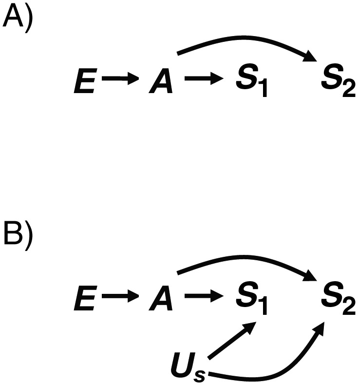
A) Directed acyclic graph (DAG) 1A, in which a single exposure (E) causes a single underlying abnormality (A) that causes both outcomes (S₁ and S₂). B) DAG 1B, in which a shared cause (U_s) of S₁ and S₂ is added to DAG 1A.

One of the advantages of DAG analyses is that one can easily illustrate increasingly complex situations. DAG 1B (Figure 1B) builds on DAG 1A by introducing an unmeasured risk factor for spontaneous abortion (U_s). This addition changes Weinberg's simplifying assumption that S₁ and S₂ are independent conditional on A (1) and is more realistic. Under DAG 1B, Pr[S₂ = 1|E = 1]/Pr[S₂ = 1|E = 0] is still an unconfounded estimate of Pr[S₂^e=1 = 1]/Pr[S₂^e=0 = 1], and Weinberg's conclusion that adjusting for S₁ introduces bias still holds, because adjustment for S₁ would be equivalent to adjusting for a proxy of an intermediate. There are further complications in DAG 1B, because S₁ is also a collider on a path from E to S₂ (E → A → S₁ ← U_s → S₂), so adjusting for S₁ would open this path.

ADDING MULTIPLE EXPOSURES

The DAGs shown in Figure 1 indicate that E and A both occur prior to or during the first pregnancy but affect both pregnancies. For some exposures that do not change (e.g., in utero exposures of the study participant) this might be appropriate, but for an exposure such as participant smoking, which can change, it is important to specify the exact research question. Are we interested in the effect of smoking during the first pregnancy on the outcome of the second pregnancy, or are we interested in the effect of smoking during the second pregnancy on that pregnancy? If the exposure of interest were smoking during the second pregnancy, the DAG would have to be modified to reflect the fact that smoking during the second pregnancy cannot affect the first pregnancy.

The DAGs shown in Figure 2 represent the same exposure (such as participant smoking) at 2 points in time through 2 nodes: E₁ and E₂ (designating smoking during the first and second pregnancies, respectively). In these DAGs, the exposure during each pregnancy produces its own underlying abnormality (such as poor response of the endometrium to pregnancy hormones (1)), which affects only the contemporaneous pregnancy. The new causal risk ratio of interest is .

Figure 2.

A) Directed acyclic graph (DAG) 2A, in which exposure during the first pregnancy (E₁) causes an underlying abnormality during the first pregnancy (A₁) and exposure during the second pregnancy (E₂). E₂ causes an underlying abnormality during the second pregnancy (A₂). In addition, an unknown covariate (U_a) causes both A₁ and A₂, and A₁ and A₂ cause the corresponding outcomes (S₁ and S₂, respectively). B) DAG 2B, in which a shared cause (U_s) of S₁ and S₂ is added to DAG 2A.

Our revised DAGs require us to modify Weinberg's assumptions slightly. The original simplifying assumption that S₁ and S₂ are independent conditional on A is no longer unambiguous, because the abnormality may occur at 2 different points in time. However, we can be consistent with the spirit of the assumption in our revised DAG if S₁ and S₂ are independent conditional on A₁ and A₂. This is the case in DAG 2A, where S₁ and S₂ are not associated through any open paths that do not involve A₁ and A₂ and where conditioning on either would block the otherwise open paths S₁ ← A₁ ← U_a → A₂ → S₂ and S₁ ← A₁ ← E₁ → E₂ → A₂ → S₂. In addition, we now assume Pr[S_i|A_i, E_i] = Pr[S_i|A_i] as an extension of the corresponding original assumption (1). This is represented by the fact that all paths from E_i to S_i go through A_i. Weinberg's assumptions that exposure status and abnormality status are the same for both pregnancies (E₁ = E₂ and A₁ = A₂) are not required to evaluate the revised DAGs and are neither indicated nor contradicted.

In DAG 2A, Pr[S₂ = 1|E₂ = 1]/Pr[S₂ = 1|E₂ = 0] is an unconfounded estimate of because the only backdoor path from E₂ to S₂ (E₂ ← E₁ → A₁ ← U_a → A₂ → S₂) is blocked by the collider A₁. As before, S₁ is not a confounder of the estimated effect of E₂ on S₂, but some conventional criteria would still define it as such. S₁ is associated with the outcome (S₂) among the unexposed because of the open path between them that does not include E₂ (S₁ ← A₁ ← U_a → A₂ → S₂). This path exists because U_a is a shared parent of A₁ and A₂. For concreteness, we can think of U_a as a genetic factor that makes some women liable to develop the abnormality every time they become pregnant. In DAG 2A, S₁ is associated with the exposure of interest (via the open path E₂ ← E₁ → A₁ → S₁) but is not on the causal path of interest (from E₂ to S₂). The association between S₁ and E₂ is due to the assumption in DAG 2A that exposure status during the first pregnancy directly affects exposure status during the second pregnancy (e.g., smoking is addictive, and therefore smokers tend to continue smoking). That is to say, S₁ and E₂ are associated because they share E₁ as a cause.

In DAG 2A, S₁ is neither a confounder nor a child of an intermediate. It meets some conventional criteria for confounding because it is a child of the collider A₁. Adjusting for S₁ will open a backdoor path and bias the effect estimate (i.e., ≠ Pr[S₂ = 1|E₂ = 1, S₁]/Pr[S₂ = 1|E₂ = 0, S₁]). Thus, as Weinberg described in the original paper (1), adjusting for S₁ is not appropriate. The bias introduced by conditioning on S₁ could be removed by conditioning on E₁ or U_a, provided that DAG 2A is correct and complete. However, if the DAG were missing variables, such as a shared cause of S₁ and S₂ (DAG 2B), bias could be introduced by adjusting for S₁ that would not be removed by adjusting for U_a. In addition, adjusting for E₁, a close correlate of the exposure, would affect statistical efficiency.

In DAG 2B, the assumption that S₁ and S₂ are independent conditional on A₁ and A₂ is relaxed by adding an unmeasured shared cause of the pregnancy outcomes (U_s). This creates 2 backdoor paths from E₂ to S₂ (E₂ ← E₁ → A₁ ← U_a → A₂ → S₂ and E₂ ← E₁ → A₁ → S₁ ← U_s → S₂), but both paths are unconditionally blocked by colliders (A₁ and S₁, respectively). Thus, as before, the unadjusted estimate would be an unbiased estimate of the causal contrast, while adjusting for S₁ would open backdoor paths between E₂ and S₂, which would therefore introduce bias.

DAG 3A (Figure 3) is the same as DAG 2A and DAG 3B is the same as DAG 2B, except that in Figure 3 the association between E₁ and E₂ is due to the shared cause U_e (e.g., societal factors that determine smoking behavior) instead of E₁'s directly causing E₂ (i.e., we no longer consider smoking addictive). In both DAG 3A and DAG 3B, as before, the unadjusted estimate for the effect of E₂ on S₂ is unbiased. In DAG 3A, we need not condition on any covariate, because the only backdoor path between E₂ and S₂ (E₂ ← U_e → E₁ → A₁ ← U_a → A₂ → S₂) is blocked by the collider A₁. Once again, S₁ is the child of the collider A₁, so adjusting for S₁ would also open a backdoor path and introduce bias. In DAG 3B, it is inappropriate to adjust for S₁ because it is a collider as well as a child of a collider. This is also true in DAG 3C, which combines DAGs 2B and 3B by allowing E₂ both to be affected by E₁ and to have a shared cause with E₁.

Figure 3.

A) Directed acyclic graph (DAG) 3A, in which an unknown variable (U_e) causes exposure during the first (E₁) and second (E₂) pregnancies. Each exposure causes the corresponding underlying abnormality (A₁ and A₂). In addition, an unknown variable (U_a) causes both underlying abnormalities, and each underlying abnormality causes the corresponding outcome (S₁ and S₂). B) DAG 3B, in which a shared cause (U_s) of S₁ and S₂ is added to DAG 3A. C) DAG 3C, which builds on DAG 3B by allowing E₁ to affect E₂ directly. D) DAG 3D, which builds on DAG 3C by allowing the first outcome (S₁) to affect the second exposure (E₂).

DAG 3D is similar to DAG 3C, but now S₁ is allowed to affect the exposure of interest (E₂). This could occur if a woman modified her behavior based on the outcome of her first pregnancy. For example, a smoker who had a spontaneous abortion during her first pregnancy might quit smoking prior to her second pregnancy. This would violate Weinberg's original assumption that exposure was the same across pregnancies (1). In DAG 3D, there are unconditionally open backdoor paths through S₁ (e.g., E₂ ← S₁ ← U_s → S₂). Thus, this is the first example in which the unadjusted estimate is biased (i.e., ≠ Pr [S₂ = 1|E₂ = 1]/Pr[S₂ = 1|E₂ = 0]). If U_s and U_a were measured, the simplest way to block the backdoor paths would be to condition on them. If they were unmeasured, then conditioning on S₁ would be necessary, but S₁ is a collider on other backdoor paths (E₂ ← E₁ → A₁ → S₁ ← U_s → S₂ and E₂ ← U_e → E₁ → A₁ → S₁ ← U_s → S₂). Therefore, additional adjustment (e.g., adjusting for E₁) would be needed to block the paths opened by conditioning on S₁.

DAGS THAT FURTHER ALTER THE ORIGINAL ASSUMPTIONS

Figure 4 presents DAGs that substantially modify Weinberg's original assumptions (1) despite being similar to the preceding DAGs. DAG 4A is similar to DAG 2A, except that A₁ causes A₂. This modification means that A₁ is no longer a collider, so there is an open backdoor path from E₂ to S₂ (E₂ ← E₁ → A₁ → A₂ → S₂). An unbiased estimate for the effect of E₂ on S₂ would require adjustment for E₁ or A₁. The simplest way to understand this is to note that under this DAG, E₁ is a confounder because it causes both the exposure of interest (E₂) and the outcome (S₂). Theoretically, if neither E₁ nor A₁ were measured, adjusting for S₁ could serve as a proxy for A₁. However, the backdoor path would still remain open to the degree that S₁ was not perfectly correlated with A₁ (7). For DAG 4A, the effect estimate adjusted for S₁ might be less biased than the unadjusted estimate. This conclusion is incompatible with Weinberg's original calculations, because we have modified her assumptions.

Figure 4.

A) Directed acyclic graph (DAG) 4A, in which exposure during the first pregnancy (E₁) causes an underlying abnormality during the first pregnancy (A₁) and exposure during the second pregnancy (E₂). E₂ causes an underlying abnormality during the second pregnancy (A₂). In addition, A₁ causes A₂. Each underlying abnormality causes the corresponding outcome (S₁ and S₂). B) DAG 4B, which removes the effect of A₁ on A₂ that was present in DAG 4A. C) DAG 4C, which alters DAG 4B so that E₁ and E₂ have a shared cause (U_e) instead of E₁ causing E₂.

DAGs 4B and 4C are similar to previous DAGs, except that A_i is only directly affected by E_i. Although these DAGs would initially appear compatible with Weinberg's example (1), they violate the assumption that S₁ and S₂ are associated among the unexposed, because the only path between the two pregnancy outcomes goes through the exposure of interest. Consequently, S₁ would not meet some conventional criteria for a confounder, nor would it be a confounder based on the DAG. If the DAG is correct, if all variables are measured perfectly, if the adjusted model is specified correctly, and if there is no effect-measure modification, adjusting for S₁, although unnecessary, would not bias the effect estimate (i.e., = Pr[S₂ = 1|E₂ = 1]/Pr[S₂ = 1|E₂ = 0] = Pr[S₂ = 1|E₂ = 1, S₁]/Pr[S₂ = 1|E₂ = 0, S₁]) because S₁ is not a risk factor for the outcome. However, adjustment could affect the precision of the estimate (7, 14).

OTHER EXAMPLES FROM THE ORIGINAL PAPER

Weinberg considered other scenarios in which a variable could be mistaken for a confounder (1). She described a general situation where E caused 2 events that were independent given E, and the causal contrast of interest was Pr[S₂^e=1 = 1]/Pr[S₂^e=0 = 1]. The simplest case can be seen in DAG 5A (Figure 5), where the unadjusted estimate of the effect of E on S₂ is not confounded. Nevertheless, as Weinberg reported, no bias would be introduced by adjusting for S₁ because S₁ is not associated with the outcome conditional on E (1, 14). However, in the more realistic scenario where there is a shared cause (U_s) of S₁ and S₂, adjustment for S₁ is no longer benign. DAG 5B is analogous to Figure 1c in the original paper (1). Here again there is no confounding, so Pr[S₂^e=1 = 1]/Pr[S₂^e=0 = 1] = Pr[S₂ = 1|E = 1]/Pr[S₂ = 1|E = 0]; but in this case, adjustment for S₁ induces bias by opening the path E → S₁ ← U_s → S₂. In DAG 5C, however, S₁ is no longer a collider because there is no association between E and S₁, so adjustment for S₁ is unnecessary but would not introduce bias.

Figure 5.

A) Directed acyclic graph (DAG) 5A, in which exposure (E) causes both pregnancy outcomes (S₁ and S₂). B) DAG 5B, which adds a shared cause of S₁ and S₂ (U_s) to DAG 5A. C) DAG 5C, in which E still causes S₂ but no longer causes S₁.

Weinberg also discussed cases where spontaneous abortion might serve as a proxy for an unmeasured confounder (Figure 6). In Figure 5, U_s is not a confounder because it is not unconditionally associated with E, but in Figure 6, U_se is a confounder on a backdoor path from E to S₂. DAG 6A represents a scenario described by Weinberg (1) in which E is unrelated to the risk of S₂ and the unadjusted estimate would be biased because of the open backdoor path E ← U_se → S₂. Adjusting for U_se would block the backdoor path. Although S₁ is not a confounder, it could be used as a proxy for U_se if U_se were unmeasured. However, there would be residual confounding to the degree that U_se and S₁ were not perfectly correlated. In addition, stratifying on S₁ (as Weinberg demonstrated (1)) could result in greater bias in one stratum than in another (7), causing spurious effect-measure modification. DAG 6B is the same as DAG 6A, except that E is allowed to have an effect on S₂. This change would not alter the above conclusions about using S₁ as a proxy for U_se.

Figure 6.

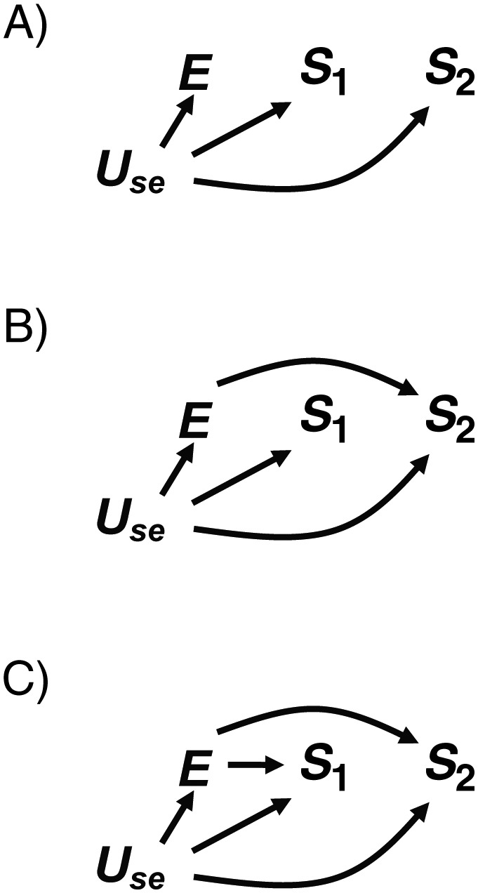
A) Directed acyclic graph (DAG) 6A, in which exposure (E) has no effect on the outcome (S₂). An unmeasured confounder (U_se) is a risk factor for both pregnancy outcomes (S₁ and S₂) and causes E. B) DAG 6B, which builds on DAG 6A by allowing E to be a risk factor for S₂. C) DAG 6C, which builds on DAG 6B by allowing E to affect both pregnancy outcomes (S₁ and S₂).

DAG 6C resembles DAG 6B, except that now E affects both S₁ and S₂. U_se is still a confounder, but S₁ is now a collider, so its ability to serve as a proxy for U_se is compromised. While adjusting for S₁ as a proxy for U_se might be intended to close the backdoor path E ← U_se → S₂, it would open the backdoor path E → S₁ ← U_se → S₂. Whether the effect estimate adjusted for S₁ would be more or less biased than the unadjusted estimate would depend on information not captured in the DAG, such as the strength of the effects represented by each arrow. Thus, for this example, some bias is unavoidable unless U_se is measured.

DISCUSSION

We have used DAGs to revisit the examples Weinberg provided in her landmark 1993 paper, where a variable appeared to be a confounder using commonly applied criteria but adjustment for the variable actually introduced bias (1). Given her assumptions, our conclusions based on several possible DAGs matched those she derived with algebraic examples. To summarize the conclusions of the specific examples we explored, bias may be introduced when a descendant of the exposure is adjusted for if there is a path from that descendant to the outcome that does not involve the exposure (e.g., DAG 1A). Bias also may be introduced by adjusting for a variable that is a collider or a child of a collider on a noncausal path between the exposure and the outcome of interest (e.g., DAG 2A). Both of these situations often plausibly apply to history of spontaneous abortion. Thus, under several different causal structures, bias would be introduced by adjusting for this variable. Even when the true DAG is unknown, it is useful to draw and evaluate several different likely possibilities because, as is illustrated here, the conclusions may be the same under several different causal structures.

History of spontaneous abortion could serve as a proxy for an unmeasured confounder if it is not subject to the conditions just described (e.g., DAG 6B). However, residual bias would remain to the degree that reproductive history was imperfectly associated with the true unmeasured confounder, and this residual bias might be worse in one stratum than in another (7), causing apparent effect-measure modification. Thus, use of reproductive history as a proxy for an unmeasured confounder requires careful consideration.

The DAGs considered here also highlight the importance of defining the specific research question. In Figure 1, we considered an exposure that occurred prior to the first pregnancy outcome, whereas in Figures 2 and 3, we considered an exposure that occurred just prior to the current pregnancy outcome. The evaluation of a potential confounder needs to be made in the context of the specific research question and the associated DAG.

As DAG theory has percolated into epidemiology, there has been increasing awareness of the inadequacy of conventional criteria for appropriately identifying confounders, especially in the case where collider stratification bias may occur (3, 7, 9). DAGs help us build useful etiologic models by providing a transparent way to represent the causal relations between variables. They have simple rules that allow the identification of confounders, and they allow complexity that cannot be illustrated as concisely using algebraic proofs. However, DAGs do not provide information on the magnitude of the effects or the magnitude of the bias introduced by improper exclusion of confounders or inappropriate adjustment for nonconfounders. Quantitative analyses complement DAGs because they can be used to explore the magnitude of these biases under specific assumptions. Nevertheless, in order for a DAG (or an algebraic example) to be effective, the research question must be clearly defined. Even then, both approaches require simplifying assumptions. Despite their limitations, together quantitative sensitivity analyses and DAGs improve our ability to make causal inferences from observational data.

REFERENCES

- 1.Weinberg CR. Toward a clearer definition of confounding. Am J Epidemiol. 1993;137(1):1–8. doi: 10.1093/oxfordjournals.aje.a116591. [DOI] [PubMed] [Google Scholar]
- 2.Greenland S, Pearl J, Robins JM. Causal diagrams for epidemiologic research. Epidemiology. 1999;10(1):37–48. [PubMed] [Google Scholar]
- 3.Greenland S. Quantifying biases in causal models: classical confounding vs collider-stratification bias. Epidemiology. 2003;14(3):300–306. [PubMed] [Google Scholar]
- 4.Hernán MA, Hernández-Díaz S, Werler MM, et al. Causal knowledge as a prerequisite for confounding evaluation: an application to birth defects epidemiology. Am J Epidemiol. 2002;155(2):176–184. doi: 10.1093/aje/155.2.176. [DOI] [PubMed] [Google Scholar]
- 5.Hernán MA, Hernández-Díaz S, Robins JM. A structural approach to selection bias. Epidemiology. 2004;15(5):615–625. doi: 10.1097/01.ede.0000135174.63482.43. [DOI] [PubMed] [Google Scholar]
- 6.Pearl J. Causal diagrams for empirical research. Biometrika. 1995;82(4):669–710. [Google Scholar]
- 7.Glymour MM, Greenland S. Causal diagrams. In: Rothman KJ, Greenland S, Lash TL, editors. Modern Epidemiology. 3rd. Philadelphia, PA: Lippincott Williams & Wilkins; 2008. pp. 183–209. [Google Scholar]
- 8.Shpitser I, VanderWeele TJ, Robins JM. Proceedings of the 26th Conference on Uncertainty and Artificial Intelligence. Corvallis, WA: AUAI Press; 2010. On the validity of covariate adjustment for estimating causal effects; pp. 527–536. [Google Scholar]
- 9.Hernández-Díaz S, Schisterman EF, Hernán MA. The birth weight “paradox” uncovered? Am J Epidemiol. 2006;164(11):1115–1120. doi: 10.1093/aje/kwj275. [DOI] [PubMed] [Google Scholar]
- 10.Pearl J. Causality: Models, Reasoning, and Inference. 2nd. New York, NY: Cambridge University Press; 2009. [Google Scholar]
- 11.Nelson DB, McMahon K, Joffe M, et al. The effect of depressive symptoms and optimism on the risk of spontaneous abortion among innercity women. J Womens Health (Larchmt) 2003;12(6):569–576. doi: 10.1089/154099903768248276. [DOI] [PubMed] [Google Scholar]
- 12.Swan SH, Waller K, Hopkins B, et al. A prospective study of spontaneous abortion: relation to amount and source of drinking water consumed in early pregnancy. Epidemiology. 1998;9(2):126–133. [PubMed] [Google Scholar]
- 13.Weng X, Odouli R, Li DK. Maternal caffeine consumption during pregnancy and the risk of miscarriage: a prospective cohort study. Am J Obstet Gynecol. 2008;198(3):e1–e8. doi: 10.1016/j.ajog.2007.10.803. [DOI] [PubMed] [Google Scholar]
- 14.Schisterman EF, Cole SR, Platt RW. Overadjustment bias and unnecessary adjustment in epidemiologic studies. Epidemiology. 2009;20(4):488–495. doi: 10.1097/EDE.0b013e3181a819a1. [DOI] [PMC free article] [PubMed] [Google Scholar]