Adaptive control of the false discovery rate in voxel‐based morphometry

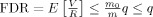
Abstract

Voxel‐based morphometry (VBM) is widely used as a high‐resolution approach to understanding the relationship between anatomical structures and variables of interest. Controlling for the false discovery rate (FDR) is an attractive choice for thresholding the resulting statistical maps and has been commonly used in fMRI studies. However, we caution against the use of nonadaptive FDR control procedures, such as the most commonly used Benjamini–Hochberg procedure (B‐H), in VBM analyses. This is because, in VBM analyses, specific risk factors may be associated with volume change in a global, rather than local, manner, which means the proportion of truly associated voxels among all voxels is large. In such a case, the achieved FDR obtained by nonadaptive procedures can be substantially lower than the nominal, or controlled, level. Such conservatism deprives researchers of power for detecting true associations. In this article, we advocate for the use of adaptive FDR control in VBM‐type analyses. Specifically, we examine two representative adaptive procedures: the two‐stage step‐up procedure by Benjamini, Krieger and Yekutieli (2006: Biometrika 93:491–507) and the procedure of Storey and Tibshirani ([2003]: Proc Natl Acad Sci USA 100:9440–9445). We demonstrate mathematically, with simulations, and with a data example that these procedures provide improved performance over the B‐H procedure. Hum Brain Mapp, 2009. © 2008 Wiley‐Liss, Inc.

INTRODUCTION

Voxel‐by‐voxel morphometric analysis of neuroimages is a powerful analytic tool that allows researchers to evaluate how brain structure is related to relevant risk factors and to functional outcomes. For example, exposures to neurotoxicants, such as lead, may cause structural lesions in the brain [Stewart et al.,2006]; aging or neurological disorders may cause changes in neuro‐anatomy [Honea et al.,2005]; and structural differences may explain variations in cognitive ability [Mungas et al.,2005; Van Petten et al.,2004].

Voxel‐based morphometry (VBM) [Ashburner and Friston,2000] is a high‐resolution approach to evaluate such questions. It proceeds by spatially normalizing each subject image to a common reference image while retaining the absolute volumes (or a proxy thereof) as voxel values. Then a linear model (or generalized model) is fit at every voxel which evaluates the relations between independent variables of interest and volume at each voxel. In this way, a VBM analysis simultaneously tests a large number of hypotheses: whether or not the brain volume at each voxel is associated with the variable of interest. The association between volume and a covariate in a VBM study is analogous to the signal in functional MRI (fMRI) studies.

Compared to traditional morphometric analyses that are based on regions‐of‐interest (ROIs), the advantages of VBM are that it is capable of detecting both global and local associations without prior specification of ROIs for analysis; it does not rely on arbitrarily predefined structures (often based on anatomic structural definitions); and it evaluates all brain locations on equal footing. This has led to a proliferation of studies that have applied VBM to evaluate risk factors for volume loss, as well as studies evaluating volume–function relations [Haier et al.,2005; Kaasinen et al.,2005; Riello et al.,2005; Schwartz et al.,2007; Spencer et al.,2006].

There has been little discussion about the issue of multiple‐hypothesis testing as specifically related to VBM. In the context of fMRI studies, previous work has demonstrated that procedures which control the false discovery rate (FDR) have higher power, and the ability to have data‐driven, rather than prespecified fixed thresholds, compared to those which control the family‐wise error rate (FWER) [Genovese et al.,2002; Logan and Rowe,2004; Marchini and Presanis,2004]. The procedure for deriving statistical maps for VBM is similar to that in fMRI studies. However, in fMRI studies, the activation foci are often small and local, whereas in VBM analyses, risk factors may be associated with volume change in a global manner. Here, we use “global” or “local” to describe the extent of the association, or signal: the proportion of truly associated voxels among all voxels being large (global) or small (local). In other words, an association is global when the associated area is extensive relative to the total brain volume. Therefore, the approach for thresholding VBM‐based statistical maps should differ from that from fMRI analyses. In the remainder of this article, we thus focus on FDR rather than FWER for VBM analyses; as declared in the first FDR publication, “the potential for increase in power is larger when more of the hypotheses are nontrue” [Benjamini and Hochberg,1995].

The most commonly used analytic package, SPM, adopts the nonadaptive linear step‐up procedure, the Benjamini and Hochberg (B‐H) procedure [Benjamini and Hochberg,1995; Benjamini and Yekutieli,2001], for controlling FDR. This implicitly assumes a localized association, specifically a large proportion of truly null voxels. However, when structural changes are global (thus a small proportion of truly null voxels), or when the location of the specific affected area is known a priori and the analysis is restricted to that ROI, this procedure is too conservative, and thus results in overcontrol of the FDR and reduced power. In the sections to follow, we demonstrate the superiority of adaptive procedures [Benjamini et al.,2006; Storey,2002,2003] over nonadaptive ones for researchers who wish to control for FDR in VBM analyses. We include mathematical, simulation‐based, and empirical data‐based support to demonstrate why adaptive procedures are more appropriate in this setting.

BACKGROUND

False Discovery Rate

FDR control is a relatively new notion of global error control in multiple testing situations. Compared to FWER, which is the probability of making at least one false rejection among all tests, FDR focuses on the proportion of rejections that are false. It is less conservative and easy to interpret and it offers an objective and data‐driven perspective for thresholding statistical maps. Below we lay out the notations and definitions to be used in this article.

Let m be the total number of voxels for which the hypothesis is being tested. In VBM analyses, voxels for which the null hypothesis is true are referred to as “not associated” (with the variable of interest), as opposed to “associated.” The total number of “not associated” voxels, or null voxels, is m ₀. The total number of truly associated voxels is m ₁. When a significance threshold t is applied, all voxels with P‐values smaller than t are declared associated, i.e., rejected. The total number of rejections is R(t). As summarized in Table I, the above data give rise to four groups of voxels: correctly declared associated S(t), falsely declared associated V(t), correctly declared not associated m ₀ − V(t), and falsely declared not associated m ₁ − S(t). The FDR refers to the expected proportion of falsely declared‐associated voxels among all voxels that are declared associated [Benjamini and Hochberg,1995]:

(1)

Table I.

Classification of voxels, given a significance threshold t

	Declared associated	Declared not associated	Total
Null true: not associated	V(t)	m 0 − V(t)	m 0
Alternative true: associated	S(t)	m 1 − S(t)	m 1
Total	R(t)	m − R(t)	m

The first factor of (1), the expected fraction of false rejections conditioning on any positive finding, is called positive FDR (pFDR) by Storey [2002]. The pFDR can be interpreted as the posterior probability of the null hypothesis being true when it is rejected. In neuroimaging settings, pFDR is a close approximation of FDR: The second factor in (1), under voxel independence, has when m is large, even for very small probabilities of rejection.

Benjamini–Hochberg Procedure

The Benjamini–Hochberg (B‐H) procedure is the first and most commonly used procedure to control FDR [Benjamini and Hochberg,1995]. It offers a single‐stage linear step‐up algorithm for controlling FDR at level q. Let p _i denote the P‐values from the statistical map of m voxels, i = 1, …, m. We order the P‐values in increasing order, p ₍₁₎ ≤ p ₍₂₎ ≤ ··· ≤ p _(m). Let r be the largest i such that

then we reject all voxels whose P‐value is less than p _(r).

The π₀Factor

Benjamini and Hochberg [1995] proved that, by following the above procedure, . Let denote the proportion of null voxels. From the inequality above, it is clear that the B‐H procedure in fact controls the FDR conservatively at π₀ q. This is close to the nominal level of q only if π₀ ≈ 1, that is, the vast majority of voxels are truly null. In neuroimaging, this requires that the set of associated voxels constitutes a very small fraction among all voxels. This is true for many fMRI studies of brain activation, where it is believed, based on functional biology, that there is an extremely localized neuronal activity for many paradigms. However, in the analysis of structural volumes, specific risk factors (e.g., lead, aging) can be associated with volume loss in a relatively large proportion of the brain [Mungas et al.,2005; Stewart et al.,2006]. In such cases, the B‐H procedure overcontrols the FDR by a factor of 1/π₀, resulting in a higher threshold for significance, fewer discovered voxels, and, hence, reduced power. The B‐H procedure below was originally developed based on the assumption of voxel independence, but later it was shown to be valid under certain positive dependence conditions [Storey et al.,2004]. This issue of voxel dependence is expanded upon in the “Discussion” section.

If the null proportion π₀ were known, then the B‐H procedure with q′ = q/π₀ would control the FDR at the desired level q. A number of procedures therefore seek to improve power by incorporating a π₀ or m ₀ estimation step. Two general estimation approaches include using an initial one‐stage procedure to estimate m ₀, referred to as two‐stage step‐up procedures (TSTs), and estimating directly from the P‐value distribution, referred to as Storey's estimators. Below we present one representative procedure within each approach.

Two‐Stage Step‐Up Procedure

The procedure proposed by Benjamini et al. [2006, see definition 6] includes an initial one‐stage procedure to estimate m ₀.

• Step 1: Use the B‐H linear step‐up procedure at level q′ = q/(1 + q). Let r ₁ be the number of rejected hypotheses. If r ₁ = 0 do not reject any hypothesis and stop; if r ₁ = m reject all m hypotheses and stop; otherwise continue.

• Step 2: Let m̂₀ = m − r ₁.

• Step 3: Use the linear step‐up procedure with q* = q′m/m̂₀.

The rationale for the above approach involves solving the inequality

(2)

where V is approximately equal to or less than qRm ₀/m. There are variations to the two‐stage procedure, for example, one proposed by Benjamini and Hochberg [2000] and several others proposed by Benjamini et al. [2006].

All of these procedures can be implemented with basic programming skills.

Storey's Procedure

Storey's procedure estimates m ₀ directly from the P‐value distribution. Define the function I(.) to be 1 if the statement between the parentheses is true, or 0 otherwise. Then, as described in the work of Storey and Tibshirani [2003], the proportion of null voxels can be estimated by

(3)

where λ can be the median P‐value or 0.5 [Storey,2002; Storey and Tibshirani,2003]. The rationale behind this estimation is that the null P‐values should be uniformly distributed between 0 and 1. Expression (3) is the height of this distribution (or the null proportion) if all P‐values greater than λ were from the null. Since there will also be some non‐null P‐values greater than λ, the above estimate should be on expectation greater than or equal to the null proportion. As λ gets closer to 1, more P‐values should come from the null. Storey and Tibshirani [2003] further proposed a cubic spline‐based approach to extrapolate (3) to λ = 1. The corresponding procedure to control FDR at q is as follows:

• 1Calculate for a sequence of λ values, e.g., 0, 0.01, 0.02, …, 0.95.
• 2Fit a natural cubic spline to the above with d = 3.
• 3Let .
• 4Use the linear step‐up procedure with .

This algorithm is more computer‐intensive than the two‐stage step‐up procedure. It is implemented in the package QVALUE (http://faculty.washington.edu/jstorey/qvalue/). Storey's procedures have been frequently applied to high‐throughput genetics and genomics studies [Chesler et al.,2005; Liu et al.,2006; Sahoo et al.,2007]. To our knowledge, it has not yet been used in VBM imaging studies.

Storey et al. [2004, see sidenote] demonstrated that the B‐H procedure is the same as the Storey procedure using λ = 0 to estimate π₀, i.e., using (3)

SIMULATION STUDY

To study and compare the performance of adaptive and nonadaptive procedures, we conducted simulation experiments in two‐dimension space of 64 pixels by 64 pixels. We assume that the shape of the imaged object roughly resembled an axial view of a human brain with cerebral spinal fluid visible at the center: donut‐shaped with an outer radius of 30 pixels and an inner radius of 10 pixels (see Fig. 1). We then assumed that six areas within the donut‐shaped object are associated with a variable of interest. The six areas were evenly spaced in the donut, each circular in shape, with radius r.

Figure 1.

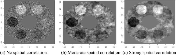
Simulation setup: A statistical map of z‐values is simulated on a donut‐shaped background in two dimensions (the background has an inner diameter of 20 pixels and outer diameter of 60). The mean z‐value in the background is 0. Six circular areas of association have mean z‐values −3, −2, −1, 1, 2, 3. The radius of these areas is set at 5, 7, 8.5, and 10 (shown: 7). Additive noise with standard deviation 1 is generated under three settings: (a) No spatial correlation: Gaussian white noise. (b) Moderate spatial correlation: Gaussian random field noise with a range of 2 pixels. (c) Strong spatial correlation: Gaussian random field noise with a range of 4 pixels.

In each simulation, the corresponding statistical maps were generated as follows: The mean z‐values in these association areas were −3, −2, −1, 1, 2, and 3. Outside the association areas, the z‐values have a zero mean.

To study the effect of spatial correlation on the procedures, we generated noise under three scenarios: (1) no spatial correlation (white noise), (2) moderate spatial correlation, and (3) strong spatial correlation. The spatially correlated noise was generated by a Gaussian random field with a Matérn autocorrelation function [Cressie,1993]. The Matérn autocorrelation function is a flexible parametric form of autocorrelation functions with a smoothness parameter κ and scale parameter ϕ (also referred to as “range”). Both the exponential and Gaussian autocorrelation functions are special cases of Matérn. The former corresponds to κ = 0.5 and the latter to κ = ∞. To simulate dependence that bears resemblance to that in actual statistical maps, we estimated κ and ϕ from statistical maps derived in the real data example later in this article. The estimated κ was 1 (smoothness between exponential and Gaussian) and estimated range ϕ was approximately 2 pixel units (adjusted for resolution). In Scenario 2 moderate correlation, the Gaussian random field noise was generated using κ = 1 and ϕ = 2. In Scenario 3 strong correlation we used κ = 1 and ϕ = 4. In all three scenarios the noise standard deviation was 1. This ensures that the P‐values outside the associated areas are always uniformly distributed. Fitting of the autocorrelation function and Gaussian random field generation were performed using the R package geoR [Diggle et al.,2003; Ribeiro Jr. and Diggle,2001].

To explore a range of values for the null proportion π₀ between 0 and 1, within each scenario, we performed four sets of simulations with the radius of the association areas r being 5, 7, 8.5 and 10, corresponding to decreasing π₀ from 0.81 to 0.25. In each set of simulations, we independently generated 1,000 realizations of the statistical map. We then applied the unadjusted B‐H procedure, the TST, and Storey's cubic spline‐based procedure to control the FDR at q = 0.05.

Table II presents the comparison of the results averaged over the 1,000 realizations. We present three quantities for each simulation: the estimated null proportion , the achieved FDR, and power. Power is defined as the proportion of associated voxels that were correctly identified. In all simulations, all procedures controlled the FDR to be lower than the nominal level of q = 0.05. Out of the three procedures, Storey's procedure always achieved an actual FDR closest to the nominal level, TST the second, and B‐H always the most conservative. The power gain by using Storey's procedure is substantial, especially when π₀ is far from 1. The power gain is lower for TST, suggesting a tendency to be conservative. This can be explained by the adaptive procedures' ability to estimate the null proportion, and by the fact that Storey's procedure offers a better estimate than TST. The conservativeness of TST can also be seen by comparing inequality (2) to Table I: The left side is smaller than the right by m ₁ − S(t), or the proportion of non‐null voxels that are falsely declared as “not associated.” This proportion may not be small when the P‐value distribution under the alternative hypothesis is somewhat diffuse.

Table II.

Results from the simulation study in terms of the achieved false discovery rate and power

Radius (null proportion)	Estimated null proportion			False discovery rate			Power
	B‐Ha	TST	Storey	B‐H	TST	Storey	B‐H	TST	Storey
No spatial dependence
5 (π0 = 0.81)	1	0.97	0.88	0.042	0.044	0.048	0.19	0.20	0.21
7 (π0 = 0.63)	1	0.91	0.76	0.034	0.037	0.044	0.26	0.28	0.30
8.5 (π0 = 0.46)	1	0.85	0.65	0.026	0.031	0.040	0.31	0.33	0.37
10 (π0 = 0.25)	1	0.76	0.52	0.016	0.021	0.031	0.35	0.39	0.45
Moderate spatial dependence
5 (π0 = 0.81)	1	0.97	0.88	0.042	0.043	0.048	0.19	0.20	0.21
7 (π0 = 0.63)	1	0.91	0.76	0.033	0.036	0.044	0.26	0.28	0.30
8.5 (π0 = 0.46)	1	0.85	0.65	0.026	0.030	0.040	0.31	0.33	0.37
10 (π0 = 0.25)	1	0.76	0.52	0.016	0.022	0.032	0.35	0.39	0.45
Strong spatial dependence
5 (π0 = 0.81)	1	0.97	0.87	0.038	0.040	0.048	0.19	0.20	0.21
7 (π0 = 0.63)	1	0.91	0.76	0.030	0.034	0.042	0.26	0.27	0.30
8.5 (π0 = 0.46)	1	0.85	0.65	0.024	0.029	0.039	0.31	0.33	0.37
10 (π0 = 0.25)	1	0.76	0.52	0.016	0.022	0.033	0.35	0.39	0.45

All procedures are performed to control the false discovery rate at α = 0.05. At each prespecified size of the association circles (radius of 5, 7, 8.5, and 10, corresponding to null proportions π₀ of 0.81, 0.63, 0.46, and 0.25), for each of the three procedures, the result is an average over 1,000 realizations.

^aThe Benjamini–Hochberg procedure assumes that the null proportion is always 1.

When r = 10, even at a high noise level compared to the signal, Storey's procedure is powerful enough to detect most of the signals from associated areas with a mean z‐value of −3 and +3, and about half from the −2 and +2 signals. In contrast, the B‐H procedure could only detect the signals at 3 and −3. This demonstrates that, in VBM studies where an exposure causes global volume change, the B‐H procedure will result in a substantial reduction in power, potentially making global volume change appear to be local.

It is worth noting that the performances of all three tests were not much affected by the extent of spatial correlation; the actual FDR and power were very consistent across the three scenarios of little correlation, moderate correlation, and heavy correlation. This provides evidence for the validity of adaptive procedures under positive correlations.

DATA EXAMPLE

In this section, we present a realistic VBM analysis of the association between brain volumes and cognitive function in a group of 510 healthy subjects as part of a large study. It is the first study to use voxel‐based volumetric measures to study the relationship between brain structure and a broad set of cognitive domains on a large number of subjects. All subjects in this study were former lead workers (male, 92.3% are White), with an average age of 56 years (standard deviation 7.7 years) at the time of MRI [Schwartz et al.,2005,2007; Stewart et al.,2006].

Volumetric measures were obtained using the HAMMER spatial registration method that retains absolute volume per voxel [Shen and Davatzikos,2002]. In this method, each scalp‐stripped brain was automatically segmented into anatomically defined ROIs, and then elastically registered to the Talairach stereotaxic coordinate space based on the matching of a collection of geometric attributes. The registration proceeds hierarchically to avoid local maxima during matching. The resulting registration was shown to be anatomically meaningful and highly accurate compared to other existing methods. The original volume was retained as voxel values [Davatzikos,1996; Davatzikos et al.,2001; Shen and Davatzikos,2003]. Cognitive function was measured for each subject within six cognitive domains by their performance in a battery of tests: Domain 1: visuo‐construction; Domain 2: verbal memory and learning; Domain 3: visual memory; Domain 4: executive function; Domain 5: eye‐hand coordination; and Domain 6: processing speed [Schwartz et al.,2000].

Using linear regression of voxel values (volume) on each domain score separately, we obtained six statistical maps of z‐values, accounting for the following covariates: age, first‐time test taker, height, tobacco use, alcohol use, hypertension, diabetes, and education. The hypothesis was tested at each voxel whether a better domain score was associated with a larger volume.

We controlled the proportion of falsely discovered voxels at 0.05 by applying the three procedures examined earlier (the original B‐H procedure, the TST procedure, and Storey's cubic spline‐based procedure) to the statistical maps. Table III presents the total number of discoveries made by each procedure for each cognitive domain, and the associated estimated null proportion . It can be seen that the 's from Storey's procedure were all smaller than 0.50, demonstrating that all cognitive domains (except Domain 2) are associated with brain structure globally, even after adjusting for covariates such as age and height (proxies for total brain volume). In these domains, the TST procedure identified 15–26% more associated voxels than the B‐H procedure, and Storey's procedure discovered 56–147% more voxels than B‐H. This gain of power can also be clearly observed from the three‐dimensional glass brain projection of the association areas identified under each method (see Fig. 2). The TST is fairly conservative compared to Storey's procedure as a result of overestimating π₀.

Table III.

Comparison of real data analysis results for the non‐adaptive Benjamini‐Hochberg (B‐H) procedure, the two‐stage linear step‐up procedure (TST), and Storey's cubic spline‐based procedure (Storey)

Cognitive domain	Number of discovered voxels (million)			Estimated null proportion
	B‐H	TST	Storey	B‐Ha	TST	Storey
D1	1.42	1.74	2.21	1	0.49	0.18
D2	0	0	0	1	1	1
D3	0.81	1.02	1.63	1	0.71	0.28
D4	1.13	1.39	1.86	1	0.60	0.25
D5	0.46	0.53	0.83	1	0.84	0.48
D6	0.43	0.50	1.06	1	0.85	0.39

^aThe B‐H procedure does not estimate the null proportion and assumes it to be 1.

Figure 2.

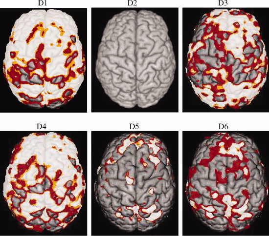
Glass brain projection of the regions associated with six functional cognitive domains on the cortical surface. Three procedures were applied to control the false discovery rate at 5%. Color codes: White: nonadaptive B‐H; Orange + White: Two‐stage procedure TST. Red + Orange + White: Storey's procedure.

DISCUSSION

In this article we introduced the use of adaptive procedures for controlling FDR in VBM studies and showed that they are more powerful than the nonadaptive B‐H procedure. The reason is that these procedures can estimate the proportion of truly null hypotheses π₀, which may be much lower than 1 in VBM studies, while the unadaptive procedure assumes it to be 1. We investigated two approaches that are representative of existing adaptive procedures: the TST by Benjamini et al. [2006] and Storey's cubic spline‐based method (Storey and Tibshirani [2003]). In both the simulation and data example, the adaptive procedures better controlled the FDR while improving power over the B‐H procedure. The power gain is particularly substantial when using Storey's method. It is likely due to a more accurate estimation of π₀. When π₀ is in fact close to 1, all procedures offer similar performance. Thus, the general use of Storey's q‐value procedure seems appropriate in VBM studies.

In both the simulation and the data example, we used a stringent FDR control level of q = 0.05. In the simulation study, this gave rise to powers between 0.19 and 0.45. In other settings, q = 0.10 and 0.20 are frequently used, which will lead to higher power. For example, when controlling FDR at q = 0.20 instead of 0.05, in the case of no spatial dependence, radius of 10 and π₀ = 0.25 (see Table II), the powers of B‐H, TST, and Storey's procedures are 0.58, 0.68, and 0.72 instead of 0.35, 0.39, 0.45, respectively.

The reason that we used a stringent level in this report is because, in VBM studies, many millions of hypotheses are tested simultaneously, where traditional Bonferroni‐type FWER control methods yields extremely low power. Therefore, even a very low q gives tremendous power gain in comparison. Random field theory‐based adjustment to FWER control has been proposed, which increases some power by estimating the number of effective voxels after accounting for spatial correlation [Friston et al.,1991; Worsley et al.,1992]. However, even with the random field theory‐based adjustment, the power of controlling the FWER at 0.05 in the simulation study under any scenario is between 0.01 and 0.05.

It is worth noting that simulations show that the adaptive procedures work well when spatial correlation was present. The B‐H procedure was originally derived under the assumptions that the m ₀ true null hypotheses are independent, and that the m ₀ true null P‐values are uniformly distributed [Benjamini and Hochberg,1995, appendix A), but a later publication [Benjamini and Yekutieli,2001] showed the procedure's validity for finite m for a form of positively dependent P‐values, called “positive regression dependence on subsets.” Storey et al. [2004] proved the validity of both the B‐H and Storey procedures for m → ∞ with some more general forms of weak dependence among the P‐values. However, others have opined [Logan and Rowe,2004] that this assumption may not be met in fMRI datasets. We therefore evaluated the spatial dependence in the statistical maps in our VBM dataset. The original maps containing the volume measures had been smoothed using 10 mm³ FWHM. We found the spatial correlation to be positive between voxels as far as 60 mm apart. The simulation study that reproduced similar and greater spatial correlation (Simulation Scenarios 2 and 3) showed that all procedures are robust in the presence of such correlation.

REFERENCES

- Ashburner J,Friston KJ ( 2000): Voxel‐based morphometry–the methods. Neuroimage 11(6, Part 1): 805–821. [DOI] [PubMed] [Google Scholar]
- Benjamini Y,Hochberg Y ( 1995): Controlling the false discovery rate—a practical and powerful approach to multiple testing. JR Stat Soc Ser B Methodol 57: 289–300. [Google Scholar]
- Benjamini Y,Hochberg Y ( 2000): On the adaptive control of the false discovery fate in multiple testing with independent statistics. J Educ Behav Stat 25: 60–83. [Google Scholar]
- Benjamini Y,Krieger AM,Yekutieli D ( 2006): Adaptive linear step‐up procedures that control the false discovery rate. Biometrika 93: 491–507. [Google Scholar]
- Benjamini Y,Yekutieli D ( 2001): The control of the false discovery rate in multiple testing under dependency. Ann Stat 29: 1165–1188. [Google Scholar]
- Chesler EJ,Lu L,Shou S,Qu Y,Gu J,Wang J,Hsu HC,Mountz JD,Baldwin NE,Langston MA,Threadgill DW, Manly KF, Williams RW ( 2005): Complex trait analysis of gene expression uncovers polygenic and pleiotropic networks that modulate nervous system function. Nat Genet 37: 233–242. [DOI] [PubMed] [Google Scholar]
- Cressie N ( 1993): Statistics for Spatial Data. New York: Wiley. [Google Scholar]
- Davatzikos C ( 1996): Spatial normalization of 3D brain images using deformable models. J Comput Assist Tomogr 20: 656–665. [DOI] [PubMed] [Google Scholar]
- Davatzikos C,Genc A,Xu DR,Resnick SM ( 2001): Voxel‐based morphometry using the RAVENS maps: Methods and validation using simulated longitudinal atrophy. Neuroimage 14: 1361–1369. [DOI] [PubMed] [Google Scholar]
- Diggle P,Ribeiro P Jr,Christensen O ( 2003): An Introduction to Model Based Geostatistics. Spatial Statistics and Computational Methods. Springer. pp 43–86.
- Friston KJ,Frith CD,Liddle PF,Frackowiak RS ( 1991): Comparing functional (PET) images: The assessment of significant change. J Cereb Blood Flow Metab 11: 690–699. [DOI] [PubMed] [Google Scholar]
- Genovese CR,Lazar NA,Nichols T ( 2002): Thresholding of statistical maps in functional neuroimaging using the false discovery rate. Neuroimage 15: 870–878. [DOI] [PubMed] [Google Scholar]
- Haier RJ,Jung RE,Yeo RA,Head K,Alkire MT ( 2005): Structural brain variation, age, and response time. Cogn Affect Behav Neurosci 5: 246–251. [DOI] [PubMed] [Google Scholar]
- Honea R,Crow TJ,Passingham D,Mackay CE ( 2005): Regional deficits in brain volume in schizophrenia: A meta‐analysis of voxel‐based morphometry studies. Am J Psychiatry 162: 2233–2245. [DOI] [PubMed] [Google Scholar]
- Kaasinen V,Maguire RP,Kurki T,Bruck A,Rinne JO ( 2005): Mapping brain structure and personality in late adulthood. Neuroimage 24: 315–322. [DOI] [PubMed] [Google Scholar]
- Liu F,Park PJ,Lai W,Maher E,Chakravarti A,Durso L,Jiang X,Yu Y,Brosius A,Thomas M,Chin L, Brennan C, DePinho RA, Kohane I, Carroll RS, Black PM, Johnson MD ( 2006): A genome‐wide screen reveals functional gene clusters in the cancer genome and identifies EphA2 as a mitogen in glioblastoma. Cancer Res 66: 10815–10823. [DOI] [PubMed] [Google Scholar]
- Logan BR,Rowe DB ( 2004): An evaluation of thresholding techniques in fMRI analysis. Neuroimage 22: 95–108. [DOI] [PubMed] [Google Scholar]
- Marchini J,Presanis A ( 2004): Comparing methods of analyzing fMRI statistical parametric maps. Neuroimage 22: 1203–1213. [DOI] [PubMed] [Google Scholar]
- Mungas D,Harvey D,Reed BR,Jagust WJ,DeCarli C,Beckett L,Mack WJ,Kramer JH,Weiner MW,Schuff N,Chui HC ( 2005): Longitudinal volumetric MRI change and rate of cognitive decline. Neurology 65: 565–571. [DOI] [PMC free article] [PubMed] [Google Scholar]
- Ribeiro P Jr,Diggle P ( 2001): geoR: A package for geostatistical analysis. R‐NEWS Vol 1, No 2. ISSN 1609–3631. Available at: http://cran.r-project.org/doc/Rnews.
- Riello R,Sabattoli F,Beltramello A,Bonetti M,Bono G,Falini A,Magnani G,Minonzio G,Piovan E,Alaimo G, Ettori M, Galluzzi S, Locatelli E, Noiszewska M, Testa C, Frisoni GB ( 2005): Brain volumes in healthy adults aged 40 years and over: A voxel‐based morphometry study. Aging Clin Exp Res 17: 329–336. [DOI] [PubMed] [Google Scholar]
- Sahoo D,Dill DL,Tibshirani R,Plevritis SK ( 2007): Extracting binary signals from microarray time‐course data. Nucleic Acids Res 35: 3705–3712. [DOI] [PMC free article] [PubMed] [Google Scholar]
- Schwartz BS,Chen S,Caffo B,Stewart WF,Bolla KI,Yousem D,Davatzikos C ( 2007): Relations of brain volumes with cognitive function in males 45 years and older with past lead exposure. Neuroimage 37: 633–641. [DOI] [PMC free article] [PubMed] [Google Scholar]
- Schwartz BS,Lee BK,Bandeen‐Roche K,Stewart W,Bolla K,Links J,Weaver V,Todd A ( 2005): Occupational lead exposure and longitudinal decline in neurobehavioral test scores. Epidemiology 16: 106–113. [DOI] [PubMed] [Google Scholar]
- Schwartz BS,Stewart WF,Bolla KI,Simon D,Bandeen‐Roche K,Gordon B,Links JM,Todd AC ( 2000): Past adult lead exposure is associated with longitudinal decline in cognitive function. Neurology 55: 1144–1150. [DOI] [PubMed] [Google Scholar]
- Shen DG,Davatzikos C ( 2002): HAMMER: Hierarchical attribute matching mechanism for elastic registration. IEEE Trans Med Imaging 21: 1421–1439. [DOI] [PubMed] [Google Scholar]
- Shen DG,Davatzikos C ( 2003): Very high‐resolution morphometry using mass‐preserving deformations and HAMMER elastic registration. Neuroimage 18: 28–41. [DOI] [PubMed] [Google Scholar]
- Spencer MD,Moorhead TW,Lymer GK,Job DE,Muir WJ,Hoare P,Owens DG,Lawrie SM,Johnstone EC ( 2006): Structural correlates of intellectual impairment and autistic features in adolescents. Neuroimage 33: 1136–1144. [DOI] [PubMed] [Google Scholar]
- Stewart WF,Schwartz BS,Davatzikos C,Shen D,Liu D,Wu X,Todd AC,Shi W,Bassett S,Youssem D ( 2006): Past adult lead exposure is linked to neurodegeneration measured by brain MRI. Neurology 66: 1476–1484. [DOI] [PubMed] [Google Scholar]
- Storey JD ( 2002): A direct approach to false discovery rates. J R Stat Soc Ser B‐Stat Methodol 64: 479–498. [Google Scholar]
- Storey JD ( 2003): The positive false discovery rate: A Bayesian interpretation and the q‐value. Ann Stat 31: 2013–2035. [Google Scholar]
- Storey JD,Taylor JE,Siegmund D ( 2004): Strong control, conservative point estimation and simultaneous conservative consistency of false discovery rates: A unified approach. J R Stat Soc Ser B‐Stat Methodol 66: 187–205. [Google Scholar]
- Storey JD,Tibshirani R ( 2003): Statistical significance for genomewide studies. Proc Natl Acad Sci USA 100: 9440–9445. [DOI] [PMC free article] [PubMed] [Google Scholar]
- Van Petten C,Plante E,Davidson PS,Kuo TY,Bajuscak L,Glisky EL ( 2004): Memory and executive function in older adults: Relationships with temporal and prefrontal gray matter volumes and white matter hyperintensities. Neuropsychologia 42: 1313–1335. [DOI] [PubMed] [Google Scholar]
- Worsley KJ,Evans AC,Marrett S,Neelin P ( 1992): A three‐dimensional statistical analysis for CBF activation studies in human brain. J Cereb Blood Flow Metab 12: 900–918. [DOI] [PubMed] [Google Scholar]