The influence of uncertain map features on risk beliefs and perceived ambiguity for maps of modeled cancer risk from air pollution

Abstract

Maps are often used to convey information generated by models, for example, modeled cancer risk from air pollution. The concrete nature of images, such as maps, may convey more certainty than warranted for modeled information. Three map features were selected to communicate the uncertainty of modeled cancer risk: (a) map contours appeared in or out of focus, (b) one or three colors were used, and (c) a verbal-relative or numeric risk expression was used in the legend. Study aims were to assess how these features influenced risk beliefs and the ambiguity of risk beliefs at four assigned map locations that varied by risk level. We applied an integrated conceptual framework to conduct this full factorial experiment with 32 maps that varied by the three dichotomous features and four risk levels; 826 university students participated. Data was analyzed using structural equation modeling. Unfocused contours and the verbal-relative risk expression generated more ambiguity than their counterparts. Focused contours generated stronger risk beliefs for higher risk levels and weaker beliefs for lower risk levels. Number of colors had minimal influence. The magnitude of risk level, conveyed using incrementally darker shading, had a substantial dose-response influence on the strength of risk beliefs. Personal characteristics of prior beliefs and numeracy also had substantial influences. Bottom-up and top-down information processing suggest why iconic visual features of incremental shading and contour focus had the strongest visual influences on risk beliefs and ambiguity. Variations in contour focus and risk expression show promise for fostering appropriate levels of ambiguity.

I. INTRODUCTION

Maps are commonly used to communicate air pollution-related health risk to public audiences. Some maps depict risk estimates generated by mathematical models, e.g., those provided by the U.S. Environmental Protection Agency’s (EPA) National Air Toxics Assessment program (NATA).⁽¹⁾ Although modeled estimates are uncertain,⁽²⁾ people may believe this information is certain, which could lead to inappropriate beliefs, decisions, and behavior. Perceived certainty may be greater for maps because concrete images⁽³⁾ and the scientific nature of geographic information systems (GIS)⁽⁴⁾ imply more certainty than alphanumeric information. To address this problem, cartographers and others recommend using map features that communicate uncertainty.^(4–8) However, few studies have explored how these features influence cognition or decision-making.^(4–7) The primary purpose of this study was to assess how the certainty of three map features influenced risk beliefs and the ambiguity of risk beliefs for maps depicting modeled cancer risk from air pollution. These dependent variables predict intentions and eventual behavior to mitigate health risks.^(9–11) Intentions are a decisional outcome.

1.1. Conceptual Framework

Figure 1 illustrates the conceptual framework that guided this study. The Integrated Representational and Behavioral Framework combines theoretical concepts from the fields of visual cognition, semiotics, learning and memory, and health behavior to explain how visual representations influence cognitive and emotional representations, intentions, and behavioral responses within a context of personal characteristics.⁽³⁾ The top-down and bottom-up processes that shape how seeing influences meaning are usually inferred rather than measured, and therefore depicted using gray text (Fig. 1). Intention and behavior are also in gray text as they were not included in this study. We begin by summarizing framework concepts.

Fig. 1.

Integrated Representational and Behavioral Framework. The framework was revised from the original version³ to reflect study concepts. Information processing is depicted in gray text because it is inferred rather than measured. Intention and Behavior are depicted in gray because these concepts were not included in this study.

1.1.1. Visual Representation

Visual representations are processed top-down and bottom-up. Top-down processing is directed by the viewer, e.g., when answering a question. Pre-conscious bottom-up processing occurs because vision is neurologically linked with cognition. A key step in visual cognition is “seeing” objects from the visual stimuli detected by the retina.⁽¹²⁾ Pinker proposed four key factors that shape seeing.⁽¹²⁾ Unit of perception and magnitude are relevant to this study. Cleveland and McGill proposed “pre-attentive” properties of visual features that support accurate bottom-up comprehension.⁽¹³⁾ Shading, proximity, area, position on a scale, and direction are relevant to this study. Interview findings suggest how top-down and bottom-up processing, Pinker’s factors, and pre-attentive features influence beliefs derived from risk maps.⁽³⁾

Severtson and Vatovec (2012) described unit of perception as the unit at which risk was displayed on study maps; it had a dominant influence on risk beliefs. For maps of air pollution, the unit of perception is often contoured areas that are shaded or colored to symbolize the magnitude of risk. These are typically classed isarithmic maps¹ in which data is categorized into discrete classes (e.g., Fig. 2a). Contiguous map areas representing each class have well-defined contour edges that allow viewers to accurately match the symbolized risk level at a given map location to the classes defined in the legend. A caveat of classed maps is that classed ranges of data are less precise than actual data values.⁽¹⁴⁾

Fig. 2.

depicts two of the eight versions of study maps and legends. 2a is a focused contour map (classed map) with three colors (yellow, green, blue). 2b is an unfocused contour map (unclassed map) with one color (shades of blue). 2c is the legend using the numeric risk expression for an unfocused map with three colors. 2d is the legend using the verbal-relative risk expression for a focused contour map with one color. Maps and legends are in color for the online version of the paper.

*Risk Levels provided on maps 2a and 2b were not on study maps. Study maps depicted only one assigned location per map. (note to type-setter – this should appear under each map)

An alternative method for conveying continuous data, such as modeled cancer risk, is directly representing each value rather than aggregating values into discrete classes. This produces an unclassed² isarithmic map, represented with continuous tones of light to dark shading (a pre-attentive feature) to represent the magnitude of continuous data. Viewers cannot visually discriminate the very small shaded units; the unit of perception is a fuzzy blur of lighter to darker shading, e.g., Figure 2b. Viewers can only approximate how the symbolized risk level at a given map location matches risk levels in the legend. However, unclassed maps are a more accurate presentation of the data.⁽¹⁴⁾ In a summary of unclassed maps and cognition, Harrower⁽¹⁵⁾ noted that many-shaded unclassed maps increase the difficulty of matching map colors to the color scale in the legend,⁽¹⁶⁾ decrease the accuracy of reading a map,⁽¹⁷⁾ and increase map reading time.⁽¹⁸⁾ However, studies generally show no differences between classed and unclassed maps for communicating general information such as overall patterns.⁽¹⁹⁾

Semiotics is the study of signs. Iconic signs support cognition by resembling a thing or idea,⁽²⁰⁾ e.g., mapped air pollution risk resembles its geographic distribution. The meaning of symbolic signs is learned. Icons and symbols are not discrete categories; some prior knowledge or experience supports seeing resemblance.⁽²⁰⁾ The most successful map signs convey meaning without the need to consult the legend.⁽²¹⁾ [See MacEachren⁽²²⁾ for a synthesis of this literature.]

Many methods have been recommended for visualizing uncertainty.^{(4, 5, 7, 8, 23)} These are of two basic types. Intrinsic methods change the appearance of the information and extrinsic methods add additional symbols to the information.⁽²⁴⁾ MacEachren proposed that representing information as “out of focus” may be an ideal way to visualize uncertainty;⁽⁴⁾ an intrinsic method. For contour maps, the “crispness” or “fuzziness” of contour boundaries and the clarity of the fill within the contour area visually represents information as focused and unfocused.⁽⁴⁾ The focused appearance of classed maps with well-defined contours resembles more certainty. The fuzzy unfocused appearance of continuous tone unclassed maps resembles less certainty. As such, we propose these are iconic features. No studies were located that examined how map focus or classed and unclassed maps influenced risk beliefs, perceived ambiguity, or emotion.

Brewer recommends color schemes for maps^{(25, 26)} that leverage pre-attentive shading⁽¹³⁾ to convey magnitude using ordered “lightness” of map colors (darker = more). Seven or fewer classes of a single color allows viewers to accurately match each map shade to the corresponding data class in the legend; fewer classes and/or additional colors increase accuracy of matching.⁽²⁵⁾

Risk beliefs are a function of perceived map location relative to the magnitude of mapped risk levels,^{(27, 28)} suggesting maps can effectively convey a dose-response message, a key risk communication goal,⁽²⁹⁾ and criterion for assessing map visualization effectiveness.⁽⁵⁾ Proximity to hazard influences risk beliefs; location within a risk area is especially influential.^{(27, 28)}

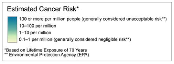
The magnitude of estimated cancer risk can be expressed in various ways. Lipkus summarized evidence on communicating probabilistic health risk,⁽³⁰⁾ noting people generally prefer numeric to verbal risk expressions,⁽³¹⁾ and natural frequencies are more easily and accurately understood than other numeric expressions.⁽³²⁾ Numeric relative risk expressions that lack a base rate are vague,⁽³⁰⁾ e.g., 10% more risk. The inclusion of base rates or other normative indicators support decision-making.⁽³³⁾ Verbal risk expressions are less precise, more intuitively understood,⁽³⁴⁾ influenced more by prior beliefs,⁽³⁵⁾ and generate less accurate perceptions than numeric expressions.⁽³⁶⁾ NATA maps⁽¹⁾ express cancer risk using natural frequencies (cancer cases per million people). Imprecise expressions of “Less” to “More” increase uncertainty because they verbally convey relative risk with no base rates or other normative indicators.

Safety standards and benchmarks are normative indicators that identify the safety meaning of risk levels.⁽³⁷⁾ Although the EPA applies multiple criteria to establish health standards, it strives for unofficial benchmarks of “negligible” risk no greater than 1 cancer case per million people and generally considers risk over 100 cancer cases per million as “unacceptable”.⁽³⁸⁾ Safety standards and benchmarks influence risk beliefs. Some studies show a sharp discontinuity in beliefs derived from amounts just above and below a standard rather than more appropriate dose-response interpretations,^{(29, 39, 40)} although this effect is not seen in other studies.⁽⁴¹⁾

1.1.2. Cognitive and Emotional Representations

Although knowledge is important, beliefs are more predictive of health behavior.^{(42, 43)} Among health behavior theories, the Common Sense Model (CSM) conceptualizes cognitive representations as comprised of structured risk beliefs.⁽⁴²⁾ Beliefs that identify the presence of a risk and one’s susceptibility to that risk have key roles in promoting protective risk behavior.^{(42, 44)} Specific beliefs underlying global beliefs include susceptibility to the risk, the severity of consequences,⁽⁴⁴⁾ and beliefs of exposure to unsafe hazard levels which will likely engender beliefs of susceptibility to consequential health problems. Learning and memory research guided by fuzzy trace theory indicates people seek to understand, and use for decisions, the basic gist of information rather than verbatim details.^{(45, 46)} Beliefs are a type of gist.

The CSM also recognizes the role of emotion in making decisions about health threats, and posits duel processing of cognitive and experiential information as shaping cognitive and emotional representations that shape behavior. CSM researchers relate this dual processing system to top-down and bottom-up processes.⁽⁴²⁾ Similarly, Loewenstein et al.⁽⁴⁷⁾ and Slovic et al.⁽⁴⁸⁾ describe the tendency for people to have positive and negative feelings about risk information and experience that shape decisions. Emotions vary in strength. Subtle feelings are described as affect, the “faint whisper of emotion” (p. 312).⁽⁴⁸⁾ Rivers et al. equate affect with emotional valence. Derived gist includes emotional valence.⁽⁴⁹⁾ The risk beliefs described here (e.g., serious problem, severe health consequence) have a negative valence. All of these perspectives recognize the powerful roles of experience in shaping emotions and emotional valence, and of emotion in shaping beliefs (gist) and decisions.^{(42, 47–50)}

Perceived ambiguity, generally interpreted as “uncertainty about uncertainty,” is generated when information is unreliable, incomplete, conflicting, or when expert knowledge is contested.⁽⁹⁾ People have an aversion to ambiguity, preferring certain over uncertain risks.⁽⁵¹⁾ This may explain why ambiguity often positively relates to perceived risk and worry.^{(9, 51–54)} Some studies show ambiguity attenuates heath behavior, while others do not.⁽⁹⁾

1.1.3. Personal Characteristics

Personal characteristics such as prior knowledge, prior beliefs, and prior experiences have substantial influences on how visual images,⁽⁵⁵⁾ including maps,⁽⁵⁶⁾ are understood. Unfavorable sensory perceptions of the environment, such as smell and appearance of outdoor air, increase perceived risk from air pollution.^{(57, 58)} One’s prior beliefs about air pollution risk may include skepticism about related health risks. People tend to be more skeptical of information that does not match tightly held beliefs, a type of bias that can influence how information is processed.⁽⁵⁹⁾ A family history of cancer is likely to increase risk beliefs generated by modeled cancer risk, especially since cancer is a dreaded disease.⁽⁶⁰⁾

Numeracy has been defined as “the ability to comprehend, use and attach meaning to numbers” (p. 262).⁽⁶¹⁾ Research indicates numeracy is a distinct construct from other indicators of cognition such as education, verbal intelligence, and health literacy.⁽⁶¹⁾ An experiment that examined responses to risk information found stronger perceived numeracy was related to weaker (and ultimately more accurate) risk beliefs.⁽⁶²⁾ In addition, low numeracy tends to foster affective responses to risk.⁽⁶³⁾

Research indicates sex has no influence on ambiguity related to cancer risk,⁽⁶⁴⁾ but females generally have stronger risk beliefs.⁽⁶⁵⁾ Females also tend to notice and recall visual details more than males, while males tend to see general trends more than females.⁽⁶⁶⁾

1.2. Purpose and Hypotheses

The purpose of this study was to assess how the “certainty” of three map features (contour focus, number of colors, risk expression) influenced risk beliefs and perceived ambiguity of risk beliefs for maps displaying four levels of modeled cancer risk. These influences were assessed within a context of personal characteristics. We propose: (a) focused contours, three colors, and numerically expressed risk convey more certainty than their counterparts of unfocused contours, one color, and verbally and relatively expressed risk; (b) these features will interact with lower and higher risk levels to influence risk beliefs such that certain features will be related to weaker risk beliefs for lower risk levels and stronger risk beliefs for higher levels; and (c) a positive dose-response relationship between risk level and the strength of risk beliefs.

Specific hypotheses (H) and research questions (RQ) include:

• H1. For all risk levels, less certain map features will generate more ambiguity.

• H2. For higher risk levels, more certain map features will generate stronger beliefs.

• H3. For lower risk levels, more certain map features will generate weaker beliefs.

• H4. For all risk levels, risk level will positively relate to the strength of risk beliefs.

• RQ 1. What is the influence of personal characteristics on risk beliefs and ambiguity?

• RQ 2. Do map variables (features, risk level) interact to influence risk beliefs and ambiguity?

• RQ 3. Do map features interact with personal characteristics to influence risk beliefs and ambiguity?

2. METHODS

2.1. Cancer Risk Model

The cancer risk maps used in this study were created from computer-based dispersion modeling analysis of estimated emissions from stationary and on-road air pollution sources. For stationary sources, the Wisconsin Department of Natural Resources annual emissions inventory provided the emissions inputs for the EPA Regional Air Impact Modeling Initiative (RAIMI) risk screening model. The RAIMI modeling system is a powerful GIS-based cumulative risk model that automates dispersion modeling over large areas by linking emissions inventory databases with the EPA Industrial Source Complex model (ISCST3).⁽⁶⁷⁾ The ISCST3 employs a Gaussian plume model to estimate air pollutant concentrations and resultant risks from multiple sources and pollutants. For mobile sources, estimates of on-road emissions were developed using roadway data in conjunction with the EPA MOBILE version 6.2 emissions model.⁽⁶⁸⁾ The resultant concentrations of pollutants were estimated using the AERMOD Gaussian plume dispersion model.⁽⁶⁹⁾ Roadway dispersion modeling was characterized as points representing vehicles (cars or trucks) and included a downwash algorithm. Cumulative cancer risk was derived by summing the pollutant concentrations and cancer risks for each type of source (stationary and on-road) and each pollutant at every receptor across the county.

Notably, maps represent computer-based estimations calculated from estimated annual concentrations of air pollutants rather than actual monitored pollutant levels. Given the uncertainty of this information, intended use is for identifying and prioritizing geographic areas and pollutants for further agency-level evaluation; not for appraising personal cancer risk.⁽⁷⁰⁾

2.2. Study Design, Map Variables, and Study Maps

This randomized experiment (no control group) assessed the influence of three map features hypothesized to convey more or less certainty about modeled cancer risk. This influence was assessed at four assigned map locations that varied by the four risk levels depicted in classed maps. Map features were (less certain vs. more certain): contour focus (unfocused vs. focused), color (1 color vs. 3 colors), and the risk expression used in the legend (verbal-relative) with no safety benchmarks vs. numeric natural frequencies with safety benchmarks). Independent map variables (IV) for this 2 × 2 × 2 × 4 factorial design are: contour focus, color, risk expression, and risk level. H2 and H3 propose differential effects for two subgroups: lower risk levels (risk levels of 1 and 2) and higher risk levels (risk levels of 3 and 4).

Eight maps were designed to vary by the three map features. Four versions were produced for each by adding a “You live here” location within one of the four risk level areas. The 32 study maps were arranged into eight blocks. Each block had two focused (F) and two unfocused (U) maps with risk levels of 1 and 3 (ordered U3, F1, F3, U1) or 2 and 4 (ordered U4, F2, F4, U2). Within blocks, maps did not vary by color or risk expression. Four representative blocks are available at http://research.son.wisc.edu/pollutionstudy/mapblocks.pdf. To control for ordering effects, maps were provided in reverse order in eight additional blocks.

Figure 2a depicts focused contours for a three color map. Figure 2b depicts unfocused contours for a one color map. Maps used sequential color schemes with incrementally darker shades to depict incremental risk. Each shows the four assigned map locations (risk levels 1–4) but study maps depicted one location per map.

Data classification produced focused or unfocused contours. For focused contours (Figure 2a), data was classified using four equal interval classes³ that spanned one power of ten as in NATA maps⁽⁷¹⁾ (Figure 2c). To control for the spatial distribution of modeled risk and decrease outlier influence, the unfocused “unclassed map” (Figure 2b) was actually a 32 class map with eight equal interval classes within each of the four classes.

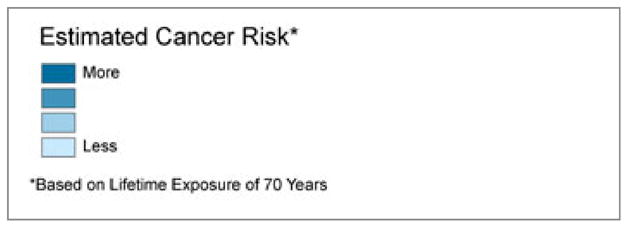
Legends were paired with either a numeric or verbal-relative risk expression. The numeric risk expression conveyed risk as the number of cancer cases per million and included safety benchmarks of “generally considered unacceptable risk” at risk level 4 and “generally considered negligible risk” at risk level 1 citing the “Environmental Protection Agency (EPA)” in a legend footnote (Figure 2c). The verbal-relative risk expression used only verbal relative risk terms of “Less risk” at risk level 1 and “More risk” at risk level 4 (Figures 2d). All map legends (eight versions) were labeled “Estimated Cancer Risk” and included this footnote “Based on lifetime exposure of 70 years.”

Maps depicted modeled cancer risk for Dane County, Wisconsin. The only landmarks were state and interstate highways with road labels and the outline of four major lakes at the map’s center. The largest lake was labeled and is a central feature of Madison (largest city in county) and of the University of Wisconsin (UW)-Madison from which the sample was drawn. Maps included a north arrow, scale, and inset showing the county’s location within Wisconsin.

Dane County, about 500,000 residents,⁽⁷²⁾ is a mix of rural and urban land uses and not highly industrialized. Madison and Dane County meet federal air quality standards with most days showing “good” quality.⁽⁷³⁾ We selected Dane county because data was readily available and showed geographic variability in cancer risk.

2.3. Survey Instrument and Study Sample

Dependent variables (DV) measured risk beliefs, emotion, and perceived ambiguity of risk beliefs (Appendix). Ten survey items assessed specific and global risk beliefs that identify risk at personal and neighborhood levels. Specific beliefs were exposure, susceptibility, and severity items. Global risk beliefs included perceived air safety and problem seriousness. One survey item, distress about air pollution risk, assessed discreet emotion. Most items had 6-point ordinal scales from strongly disagree to strongly agree. Two items had 11-point numeric scales. For each belief item, an ambiguity version was created by adding the phrase “It is hard to know” in front of the item, adapted from Han, Moser, and Klein.⁽⁹⁾ The ambiguity item directly followed the matching belief item. After these survey items, participants were asked to “briefly describe what the map tells you”. Participants first assessed an unfocused and then a focused map.

We used five items to control for and examine the influence of pre-map prior beliefs about outdoor air pollution for participants’ current residential location: sensory perceptions for smell and appearance, safety, prior ambiguity about air safety, and skepticism about air-pollution related health risks. As UW-Madison undergraduates, participants likely resided in the city of Madison or in Dane County; which were depicted on study maps. Given the assigned map locations, these items provided partial control. After maps, numeracy was assessed using the eight item subjective numeracy scale⁽⁷⁴⁾ that is strongly correlated with, but more user friendly than, objective measures of numeracy.⁽⁷⁵⁾ We also assessed gender, immediate family cancer diagnosis, and major area of study (Appendix).

About 1800 undergraduate students in eight classes at UW-Madison were invited to participate via a course website in the Psychology Department or by verbal invitations to students in three nursing classes. At the online survey website, students were randomly assigned to one of 16 map blocks. They answered risk belief, emotion, and ambiguity survey items as they viewed each map. It is unlikely that participants received information about Dane County air quality prior to the study.

2.4. Data Analysis

Exploratory factor analysis (EFA) with maximum likelihood (ML) estimation and promax rotation (PAWS Version 18),⁽⁷⁶⁾ followed by confirmatory factor analysis (CFA) (M-plus Version 5.1)⁽⁷⁷⁾ was used to create latent variables measuring prior risk beliefs, numeracy, risk beliefs, and ambiguity.

For H1-4 and RQ1-3, structural equation modeling (SEM) was used to assess the influences of personal characteristics and map variables on risk beliefs and ambiguity. CFA and SEM clustered participants to account for interdependence since each viewed four maps, and therefore used MLR⁴ estimation. Depending on the analysis, SEM was conducted for: (a) the total sample, (b) two subgroups: higher risk levels (risk level = 3, 4) and lower risk levels (risk level = 1, 2); or (c) four subgroups (risk levels 1–4). For subgroups, we used multi-group SEM with no paths constrained to be equal across subgroups. Analysis details are footnoted.⁵

3. RESULTS

826 students participated in the study that ended mid-semester, so a response rate could not be estimated. Chi-square tests showed no significant differences in categorical participant characteristics across the 4 risk levels: 66.3% were female (χ² = 0.01, p = 1.0); 32.9% reported a cancer diagnosis in their family (χ² = 3.36, p = 0.34); and 44% were in a health-related major, 1% environmental studies, and 55% another major or undecided. Health and environmental majors were merged (other, health) (χ² = 0.67, p = 0.88). ANOVA with posthoc comparisons (Sidak corrections) showed no differences in prior beliefs across the 4 risk level subgroups (results available from first author): means indicated prior beliefs of safe air [2.28(0.76]; slight disagreement for prior skepticism about air pollution-related health risks [2.9(1.06)]; and slight prior ambiguity about air safety [4.05(1.09)] (6-point scales).

3.1. Factor Analysis

EFA for prior beliefs prompted removing two low loading variables (< .32⁽⁷⁸⁾) resulting in a single factor that explained 48.6% of variance. Removed items (prior ambiguity about air safety and prior skepticism) were specified in the SEM as univariate observed variables. EFA identified two factors for numeracy (numeric ability and numeric preference) that explained 54.6% of variance. EFA among dependent risk belief and ambiguity variables resulted in 2 factors, risk beliefs and ambiguity that explained 68.9% of the variance among these 21 variables. The risk beliefs factor included all specific and global risk beliefs and emotion. The ambiguity factor included all ambiguity variables. Modification indices from CFAs of IVs and DVs prompted the addition of six correlated error terms to improve model fit.⁶ The highest loading on risk beliefs was exposure to air pollution and lowest was severity. Multi-group CFA was also conducted across the 4 risk levels.⁷ Standardized CFA loadings for all levels and across the four levels are available at http://research.son.wisc.edu/pollutionstudy/loadings.pdf.

Table I provides means and standard deviations across the four risk levels for the highest loading risk belief (exposure at a personal level) and companion ambiguity item. For beliefs, post hoc comparisons (ANOVA) indicated the largest mean difference was between risk levels 2 and 3. Ambiguity was larger for risk level 2 than 1, and for 3 than 4. Eta² indicated a linear relationship between risk level and risk beliefs, but not ambiguity.

Table I.

Mean Beliefs of Exposure to Unsafe Amounts of Air Pollution and Ambiguity of Beliefs at Four Risk Levels with Post-hoc ANOVA Comparisons¹ for Mean Differences between Risk Levels

	Mean and SD at Four Risk Levels (RL)				Eta2
	RL = 1	RL = 2	RL = 3	RL = 4
	n=814	n=804	n=818	n=800
Belief (exposed - me)	2.38	2.74	4.09	4.35	.36***
	1.08	1.05	1.11	1.13
Mean differences1 between levels (1,2) (2,3) (3,4)		−0.35***	−1.35***	−0.23***
Ambiguity (exposed - me)	3.24	3.45	3.59	3.44	.01
	1.30	1.20	1.23	1.28
Mean differences1 between levels (1,2) (2,3) (3,4)		−0.22**	−0.14	.15+

¹Sidak corrections for multiple tests

p < .10⁺,

p < .05*,

p < .01**,

p < .001***

Table II provides correlations among personal characteristics. The correlation between numeric ability and preference was large; most others were small or null. Stronger numeric ability and preference were related to male sex and viewing maps with a verbal-relative risk expression (numeracy was assessed after maps were viewed). Stronger prior risk beliefs were related to more prior ambiguity, female gender, weaker prior skepticism about health risks, less perceived numeric ability, and a health major. Stronger prior ambiguity was related to stronger prior risk beliefs, female gender, and less perceived numeric ability. Prior skepticism about air pollution-related health risks was related to a non-health major, male gender, and more numeric ability. Females were more likely to report being in a health major.

Table II.

Correlations Among User Characteristics:¹ All Risk Levels (n = 3270 observations)

	1	2	3	4	5	6	7	8
1. Prior beliefs	-
2. Prior ambiguity	.27***	-
3. Prior skepticism	−.15***	.01	-
4. Numerical ability	−.15**	−.09*	.10*	-
5. Numerical preference	−.09+	−.06	.03	.57***	-
6. Family cancer experience	.02	.02	−.01	.02	.04	-
7. Major (other, health)	.11**	.06	−.16***	.02	.06	.06	-
8. Sex	.18***	.15***	−.15***	−.28***	−.16***	.05	.28***	-
9. Risk expression1	−.02	−.03	0	−.08*	−.08*	.05	.01	0

¹We also included risk expression because it was the only map variable correlated with a user characteristic. Numerical ability and preference were assessed after participants viewed maps so may have been influenced by the risk expression.

p < .10⁺,

p < .05*,

p < .01**,

p < .001***

3.2. Map Variables on Beliefs and Ambiguity

Table III provides standardized SEM coefficients for the influence of map variables on ambiguity and risk beliefs across higher, lower, and all risk levels. Multicollinearity between numeric ability and preference prompted analyzing separate models for each. Table III provides coefficients for the model with numeric preference and the numeric ability variable. Coefficients for the model with numeric ability are at: http://research.son.wisc.edu/pollutionstudy/ability.pdf.

Table III.

Influence of Map Variables on Risk Beliefs and Ambiguity for Higher and Lower Risk Subgroups¹ and for All Risk Levels²: Standardized SEM Coefficients

Independent Variables		Standardized SEM Coefficients and R2
		Risk Beliefs			Ambiguity
		Higher Risk Levels (3, 4)	Lower Risk Levels (1, 2)	All Risk Levels (1–4)	Higher Risk Levels (3, 4)	Lower Risk Levels (1, 2)	All Risk Levels (1–4)
Explained Variance for DV	R2	.29	.21	.51	.13	.12	.11
Personal Characteristics
Numerical ability3 (provided for comparison)	γ	−.01	−.14***	−.05+	−.02	−.05	−.03
Numerical preference	γ	.07+	−.17***	−.03	−.08*	−.11**	−.09**
Prior beliefs	γ	.28***	.31***	.23**	−.18***	−.07	−.12**
Prior ambiguity	γ	.06+	−.11**	−.01	.23***	.21***	.22***
Prior skepticism	γ	−.16***	−.04	−.07***	.07+	.02	.05
Family cancer experience	γ	.14*	.04	.08*	−.14*	−.05	−.09
Major (other, health)	γ	.17**	.03	.08*	−.04	−.03	−.04
Sex	γ	.37***	.06	.17***	.05	.11	.08
Map Variables
Color	γ	.17***	.03	.07*	−.05	−.05	−.05
Contour focus	γ	.25***	−.24***	.01	−.15***	−.22***	−.18***
Risk expression	γ	−.02	−.23***	−.08*	−.34***	−.33***	−.33***
Risk level	γ	.34***	.39***	.58***	−.16*	.16**	.05

¹Fit Indices for multi-group risk model (high and low) is: SRMR = .047, RMSEA = .043, CFI = .909; n=1635 observations for higher and lower risk subgroups and n=3270 observations for all risk levels.

²Fit Indices for all risk levels model is: SRMR = .031, RMSEA = .035, CFI = .934

³The model with numerical ability had these R² values: R² = .281, .199 for beliefs (lower and higher risk levels); R² = .120, .105 for perceived ambiguity (lower and higher risk subgroups); R² = .511, .101 for beliefs and ambiguity (all risk levels).

p < .10⁺,

p < .05*,

p < .01**,

p < .001***

Figures 3 and 4 illustrate standardized SEM coefficients for the influence of personal characteristics and map features on ambiguity and risk beliefs at each risk level (H1 and H2). The Fig. 3 caption provides interpretive details. Fig. 5 illustrates significant interaction effects (RQ2 and RQ3).

Fig. 3.

illustrates the influence of map features and personal characteristics on ambiguity for risk levels 1–4. Incrementally darker shades of gray indicate incrementally larger risk levels. Bars represent standardized SEM coefficients significant at p < .05 or higher. Textured bars are non-significant. A longer bar indicates a stronger influence regardless of direction above or below the x-axis. Horizontal labels at the top and bottom indicate personal characteristics and map features related to stronger outcomes. Bars above the axis indicate personal characteristics, female gender, health major, and certain map variables related to stronger outcomes (positive coefficient); bars below indicate counterparts related to stronger outcomes (negative coefficient).

*Exp = Experience, Pref = Preference (note to type-setter – this should appear under Fig. 3

Fig. 4.

illustrates the influence of map features and personal characteristics on beliefs for risk 1–4. See the Fig.3 caption for interpretive details.

*Exp = Experience, Pref = Preference (note to type-setter – this should appear under Fig. 4

Fig. 5.

illustrates significant interaction effects (see x-axis) on risk beliefs (bars with black outlines) and ambiguity (no outlines) for RQ2 and RQ3. Bars show the SEM coeffient for the influence of the 1^st variable in the interaction term. See explanatory text for details.

a. RL = risk level, RE = risk expression, CF = contour focus, Co = color, Sk = skepticism, Np = numerical preference

b. ns = not significant (all others are significant at p < .05)

(note to type-setter – a. and b. should appear under Fig. 5)

3.2.1. Ambiguity

RQ1. Influence of personal characteristics

For all risk levels (Table III), more prior ambiguity and less preference for numeric information fostered more ambiguity. For higher risk levels, weaker prior beliefs and less cancer experience fostered more ambiguity.

H1. For all risk levels, less certain map features will generate more ambiguity

H1 was supported for contour focus (unfocused generated more ambiguity than focused) and risk expression (verbal-relative generated more ambiguity than numeric), but not for color (Table III, Fig. 3).

RQ2. Interactions among map variables

At lower risk levels, interactions indicated (see Fig. 5): risk level generated more ambiguity for focused than unfocused contours: (.09, p = .08; #4); and unfocused contours generated more ambiguity for the numeric than verbal-relative risk expression (.07, p < .01, #7) and for maps with 1 than 3 colors (.05, p = .08; #6). Only the last interaction fully supports H1.

3.2.2. Risk beliefs

RQ1. Influence of personal characteristics

Stronger prior beliefs of poor air fostered stronger risk beliefs for all risk levels (Table III, Fig. 4). For higher risk levels (Table III), female sex, a health major, less prior skepticism, and family cancer experience were related to stronger risk beliefs. For lower risk levels (Table III), weaker numeric preference and ability, and less prior ambiguity were related to stronger beliefs.

H2. For higher risk levels, more certain map features will generate stronger beliefs

This hypothesis was supported for contour focus (focused generated stronger beliefs) and color (three colors generated stronger beliefs) but not for risk expression (Table III). Fig. 4 suggests null findings for risk expression occurred due to the positive effect (but null) of risk expression on beliefs at risk level 4 but negative effect at level 3 (verbal-relative risk fostered stronger beliefs).

RQ2. Interactions among map variables – higher risk levels

The interaction effect between risk level and risk expression was marginally significant (.35, p = .09). Fig. 5 (interaction #1) illustrates that risk level generated somewhat stronger risk beliefs for the numeric than the verbal-relative risk expression. An interaction effect between risk level and contour focus (.41, p < .001; Fig. 5, #2) indicates risk level generated stronger beliefs for focused than unfocused contours. These interaction effects further support H2; risk level had a stronger effect for certain compared to uncertain map features.

H3. For lower risk levels, more certain map features will generate weaker beliefs

This hypothesis was supported for contour focus (focused generated weaker beliefs) and risk expression (numeric generated weaker beliefs), but not for color (Table III, Fig. 4).

RQ2. Interactions among map variables – lower risk levels

An interaction between risk level and contour focus occurred because risk level generated stronger beliefs for focused than unfocused contours (.15, p < .01; Fig. 5, #3). An interaction between color and contour occurred because unfocused contours generated stronger beliefs for 1 color than 3 (.07, p < .05; Fig 5, #5).

H4. For all risk levels, risk level will positively relate to the strength of risk beliefs

H4 was fully supported. Risk level had a large influence on risk beliefs (moderate influence for higher and lower risk subgroups) (Table III). Across subgroups, risk level had a small positive influence on ambiguity for lower risk levels and small negative effect for higher risk, reflecting the mean ambiguity differences in Table I.

Correlations between risk beliefs and ambiguity varied by risk level (Fig. 6). At lower risk levels, stronger risk beliefs were related to more ambiguity. At higher risk levels, stronger risk beliefs were related to less ambiguity.

Fig. 6.

3.2.3. RQ3. Interactions between Map Variables and Personal Characteristics

Interactions were only between risk expression and numeric preference or prior skepticism. Less numeric preference or prior skepticism generated stronger risk beliefs or ambiguity more for the numeric than the verbal-relative risk expression (Fig. 5). Results are: risk expression*skepticism on risk beliefs (higher risk) = .24, p < .05 (#8); risk expression*numeric preference on risk beliefs (lower risk) = .26, p < .05 (#9); risk expression*numeric preference on ambiguity (higher risk) = .22, p < .05 (#10) and (lower risk) = .31, p < .001 (#11).

4. DISCUSSION

4.1. Map Features and Risk Level on Risk Beliefs and Ambiguity

4.1.1. Risk Level

Risk level had the most dominant influence on how participants identified personal- and neighborhood-level risk, suggesting that shaded isarithmic maps can effectively communicate dose-response relationships for geographic risk information. Bottom-up comprehension of pre-attentive incremental color shading surrounding (proximal to) assigned map locations in tandem with top-down processing to answer questions about risk for assigned map locations likely enhanced risk level’s influence. The iconic resemblance of shading to communicate increasing magnitude and of assigned map location to communicate participants’ proximity to risk further supports comprehension. The vertically ordered legend categories may have enhanced the dose-response meaning derived from the map due to bottom-up processing of pre-attentive position on a scale⁽¹³⁾ (incremental legend categories) and direction⁽¹³⁾ from low to high. Others have found that vertical orientation relates to increasing magnitude.⁽⁷⁹⁾

4.1.2. Contour Focus

Data classification produces focused (classed) or unfocused (unclassed) map contours. Contours were the unit of perception, a key factor proposed to shape what people see and derived bottom-up meaning.⁽¹²⁾ The substantial influence of contour focus on ambiguity and risk beliefs supports this proposition as did an earlier study of a different mapped hazard and perceptual units.⁽³⁾ The iconic visual appearance of “in focus” or “out of focus” to convey a gist of certainty or uncertainty explains results showing full support for the hypothesized influence of contour focus on ambiguity. For unfocused maps, the lack of discrete incremental risk levels in the map and legend, and related top-down difficulty of matching map and legend colors add to perceptual unit’s influence. This study participant’s comment illustrates these explanations; “The gradual shading made it more difficult to decide where exactly each spot fell on the spectrum of cancer risk.” Conveying uncertainty, such as modeled cancer risk, is a risk communication challenge.⁽⁸⁰⁾ Depicting uncertain information as out of focus shows promise for addressing that challenge.

Full support for the hypothesized influence of focused contours to generate stronger beliefs for higher risk levels and weaker beliefs for lower risk levels is explained by bottom-up comprehension of incremental risk due to the discreet and incrementally shaded risk levels in the map and legend, and the top-down ease of matching map and legend colors. This participant’s comment illustrates the advantage of classed maps; “the lines are more clear-cut so you can easily tell what areas have which levels of air pollution.” Findings and quotes support MacEachren’s proposition that contour focus effectively represents the certainty of information.⁽⁴⁾ More broadly, iconic representations may be effective for conveying certainty.

Results illustrate that location-based risk level (essentially proximity to mapped risk) has a larger influence on participants’ ability to identify person- and neighborhood-level risk for focused than unfocused maps. We conclude that perceptual unit interacts with risk level to influence beliefs such that visually distinct units depicting defined areas of risk amplify the impact of shaded risk level compared to fuzzy unfocused units. Assigned participant locations that were well within the defined risk areas likely strengthened these interaction effects.

Notably, contour focus is a by-product of producing classed and unclassed maps. An unfocused unclassed map is a more accurate representation of the risk data than a focused classed map.⁽¹⁴⁾ Other methods of visualizing uncertainty^{(4, 7, 8, 23)} require intrinsic modifications to the appearance of map features, or the extrinsic addition of uncertainty features to a map.

4.1.3. Risk Expression

As predicted, the less certain verbal-relative risk expression generated ambiguity at all risk levels. The substantial influence of risk expression on ambiguity is indicated by this participant’s comment about the relative nature of the verbal-relative risk expression; “the map provides a non-scaled risk of harm, pretty ambiguous.” This participant’s comment indicates the absence of base rates generates ambiguity “…because it [verbal-relative risk expression] could have been from 0% – 100% or 1% –3%; whether I would have felt unsafe if I lived in a region with ‘more’ risk would have varied greatly depending on whether ‘more’ meant 100% or 3%.” Comments suggest the lack of a normative base rate had a greater influence on ambiguity than the verbal nature of the risk expression.

For risk levels 1–3, the numeric risk expression may have provided a less threatening message for four reasons. First, the ambiguity of the verbal-relative risk expression tends to heighten perceived risk and associated emotion compared to less ambiguous numeric risk.^{(9, 53, 54, 81)} Second, initial numbers in the numeric range were small (0.1, 1, 10), and likely perceived as smaller if compared to the denominator of a million people. Third, these small numbers were on the leading left edge of the range, thus likely more visually salient than the larger numbers on the right edge. Fourth, some studies show people attend more to the frequency of harm, small in this case, than the population at risk.⁽⁸²⁾ Collectively, these explain why the numeric expression prompted weaker beliefs at risk levels 1–3; supporting our hypothesis for lower but not higher risk levels.

The “unacceptable” benchmark at risk level 4 in the numeric risk expression may explain why participants had a non-significant trend of stronger beliefs at level 4 for the numeric expression, but stronger beliefs at level 3 for the verbal-relative expression. This is consistent with findings of discontinuity effects for beliefs generated by risk levels just below or above a safety indicator.⁽⁴⁰⁾ The personal relevance of the benchmark for students in a health major may explain their stronger risk beliefs at level 4. Finally, using interpolation to derive meaning for the unlabeled risk levels in the verbal-relative expression (levels 2, 3) may have generated additional ambiguity.

Interaction effects indicated numeric preference and skepticism moderated the main effects of risk expression. At lower and higher risk levels, less comprehension of numeric relationships may have generated more ambiguity for the numeric expression; supported by this participant’s comment, “The thing that is confusing about this map is the ratios they give in the key.” Aversion to ambiguity⁽⁵¹⁾ may have prompted some participants assigned to the verbal-relative expression to indicate a numeric preference (Table II).

The scientific appearance of, and use of “people” in, the numeric expression may convey a gist of credibility and seriousness. For lower risk levels and participants with less numeric preference, the gist of credibility and seriousness together with decreased comprehension of the smaller numbers and probabilities may have generated stronger beliefs, feelings, and ambiguity compared to the easily comprehended verbal-relative expression of “Less”. For higher risk levels, less prior skepticism (bias) about air pollution-related health effects may have allowed participants to adopt stronger beliefs, and more so for the numeric expression due to the gist of credibility and seriousness.

Notably, numeracy only influenced outcomes for the numeric risk expression, likely due to its alphanumeric content. An absence of numbers explains why numeric preference had no effects for the verbal-relative expression. In addition, contour focus and incremental shading operated similarly across participants who varied in perceived numeracy indicating these visual features addressed numeracy barriers for communicating information uncertainty and incremental risk. Although a distinct construct,⁽⁶¹⁾ numeracy is viewed as a component of health and science literacy,⁽⁸³⁾ and all are relevant to environmental health. Results suggest visual map features may go beyond numeracy to address other aspects of health and science literacy.

Unfocused contours generated more ambiguity for the numeric than the verbal-relative risk expression (Fig. 5, #7). When the legend has numeric risk levels, participants may be motivated to match their map location color to the legend to determine numeric risk. Inability to accurately match unfocused graded colors to the numeric legend scale may increase perceived ambiguity. Since incremental shading pre-attentively and iconically conveys “Less” to “More,” the verbal-relative risk expression in the legend is redundant; therefore matching a map location’s color to the legend is less meaningful. Fewer attempts to match map locations to the verbal-relative risk expression may decrease ambiguity compared to the numeric risk expression. Those creating maps should consider how features work together to communicate a coherent message.

4.1.4. Number of Colors

We expected more than the weak interaction effects found between color and contour focus because additional colors should enhance the matching process substantially more for unfocused maps than those with only 4 classes, as fewer classes increase visual discrimination of a single shaded color.⁽²⁵⁾ The dominant pre-attentive and iconic influence of incrementally darker shading to convey incremental risk may have overshadowed the influence of additional colors on unfocused maps resulting in smaller interaction effects. In addition, stronger beliefs for unfocused blue than multicolor maps at lower risk levels may have occurred because at risk levels 1 and 2, blue appeared darker than yellow and light green.

4.1.5. Personal Characteristics

Map features exerted effects within a context of personal characteristics. Published evidence that prior risk beliefs have a substantial influence on knowledge and beliefs derived from images^{(55, 56)} supports our findings for the sizable effects of prior risk beliefs and ambiguity on outcomes. When expected and depicted air pollution risk is not aligned, weaker prior risk beliefs may generate ambiguity. When risk is low, numeracy, prior beliefs, and prior ambiguity may have a stronger influence on beliefs and feelings than gender. Finally, a lack of interaction effects between sex and map features does not support previous observations that sex moderates visual cognition.⁽⁶⁶⁾ Influences of numeric preference and skepticism were discussed earlier.

4.1.6. Emotion, Relationship between Risk Beliefs and Ambiguity

The integration of distress and beliefs (some with considerable emotional valence) into a single latent risk belief variable indicates emotion played a role in participants’ cognitive responses to the maps, consistent with findings on the role of emotion.^{(42, 47–49)} The distinction between cognitive and emotional responses cannot be discerned because risk beliefs included aspects of both.

Only results at lower risk levels support other’s conclusions that uncertainty relates to stronger risk beliefs.⁽⁵²⁾ Emotions generated by the ambiguity of lower risks and associated with low numeracy, described earlier and noted by others,^{(9, 51–54, 63)} could foster stronger beliefs. At higher risk levels, uncertainty was related to weaker beliefs. The strong bottom-up response to incrementally darker colors that iconically represented incremental magnitude may explain why participants were, appropriately, more ambiguous about stronger beliefs at lower risk levels and weaker beliefs at higher risk levels (Fig. 6). The larger gap in beliefs between risk levels 2 and 3 suggests place-based air pollution perceptions, lower for rural than urban,⁽⁵⁸⁾ moderates the influence of risk level on risk beliefs.

4.2. Limitations

Since there were no adjustments for assessing multiple interactions (some significant values expected due to chance), these exploratory results should be cautiously interpreted. The study design does not support examining the separate effects of risk expression components (verbal-numeric, relative-objective, safety benchmarks) because the numeric expression included benchmarks. The student sample hinders generalizing results to the public due to: homogeneity in age and education level, and less personal relevance for the fictitious “you live here” locations and for risk estimates based on 70 years of exposure. While earlier maps likely exerted a training effect for later maps, we reversed map order for half the sample, and accounted for map order and intra-individual dependencies in the analysis. Although we could not control for variance in map appearance across computers, this increases external validity for online risk maps.

4.3. Implications

4.3.1. Broad Implications

Identifying effective methods for conveying the uncertainty of mapped risk information is important because maps show promise as an effective tool for informing the public about the geographic distribution of environmental risk. Although websites often include written disclaimers on the limitations of and appropriate uses for available maps, methods are needed to convey the gist of uncertainty within maps because users are likely to skip the disclaimers and maps are likely to convey lasting meaning. Most encouraging are findings that ambiguity was stronger for less appropriate dose-response beliefs. Contour focus paired with incremental shading show promise for addressing numeracy barriers and fostering appropriate dose-response beliefs and levels of ambiguity. Numeric and verbal-relative risk expressions were also effective for conveying certainty, but the effectiveness of the numeric expression was compromised when numeracy was low. Such methods support sharing uncertain information with the public and related goals of increasing transparency regarding the work of agencies,^{(84, 85)} encouraging informed community action,⁽⁸⁶⁾ and public participation in policy decisions.⁽⁸⁷⁾

Studies provide mixed evidence for the influence of ambiguity on behavior,⁽⁹⁾ ambiguity can impede taking action.^{(9, 88)} However, given (a) the power of images to shape meaningful gist, (b) the effectiveness of darker color to communicate increasing risk, and (c) the negative valence of heightened risk beliefs, we posit that maps with or without uncertain features are more likely than text information to support decision-making and motivate action. For example, some may be motivated to advocate for better public transportation. Personal characteristics, especially prior risk beliefs, are likely to play a substantial role in explaining how maps motivate action.

4.3.2. Implications for Theory

The most powerful visual features, contour focus and shading, were conceptualized as having both bottom-up and iconic influences. We propose that iconicity operates on a continuum between two basic modes of resemblance. Icons can resemble features that are processed bottom-up and icons can resemble “real-world” meaning that is readily available from long-term memory, e.g., a tent to depict a campground or blue to denote bodies of water. For iconic signs that are processed bottom-up, the neurological link between vision and cognition supports comprehension. MacEachren noted other perspectives on iconicity⁽²²⁾ such as the mimetic to abstract continuum proposed by Robinson and others.^{(21, 89)} The bottom-up to real-world resemblance continuum complements these other perspectives.

4.3.3. Implications for Research

Results provide abundant suggestions for further study. Several factors may moderate how contour focus influences risk beliefs and ambiguity. More data classes may attenuate effects by decreasing the visual contrast between incremental risk levels on classed maps and by increasing visual complexity. For a given dataset, perceptual unit’s size will be influenced by the number of classes; the distinct influence of each variable should be examined. More colors may enhance visual contrast and mitigate the influence of the number of classes. A diverging color scheme (especially a spectral diverging scheme)^{(25, 26)} may decrease the influence of contour focus by further enhancing visual contrast across risk levels on unfocused unclassed maps. Symbolic risk colors (e.g., red conveys warning) may influence risk beliefs and ambiguity and exert more influence for larger than smaller units of perception. Including an alphanumeric control, measures that discriminate between cognition and emotion, and appropriate decisional outcomes would provide evidence on theoretical mechanisms that explain how images influence these dependent variables. Including health or science literacy measures would support exploring how map features address these barriers to cognition. Comparing maps that depict either total estimated cancer risk or total estimated carcinogenic air pollution would assess whether and how people discriminate between these two risk model endpoints; the former is more uncertain as it includes estimated cancer potencies. To establish external validity, studies are needed among representative samples and using participants’ perceived map locations for their actual residence because personal relevance influences interpretations of risk information⁽⁴⁴⁾ including mapped risk.⁽³⁾ Following participation, study participants should be informed about the uncertainty of modeled cancer risk and then debriefed to assure comprehension because the study information could generate unwarranted anxiety for some individuals.

4.3.4. Implications for Practice

Those creating maps of modeled risk for public audiences should consider how the uncertainty of this information can be embodied in map features. Unfocused unclassed (or many-classed) isarithmic maps of continuous data appear to be an effective method for conveying uncertainty; an attractive option because they depict data more accurately than classed maps. Incrementally darker shading was very effective for conveying incremental risk. The verbal-relative risk expression also resulted in substantially more ambiguous beliefs, but did not allow external comparisons to other risk levels or normative indicators; a potential limitation depending on communication goals. Uncertain features resulted in stronger beliefs at lower risk levels, another tradeoff to consider when creating maps for public audiences. Interaction effects suggest practitioners should consider how features work together to communicate a coherent message. Feedback from the target audience should inform the final selection of features.

5. Conclusions

Visual features addressed communication challenges of conveying information uncertainty and a dose-response message. The effectiveness of these features is explained by (a) the iconicity of contour focus and incrementally darker color shading to convey uncertainty and incremental risk for assigned map locations, and (b) bottom-up processing of unit of perception (contour focus) and pre-attentive features (shading). For unfocused contours, the ambiguity generated by the difficulty of matching map and legend colors explains how top-down processing to identify location-based risk contributed to bottom-up influences. The power of incremental shading to convey a dose-response message appropriately generated more certainty for beliefs that were aligned with risk levels. Additionally, risk level interacted with contour focus such that risk level had stronger effects on beliefs for focused perceptual units that illustrated discrete risk level increments and facilitated matching map and legend colors. The expected geographic distribution of risk level from rural to urban locations reinforced and modified the incremental risk message. The lack of normative base rates and safety benchmarks explains why the verbal-relative risk expression generated substantially more ambiguity than the numeric risk expression. Unlike the numeric risk expression, iconic and pre-attentive map features addressed numeracy barriers for communicating information uncertainty and incremental risk. Overall, results indicate incremental shading effectively conveys a dose-response message, and contour focus and risk expression show promise for conveying information uncertainty. Further research is needed to confirm and extend these findings.

References

- 1.U.S. Environmental Protection Agency. [Accessed on September 20, 2011];Summary Results for the 2005 National-Scale Assessment. 2011 Available from: http://www.epa.gov/ttn/atw/nata2005/05pdf/sum_results.pdf.
- 2.Wartenberg D. Some considerations for the communication of results of air pollution health effects tracking. Air Quality, Atmosphere, and Health. 2009;2:207–21. doi: 10.1007/s11869-009-0046-y. [DOI] [PMC free article] [PubMed] [Google Scholar]
- 3.Severtson DJ, Vatovec C. The theory-based influence of map features on risk beliefs: Self-reports of what is seen and understood for maps depicting an environmental health hazard. Journal of Health Communication: International Perspectives. 2012:1–21. doi: 10.1080/10810730.2011.650933. Online. [DOI] [PMC free article] [PubMed] [Google Scholar]
- 4.MacEachren AM. Visualizing uncertain information. Cartographic Perspective. 1992;13:10–9. [Google Scholar]
- 5.Bostrom A, Anselin L, Farris J. Visualizing seismic risk and uncertainty. A review of related research Annals of the New York. Academy of Sciences. 2008;1128(1):29–40. doi: 10.1196/annals.1399.005. [DOI] [PubMed] [Google Scholar]
- 6.Harrower M, editor. UCGIS Workshop: Geospatial Visualization and Knowledge Discovery Workshop. Landsdowne, VA: 2003. Representing uncertainty: Does it help people make better decisions? [Google Scholar]
- 7.MacEachren AM, Robinson A, Hopper S, Gardner S, Murray R, Gahegan M, Hetzler E. Visualizing geospatial information uncertainty: What we know and what we need to know. Cartography and Geographic Information. Science. 2005;32(3):139–60. [Google Scholar]
- 8.Pang AT, Wittenbrink CM, Lodha SK. Approaches to uncertainty visualization. The Visual Computer. 1997;13(8):370–90. [Google Scholar]
- 9.Han PKJ, Moser RP, Klein WMP. Perceived ambiguity about cancer prevention recommendations: Relationship to perceptions of cancer preventability, risk, and worry. Journal of Health Communication. 2006;11:51–69. doi: 10.1080/10810730600637541. [DOI] [PMC free article] [PubMed] [Google Scholar]
- 10.Kim M-S, Hunter JE. Relationships among attitudes, behavioral intentions, and behavior. Communication Research 1993. 1993 Jun 1;20(3):331–64. [Google Scholar]
- 11.Sheeran P. In: Intention-behavior relations: A conceptual and empircal review. Stroebe W, Hewstone M, editors. Wiley & Sons; 2002. pp. 1–36. [Google Scholar]
- 12.Pinker S. A theory of graph comprehension. In: Freedle R, editor. Artificial intelligence and the future of testing. Hillsdale, NJ: Lawrence Erlbaum Associates, Publishers; 1990. pp. 73–126. [Google Scholar]
- 13.Cleveland WS, McGill R. Graphical perception: Theory, experimentation, and application to the development of graphical methods. Journal of the American Statistical Association. 1984;79(387):531–54. 09. [Google Scholar]
- 14.Slocum TA, McMaster RB, Kessler FC, Howard HH. Thematic cartography and geographic visualization. 3. Upper Saddle River, NJ: Prentice Hall; 2009. [Google Scholar]
- 15.Harrower M. Unclassed animated choropleth maps. The Cartographic Journal. 2007;44(4):313–20. [Google Scholar]
- 16.Cromley RG. Classed versus unclassed maps: A question of how many classes. Cartographica. 1995;32(4):15–27. [Google Scholar]
- 17.Mersey JE. Color and thematic map design: The role of color scheme and map complexity in choropleth map communication, Monograph 41. Cartographica. 1990;27(3):1–167. [Google Scholar]
- 18.Gilmartin P, Shelton E. Choropleth maps on high resolution CRTs: The effects of number of classes and hue on communication. Cartographica. 1989;26(2):40–52. [Google Scholar]
- 19.Slocum TA, McMaster RB, Kessler FC, Howard HH. Thematic cartography and geographic visualization. 3. Upper Saddle River, NJ: Prentice Hall; 2009. Choropleth mapping; pp. 251–70. [Google Scholar]
- 20.Chandler D. Semiotics: The basics. London: Routledge; 2002. [Google Scholar]
- 21.Robinson AH, Sale RD, Morrison JL, Muehrcke PC. Elements of Cartography. New York: Wiley; 1984. [Google Scholar]
- 22.MacEachren AM. How maps work: Representation, visualization, and design. New York: The Guilford Press; 1995. A functional approach to map representation; pp. 244–309. Paperback ed. [Google Scholar]
- 23.Pang A. Visualizing uncertainty in geo-spatial data. 2001. [Google Scholar]
- 24.Howard D, MacEachren AM. Interface design for geographic databases: Tools for representing reliability. Cartography and Geographic Information Systems. 1996;23(2):59–77. [Google Scholar]
- 25.Brewer CA. Basic mapping principles for visualizing cancer data using geographic information systems (GIS) American Journal of Preventive Medicine. 2006;30(2 Supplement 1):S25–S36. doi: 10.1016/j.amepre.2005.09.007. [DOI] [PubMed] [Google Scholar]
- 26.Brewer CA, Harrower M, Woodruff A, Heyman D. ColorBrewer 2.0. Pennsylvania State University and Axix Maps LLC; 2009. [Accessed on September 15, 2011]. Available from: http://colorbrewer2.org/ [Google Scholar]
- 27.Severtson DJ. Research in Nursing & Health. Maps as risk communication: The influence of environmental hazard maps on risk beliefs, emotion and protective behavior. In review. [DOI] [PMC free article] [PubMed] [Google Scholar]
- 28.Severtson DJ, Burt JE. The influence of mapped hazards on risk beliefs: A proximity-based modeling approach. Risk Analysis. 2012;32(2):259– 80. doi: 10.1111/j.1539-6924.2011.01700.x. [DOI] [PMC free article] [PubMed] [Google Scholar]
- 29.Weinstein ND, Sandman PM. Some criteria for evaluating risk messages. Risk Analysis. 1993;13(1):103–14. [Google Scholar]
- 30.Lipkus IM. Numeric, verbal, and visual formats of conveying health risks: Suggested best practices and future recommendations. Medical Decision Making. 2007;27(5):696–713. doi: 10.1177/0272989X07307271. [DOI] [PubMed] [Google Scholar]
- 31.Wallsten T, Budescu D, Zwick R, Kemp S. Preferences and reasons for communicating probabilistic information in verbal or numerical terms. Bulletin of the Psychonomic Society. 1993;31:135–8. [Google Scholar]
- 32.Hoffrage U, Gigerenzer G, Krauss S, Martignon L. Representation facilitates reasoning: what natural frequencies are and what they are not. Cognition. 2002;84(3):343–52. doi: 10.1016/s0010-0277(02)00050-1. [DOI] [PubMed] [Google Scholar]
- 33.Koehler J. The base rate fallacy reconsidered: Descriptive, normative and methodological challenges. Behavioral and Brain Sciences. 1996;19(1):1–53. [Google Scholar]
- 34.Moxey LM, Sanford AJ. Communicating quantities: a review of psycholinguistic evidence of how expressions determine perspectives. Applied Cognitive Psychology. 2000;14(3):237–55. [Google Scholar]
- 35.Fox CR, Irwin JR. The role of context in the communication of uncertain beliefs. Basic & Applied Social Psychology. 1998;20(1):57–70. [Google Scholar]
- 36.Knapp P, Raynor DK, Berry DC. Comparison of two methods of presenting risk information to patients about the side effects of medicines. BMJ Quality & Safety. 2004;13(3):176–80. doi: 10.1136/qshc.2003.009076. [DOI] [PMC free article] [PubMed] [Google Scholar]
- 37.Weinstein ND, Sandman PM, Miller P. Report to US EPA from Environmental Communication Research Program. New Brunswick, NJ: Cook College, Rutgers University; 1991. Communicating effectively about risk magnitudes: Phase two. Report No.: EPA-230-09-91-003. [Google Scholar]
- 38.U.S. Environmental Protection Agency; Quality OoA. Residual risk report to congress. Research Triangle Park, NC: 1999. [Google Scholar]
- 39.Johnson BB. Communicating air quality information: Experimental evaluation of alternative formats. Risk Analysis. 2003;23(1):91–103. doi: 10.1111/1539-6924.00292. [DOI] [PubMed] [Google Scholar]
- 40.Weinstein ND, Sandman PM. Predicting homeowners’ mitigation responses to radon test data. Journal of Social Issues. 1992;48(4):63–83. [Google Scholar]
- 41.Johnson B. Public views on drinking water standards as risk indicators. Risk Analysis. 2008;28(6):1515–30. doi: 10.1111/j.1539-6924.2008.01116.x. [DOI] [PubMed] [Google Scholar]
- 42.Leventhal H, Brissette I, Leventhal E. The common-sense model of self-regulation of health and illness. In: Cameron LD, Leventhal H, editors. The self-regulation of health and illness behavior. London: Routledge; 2003. pp. 42–65. [Google Scholar]
- 43.National Cancer Institute. Theory at a glance: A guide for health promotion practice. 2. Washington D.C: National Institutes of Health; 2005. [Google Scholar]
- 44.Weinstein ND. The precaution adoption process. Health Psychology. 1988;7:355–86. doi: 10.1037//0278-6133.7.4.355. [DOI] [PubMed] [Google Scholar]
- 45.Reyna VF, Brainerd CJ. Fuzzy-trace theory: An interim synthesis. Learning and Individual Differences. 1995;7(1):1–75. [Google Scholar]
- 46.Reyna VF, Brainerd CJ. Fuzzy-trace theory: Some foundational issues. Learning and Individual Differences. 1995;7(2):145–62. [Google Scholar]
- 47.Loewenstein GF, Weber EU, Hsee CK, Welch N. Risk as feelings. Psychological Bulletin. 2001;127(2):267–86. doi: 10.1037/0033-2909.127.2.267. [DOI] [PubMed] [Google Scholar]
- 48.Slovic P, Finucane ML, Peters E, MacGregor DG. Risk as analysis and risk as feelings: Some thoughts about affect, reason, risk, and rationality. Risk Analysis. 2004;24(2):311–22. doi: 10.1111/j.0272-4332.2004.00433.x. [DOI] [PubMed] [Google Scholar]
- 49.Rivers SE, Reyna VF, Mills B. Risk Taking Under the Influence: A Fuzzy-Trace Theory of Emotion in Adolescence. Developmental Review. 2008;8(1):107–44. doi: 10.1016/j.dr.2007.11.002. [DOI] [PMC free article] [PubMed] [Google Scholar]
- 50.Weinstein ND. Effects of personal experience on self-protective behavior. Psychological Bulletin. 1989;105:31–50. doi: 10.1037/0033-2909.105.1.31. [DOI] [PubMed] [Google Scholar]
- 51.Camerer C, Weber M. Recent developments in modeling preferences: Uncertainty and ambiguity. Journal of Risk and Uncertainty. 1992;5:325–70. [Google Scholar]
- 52.Griffin R, Dunwoody S, Neuwirth K. Proposed model of the relationship of risk information seeking and processing to the development of preventive behaviors. Environmental Research. 1999;80(2 part 2):S230–S45. doi: 10.1006/enrs.1998.3940. [DOI] [PubMed] [Google Scholar]
- 53.Powell M, Dunwoody S, Griffin R, Neuwirth K. Exploring lay uncertainty about an environmental health risk. Public Understanding of Science. 2007 Jul 1;16(3):323–43. [Google Scholar]
- 54.Viscusi WK, Magat WA, Huber J. Communication of ambiguous risk information. Theory and Decision. 1991;31(2):159–73. [Google Scholar]
- 55.Cook MP. Visual representations in science education: The influence of prior knowledge and cognitive load theory on instructional design principles. Science Education. 2006;90(6):1073–91. [Google Scholar]
- 56.Verdi MP, Kulhavy RW. Learning with maps and text: An overview. Educational Psychology Review. 2002:27–46. [Google Scholar]
- 57.Bickerstaff K, Walker G. Public understandings of air pollution: the localisation of environmental risk. Global Environmental Change. 2001;11(2):133–45. [Google Scholar]
- 58.Brody SD, Peck BM, Highfield W. Examining localized patterns of air quality perception in Texas: A spatial and statistical analysis. Risk Analysis. 2004 Mar 1;24(6):1561–74. doi: 10.1111/j.0272-4332.2004.00550.x. [DOI] [PubMed] [Google Scholar]
- 59.Ditto PH, Lopez DF. Motivated skepticism: The use of differential decision criteria for preferred and non-preferred conclusions. Journal of Personality and Social Psychology. 1992;63:568–84. [Google Scholar]
- 60.Trumbo CW, McComas KA, Kannaovakun P. Cancer anxiety and the perception of risk in alarmed communities. Risk Analysis. 2007;27(2):337–50. doi: 10.1111/j.1539-6924.2007.00886.x. [DOI] [PubMed] [Google Scholar]
- 61.Nelson W, Reyna VF, Fagerlin A, Lipkus I, Peters E. Clinical implications of numeracy: Theory and practice. Annals of Behavioral Medicine. 2008;35:261–74. doi: 10.1007/s12160-008-9037-8. [DOI] [PMC free article] [PubMed] [Google Scholar]
- 62.Zikmund-Fisher BJ, Ubel PA, Smith DM, Derry HA, McClure JB, Stark A, Pitsch RK, Fagerlin A. Communicating side effect risks in a tamoxifen prophylaxis decision aid: The debiasing influence of pictographs. Patient Education and Counseling. 2008;73(2):209–14. doi: 10.1016/j.pec.2008.05.010. [DOI] [PMC free article] [PubMed] [Google Scholar]
- 63.Peters E, Hibbard J, Slovic P, Dieckmann N. Numeracy skill And the communication, comprehension, and use of risk-benefit information. Health Affaies. 2007;26(3):741–8. doi: 10.1377/hlthaff.26.3.741. [DOI] [PubMed] [Google Scholar]
- 64.Han PKJ, Moser RP, Klein WMP, Beckjord EB, Dunlavy AC, Hesse BW. Predictors of perceived ambiguity about cancer prevention recommendations: Sociodemographic factors and mass media exposures. Health Communication. 2009;24(8):764– 72. doi: 10.1080/10410230903242242. [DOI] [PMC free article] [PubMed] [Google Scholar]
- 65.Slovic P. Trust, emotion, sex, politics, and science: Surveying the risk-assessment battlefield. Risk Analysis. 1999;19(4):689–701. doi: 10.1023/a:1007041821623. [DOI] [PubMed] [Google Scholar]
- 66.Levy-Meyers J. Gender differences in cortical organization: Social and biochemical antecedents and advertising consequences. In: Clark EM, Brock TC, Stewart DW, editors. Attention, Attitude, and Affect in Response to Advertising. Lawrence Erlbaum; 2004. [Google Scholar]
- 67.U.S. Environmental Protection Agency. Regional air impact modeling initiative air modeling preprocessor. Washington D.C: EPA; 2009. [Google Scholar]
- 68.U.S. Environmental Protection Agency. User’s guide to MOBILE6.1 and MOBILE6.2: Mobile source emission factor model. Washington D.C: EPA; 2003. [Google Scholar]
- 69.U.S. Environmental Protection Agency. AERMOD: Latest features and evaluation results. Washington D.C: EPA; 2003. [Google Scholar]
- 70.U.S. Environmental Protection Agency. An overview of methods for EPA’s National-Scale Air Toxics Assessment. Vol. 2011. Durham, North Carolina: Office of Air Quality Planning and Standards; Jan 31, 2011. [Google Scholar]
- 71.ICF International. An Overview of Methods for EPA’s National-Scale Air Toxics Assessment. 2011. [Google Scholar]
- 72.American Factfinder [database on the Internet] U.S. Census Bureau; 2012. [Accessed on January 14, 2012]. Available from: http://factfinder.census.gov/home/saff/main.html?_lang=en. [Google Scholar]
- 73.Madison and Dane County Public Health. Air Quality (outdoor) City of Madison: 2012. [Accessed on January 2, 2012]. Available from: http://www.publichealthmdc.com/environmental/air/outdoor.cfm. [Google Scholar]
- 74.Fagerlin A, Zikmund-Fisher BJ, Ubel PA, Jankovic A, Derry HA, Smith DM. Measuring numeracy without a math test: Development of the subjective numeracy scale. Medical Decision Making. 2007;27(5):672–80. doi: 10.1177/0272989X07304449. [DOI] [PubMed] [Google Scholar]
- 75.Zikmund-Fisher BJ, Smith DM, Ubel PA, Fagerlin A. Validation of the subjective numeracy scale: Effects of low numeracy on comprehension of risk communications and utility elicitations. Medical Decision Making. 2007 Oct 1;27(5):663–71. doi: 10.1177/0272989X07303824. [DOI] [PubMed] [Google Scholar]
- 76.SPSS Inc. PASW for Windows. 18.0. Chicago, IL: 2009. [Google Scholar]
- 77.Muthen LK, Muthen BO. Mplus. 4.21. Muthen & Muthen; 2007. [Google Scholar]
- 78.Tabachnick BGFLS. Using multivariate statistics. Boston: Allyn and Bacon; 2001. [Google Scholar]
- 79.Tversky B, Kugelmass S, Winter A. Cross-cultural and developmental trends in graphic productions. Cognitive Psychology. 1991;23:515–57. [Google Scholar]
- 80.Johnson BB, Slovic P. Presenting uncertainty in health risk assessment: Initial studies of its effects on risk perception and trust. Risk Analysis. 1995;15(4):485–94. doi: 10.1111/j.1539-6924.1995.tb00341.x. [DOI] [PubMed] [Google Scholar]
- 81.Viscusi WK, Magat WA, Huber J. Smoking status and public responses to ambiguous scientific risk evidence. Southern Economic Journal. 1999;66(2):250–70. [Google Scholar]
- 82.Klein WMP, Stefanek ME. Cancer risk elicitation and communication: Lessons from the psychology of risk perception. CA Cancer J Clin. 2007 May 1;57(3):147–67. doi: 10.3322/canjclin.57.3.147. [DOI] [PubMed] [Google Scholar]
- 83.Zarcadoolas C, Pleasant A, Greer DS. Understanding health literacy: an expanded model. Health Promotion International. 2005;20(2):195–203. doi: 10.1093/heapro/dah609. [DOI] [PubMed] [Google Scholar]
- 84.U.S. Environmental Protection Agency. Open Government. Washington D. C: 2012. [Accessed on May 5, 2012]. Available from: http://www.epa.gov/open/ [Google Scholar]
- 85.U.S. White House. Open Government Initiative. Washington D. C: 2012. [Accessed on May 5, 2012]. Available from: http://www.whitehouse.gov/open. [Google Scholar]
- 86.U.S. Environmental Protection Agency. Community action for environmental public health. Washington D. C: 2012. [Accessed on May 5, 2012]. Available from: http://www.epa.gov/communityhealth/index.html. [Google Scholar]
- 87.Dietz T, Stern PC, editors. Public participation in environmental assessment and decision making. Washington D.C: National Research Council of the National Academies; 2008. [Google Scholar]
- 88.Frisch D, Baron J. Ambiguity and rationality. Journal of Behavioral Decision Making. 1988;1(3):149–57. [Google Scholar]
- 89.Robinson AH, Petchenik BB. The Nature of Maps. Chicago: University of Chicago Press; 1976. [Google Scholar]
- 90.Slocum TA, McMaster RB, Kessler FC, Howard HH. Thematic cartography and geographic visualization. 3. Upper Saddle River, NJ: Prentice Hall; 2009. Isarithmic mapping; pp. 281–301. [Google Scholar]
- 91.Slocum TA, McMaster RB, Kessler FC, Howard HH. Thematic cartography and geographic visualization. 3. Upper Saddle River, NJ: Prentice Hall; 2009. Glossary; pp. 501–18. 2nd ed. [Google Scholar]
- 92.Muthen LK, Muthen BO. Mplus discussion. Muthen & Muthen; 2007–2011. [Accessed on August 31, 2011]. Available from: http://www.statmodel.com/discussion/messages/11/2156.html?1317086403. [Google Scholar]
- 93.Rubio DM, Gillespie DF. Problems with error in structural equation models. Structural Equation Modeling. 1995;2(4):367–78. [Google Scholar]
Associated Data
This section collects any data citations, data availability statements, or supplementary materials included in this article.