Genotype calling and haplotyping in parent-offspring trios

Abstract

Emerging sequencing technologies allow common and rare variants to be systematically assayed across the human genome in many individuals. In order to improve variant detection and genotype calling, raw sequence data are typically examined across many individuals. Here, we describe a method for genotype calling in settings where sequence data are available for unrelated individuals and parent-offspring trios and show that modeling trio information can greatly increase the accuracy of inferred genotypes and haplotypes, especially on low to modest depth sequencing data. Our method considers both linkage disequilibrium (LD) patterns and the constraints imposed by family structure when assigning individual genotypes and haplotypes. Using simulations, we show that trios provide higher genotype calling accuracy across the frequency spectrum, both overall and at hard-to-call heterozygous sites. In addition, trios provide greatly improved phasing accuracy—improving the accuracy of downstream analyses (such as genotype imputation) that rely on phased haplotypes. To further evaluate our approach, we analyzed data on the first 508 individuals sequenced by the SardiNIA sequencing project. Our results show that our method reduces the genotyping error rate by 50% compared with analysis using existing methods that ignore family structure. We anticipate our method will facilitate genotype calling and haplotype inference for many ongoing sequencing projects.

In the past decade, genome-wide association studies (GWAS) have identified associations between thousands of common variants and a variety of complex traits and diseases (McCarthy et al. 2008; Hindorff et al. 2009). Next-generation sequencing technologies enable researchers to look beyond the common variants typically evaluated in these GWAS and systematically consider the contributions of rarer variants (Li and Leal 2008; Cirulli and Goldstein 2010). The ability to systematically examine these rare variants may improve our understanding of complex traits, by identifying the underlying biological mechanisms more completely and by improving our ability to predict individual outcomes (Manolio et al. 2009; Eichler et al. 2010).

Next-generation sequencing can be used to study rare variation either by directly sequencing phenotyped individuals or by sequencing a reference set of individuals and then using genotype imputation to study association in phenotyped individuals. In the first case, it is of primary importance to obtain accurate genotypes for each of the studied individuals. In the second case, it is also important to obtain accurate haplotypes, since these are a key reagent for the imputation based analyses that follow. Since short reads from massively parallel technologies typically contain errors, sequencing depth is a key parameter: Some degree of redundancy is required to ensure adequate estimates of genotypes and haplotypes (Le and Durbin 2010; Li et al. 2010). However, we note that deep coverage can be achieved not only by sequencing a single sample deeply but also by combining information across individuals who share a particular haplotype (The 1000 Genomes Project Consortium 2010; Li et al. 2011).

Most ongoing sequencing studies have focused on the analysis of unrelated samples. An example of the utility of sequencing related individuals is the work of Roach et al. (2010). By sequencing a nuclear family, including two children with Miller syndrome and their parents, they were able to identify the majority of sequencing errors and narrow their search for functional alleles. We reasoned that, by imposing Mendelian inheritance constraints and by checking for evidence of each variant across multiple related individuals, variant callers that directly examine parent-offspring trios would improve the quality of genotype and haplotype calls, particularly in cases where each individual is sequenced at low to modest depth (Le and Durbin 2010; Li et al. 2011).

Here, we describe a new statistical method for estimating individual genotypes and haplotypes when next-generation sequence data are available on parent-offspring trios. We organize our paper as follows. First, we will describe how a hidden Markov model (HMM) designed for the analysis of sequence data in unrelated individuals can be extended to trios and parent offspring pairs in a computationally efficient manner. Second, we evaluate performance of the extended model in a variety of simulated data sets—varying sequencing depth, sequencing error rate, and sample size. Third, we evaluate our method in data from the ongoing SardiNIA sequencing project. Our results show that our method substantially outperforms existing approaches that ignore familial relatedness.

Methods

Pipeline for SNP discovery and genotype calling

SNP analyses with next-generation sequencing data typically start with three key steps: read alignment, site discovery, and genotype calling. In the first step, sequenced reads are mapped to human reference genome (Li et al. 2008; Li and Durbin 2009) and the alignment is refined to calibrate base quality scores and account for known insertion-deletion polymorphisms (indels) (McKenna et al. 2010). Next, variant sites are identified by examining bases overlapping each position in the genome and taking into account a population genetics model (that might describe a prior probability of polymorphism for each site, an allele frequency spectrum, and a mutation spectrum, for example) (Li et al. 2008). Finally, genotypes at each site can be refined using linkage disequilibrium (LD) information (Le and Durbin 2010; Li et al. 2011). The complete process is illustrated in Figure 1. Each step involves many challenges, but here we focus on the last step of genotype calling and haplotype inference.

Figure 1.

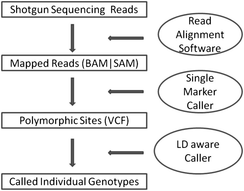
Workflow of SNP discovery and genotype calling. This figure outlines key elements in a typical variant calling pipeline in next-generation sequencing studies. The method described here focuses on the last step for refining genotypes and estimating haplotypes.

Describing chromosomes as imperfect mosaics

HMM can be used to describe the haplotypes of each individual as imperfect mosaics of other haplotypes in the sample (Li and Stephens 2003). The approach is commonly used for genotype imputation and haplotype reconstruction (Scheet and Stephens 2006; Marchini et al. 2007; Li et al. 2010) and can be extended to the analysis of short read sequence data (Li et al. 2011). In this section, we briefly review how these models can be used to model sequence data in unrelated individuals. First, haplotypes for each individual are initialized randomly—sampling an allele consistent with observed read data at each position. Then, the haplotypes of each individual are updated (in turn) using a HMM that describes the pair of haplotypes for the individual as an imperfect mosaic of other haplotypes in the sample.

To describe the model, it is sufficient to specify how haplotypes for one individual can be updated conditional on current haplotype estimates for all other individuals. For simplicity, we focus on bi-allelic markers, although our model naturally extends to markers with multiple alleles. The first step is to generate a list of candidate variant sites and to calculate P(R_i|G_i), the likelihood of observed read data R_i given an hypothetical true genotype G_i at each site i. Although we do not discuss generation of variant site lists here, we note that our method will benefit from any improvements in that stage of analysis (for example, from methods that use machine learning to discriminate likely variant sites from likely artifacts or that explicitly model transition-transversion rates and other properties of the mutation process during site discovery). Genotype likelihoods can be pre-calculated conveniently with existing tools (Li et al. 2009) and can optionally incorporate sophisticated error models, for example, to account for correlated errors (Li et al. 2008). Assuming independent errors, a simple definition for these likelihoods might be:

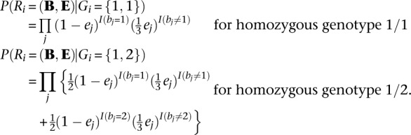Here, B and E are vectors of base calls and associated error probabilities for bases overlapping position i in the current sample (b_j and e_j are the corresponding elements) and I(expression) is an indicator function that returns 1 when expression is true and 0 otherwise.

The next step is to define P(G_i|S_i), which is the probability of an underlying true genotype G_i given mosaic state S_i. To calculate this, we use the function T(S_i), which returns the number of variant alleles in G_i or in the template haplotypes indexed by S_i. Consistent with Li et al. (2010), we define:

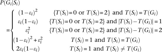Here, ɛ_i is the mosaic error rate at i^th marker, reflecting the cumulative effects of mutation and gene conversion. Together, P(R_i|G_i) and P(G_i|S_i) allow us to calculate P(R_i|S_i) as:

Finally, the last ingredient in the definition of the HMM is to define the transition probabilities P(S_{i + 1}|S_i).

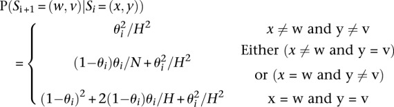Here, (x,y) and (w,v) denote indexes for the template haplotypes at position i and i + 1, θ_i denotes the mosaic transition rate between the two consecutive positions, and H denotes the number of template haplotypes under consideration.

These are all the ingredients needed to calculate P(S_i|R), the probability of a specific mosaic state at position i conditional on overlapping sequence reads R. Calculating this probability for all possible values of S_i allows us to select a pair of ordered alleles for every position (either by selecting the most likely pair or by sampling a pair according to its probability, for example). P(G_i|R), the probability of a specific genotype configuration at position i conditional on overlapping sequence reads, can be obtained by the formula

where S_i loops through all possible states. Because our model is Markovian, P(S_i|R) and P(G_i|R) can be conveniently calculated using Baum's forward-backward algorithm (Rabiner 1989), which can be implemented efficiently using recursive left and right probability functions.

Briefly, we define the left probability function L_{i + 1} as:

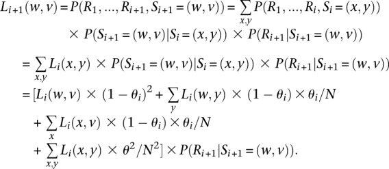At the first variant site, the function is defined as

where P(S₁ = (w,v)) is typically assumed to be a constant. Analogously, we define the right probability Q_{i+ 1}(w,v) function as:

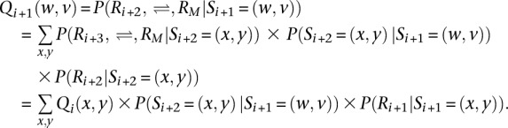At the last variant site M, the function is defined as Q_M(w,v) = 1 for convenience. Finally, we have

Joint modeling for trios

The approach described in the previous section assumes all individuals are unrelated. If related individuals are sequenced, the above model ignores important constraints on individual genotypes and haplotypes imposed by Mendel's laws. In this section, we propose a strategy for computationally efficient modeling of LD and the constraints due to Mendelian inheritance. Although this model is approximate, our simulations and empirical evaluation show that it performs well in both simulated and real data sets.

We denote R_f, R_m, and R_c as the read data, G_f , G_m, and G_c as the genotypes for the father, mother, and child in a parent-offspring trio, and the corresponding genotype likelihoods are P(R_f|G_f), P(R_m|G_m), and P(R_c|G_c). The two alleles in each genotype are ordered (Lange 2002) using the convention that the allele transmitted to the child is listed first (for parental genotypes) and that the maternal allele is listed first (for child genotypes). In principle, we could extend the previous algorithm, which is designed to sample pairs of haplotypes in unrelated individuals, to sample four haplotypes at a time in trio parents. The main weakness of this extended model would be that it requires jointly iterating over four possible haplotypes, resulting in a substantial increase in computational burden (compute costs would be proportional to H⁴ instead of H², where H is the number of haplotypes used as templates for each update). Instead, we use an approximate but computationally more tractable solution. First, we sample an ordered pair of template haplotypes and thus an ordered genotype for one of the trio parents conditional on the observed read data for the entire trio. Next, we sample an ordered pair of template haplotypes and an ordered genotype for the second parent conditional on observed read data for the trio and the sampled haplotypes for the first parent. For each iteration, the order in which the two parents are updated is selected at random.

Let 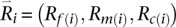denote available read information for the father, mother, and child at position i. Suppose for the current iteration we have decided to first update paternal haplotypes by sampling a mosaic state S_f(i) for the father. To do this, we replace Equation 1 with:

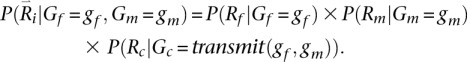
Key in evaluating this quantity is calculating the probability of the reads overlapping a particular position i conditional on a specific genotype for the father G_f = g. We define this quantity as:

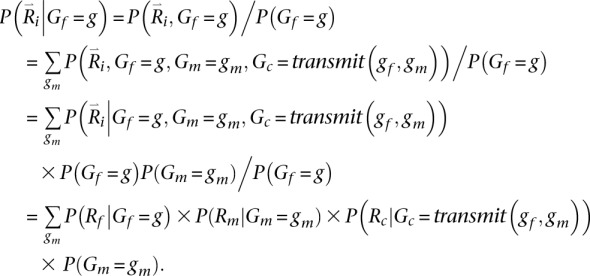Here, the transmit(G_f,G_m) function returns the genotype for the trio child conditional on ordered parental genotypes G_f and G_m. For simplicity and without loss of generality (because we iterate over all ordered parental genotypes), we specify that the first allele in the ordered genotype for each parent is transmitted to the child. While the calculation above is exact when considering a single site or when all sites are in linkage equilibrium, using it to sample haplotypes for markers in LD results in an approximate solution because, when summing over possible genotypes for the second parent, the calculation of P(G_m = g_m) does not account for dependence between genotypes at different loci.

Updates for the second parent, conditional on the sampled genotype for the first parent, also rely on a replacement for Equation 1. This time, we consider not only observed reads for the family, but also the sampled genotype for the first parent. Thus:

This expression can be evaluated using:

Summary

When dealing with samples that include trios, our algorithm thus proceeds as follows: (a) Find an initial set of haplotypes that is consistent with available read data (see Appendix A). (b) Sample a new pair of template haplotypes and corresponding genotypes for each unrelated individual. (c) For each parent-offspring pair, randomly pick one parent and sample a new pair of haplotypes for that parent. Then, sample a new pair of haplotypes for the other parent conditioning on both observed read data and haplotypes sampled for the first parent. (d) Record sampled haplotypes for every individual. (e) Optionally update estimated recombination and error rates (Li et al. 2010). (f) Repeat steps b through e.

Generating consensus haplotypes

Each round of updates generates a new pair of haplotypes for each sequenced individual. After a predefined number of rounds, a pair of consensus haplotypes for each unrelated individual is generated by finding the haplotype pair that minimizes switch error in relation to sampled haplotypes (Li et al. 2010; 2011). For parent-offspring trios, where sampled haplotypes are ordered, we generate the consensus by assigning the most frequently sampled allele at each position to the consensus haplotype.

Data sets

Simulated data

To evaluate the performance of our method, we start with simulated data sets. Simulated data allow us to assess a wide range of possibilities, varying sequencing depth, number of individuals to be sequenced, and error rates. Simulations also allow us to compare our results to a truth set. To be realistic, we simulated 10,000 haplotypes for each of one hundred 1 Mb regions using a coalescent model mimicking the LD patterns, population demographic history, and local recombination rates of European ancestry samples (Schaffner et al. 2005). Next, we randomly selected haplotypes for founders and generated haplotypes of offspring by simulating Mendelian transmission. Finally, we simulated short sequence reads assuming that depth at each site follows a Poisson distribution and defined per-base sequencing error rate. Genotype likelihoods P(R|G_i) were then calculated based on the simulated reads R.

We first simulated samples including 30 parent-offspring trios (which corresponds to 90 sequenced individuals and 60 unrelated individuals), 60 unrelated individuals, or 90 unrelated individuals. Each sample was sequenced at depth 1×, 2×, 4×, or 8× and assuming per-base error rates of 0.01 (corresponding to an average Phred scaled base quality of Q20) or 0.001 (corresponding to base quality of Q30). We also considered a second set of simulations where sample size was doubled to 60 trios, 120 or 180 unrelated individuals, and a third more limited set of simulations where the amount of sequence data to be generated was kept constant. We repeated each simulation 100 times.

Real data

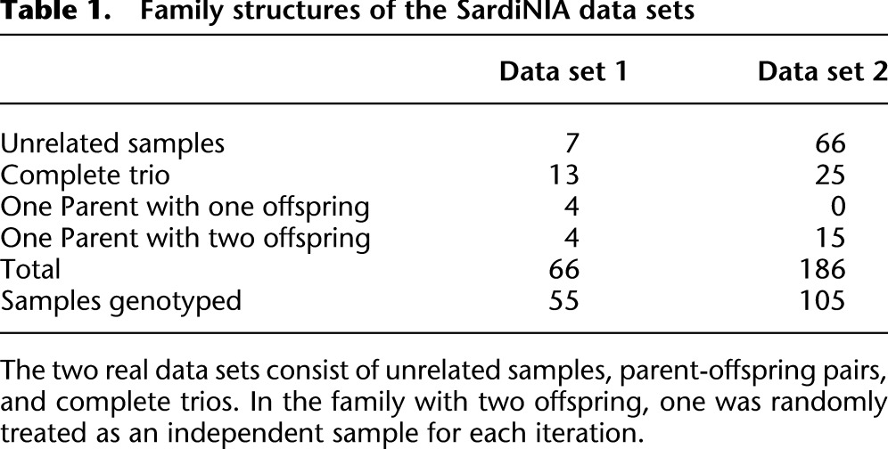
We applied this method to data from the SardiNIA Medical Sequencing Project (see http://www.ncbi.nlm.nih.gov/projects/gap/cgi-bin/study.cgi?study_id=phs000313.v1.p1). The project is a collaborative effort between the University of Cagliari, the CNR Research Institute in Pula, the University of Michigan, and the National Institute on Aging and aims to sequence 2000 Sardinian individuals at an average depth of ∼4×. Early sequencing efforts included sequencing of parent-offspring trios, parent-offspring pairs, and unrelated samples (Table 1), and our initial evaluation focused on the first 186 samples sequenced by the project at an average depth of 3.7 (which include 25 complete trios, 15 parent-offspring pairs, and 66 unrelated individuals; see Table 1) using paired end Illumina reads. To evaluate genotype accuracy, we compared genotypes derived from short read sequence data with genotypes derived using the Illumina Metabochip (Sanna et al. 2011; Voight et al. 2012), which includes many rare and common SNPs. In addition to evaluating our method, we also considered analyses using Thunder, an LD-based genotyper similar to the one described here but that ignores family structure (Li et al. 2011), and also analyses using a trio-aware single marker caller (Li et al. 2012) that ignores LD. Finally, we applied our method to the most recently finished 508 sequenced samples and evaluate the genotyping accuracy. To conserve compute resources, this larger set of 508 individuals was not analyzed with alternative genotype calling methods.

Table 1.

Family structures of the SardiNIA data sets

Performance metrics

To evaluate the performance of genotype calling, we evaluated the genotype mismatch rate between genotypes estimated using our method and gold standard genotypes, the mismatch rate at heterozygous sites, which is a more sensitive measure of accuracy for rare variants, and the squared correlation r² between estimated genotypes and gold standard genotypes. Gold standard genotypes were either the underlying simulated genotypes (for simulated data sets) or the Metabochip array genotypes (for the SardiNIA data). Since allele frequencies affect genotype call accuracy substantially, we examined the results stratified according to population frequency.

To evaluate haplotyping accuracy, we considered the number of mismatched alleles when comparing haplotypes estimated using short sequence reads and the underlying simulated haplotypes, the switch errors required to convert the estimated haplotypes into the underlying simulated haplotypes (Marchini et al. 2006), and the number of perfectly predicted haplotypes. When evaluating switch errors and perfectly predicted haplotypes, we first excluded any mismatching alleles.

Results

Overall performance

We evaluated the performance of our method in simulated and real sequencing data sets. In our view, the key insights from these comparisons arise from examining the relative performance of different analytical strategies and study designs. The absolute performance metrics will depend not only on analysis strategy but also on the population being studied, sample size, local extent of linkage disequilibrium (LD), and accuracy of read mapping.

We first evaluated the number of detected variants when different strategies were applied to simulated sequence data. As shown in Table 2 (columns 1–4), when comparing analyses of 30 trios (60 unrelated individuals, plus one offspring for each pair of individuals) with analyses that included only 60 unrelated individuals (corresponding, for example, to sequencing only the trio parents), it is clear that sequencing an additional individual per family increases the number of discovered variants at all sequencing depths examined (although the relative advantage is greater at lower depths). When we compared sequencing of 30 trios with that of 90 unrelated individuals, we observed greater numbers of detected variants in trios when depth was low (1–2×), and greater numbers of detected variants in unrelated individuals when depth was high (8×). The pattern makes intuitive sense—at higher depths, nearly all variants segregating in each family can be identified by sequencing the parents, and opportunities for detecting additional variants are maximized by sequencing additional unrelated individuals; at lower depths, some of the variants segregating in each family are missed when only parents are sequenced, and including offspring in the analysis improves power. We observed similar patterns when sample sizes were doubled to 60 trios, 120 unrelated individuals, and 180 unrelated individuals. When changing per base sequencing error rates, we observed that improving per-base error rates from 0.01 (Q20) to 0.001 (Q30) allowed us to call up to ∼10% more SNPs at the lowest depths.

Table 2.

Error rates for genotype calling in samples of parent-offspring trios or unrelated individuals, as function of sequencing depth (1×, 2×, 4×, or 8×) and per-base error rate of the original sequence traces (0.01 or 0.001)

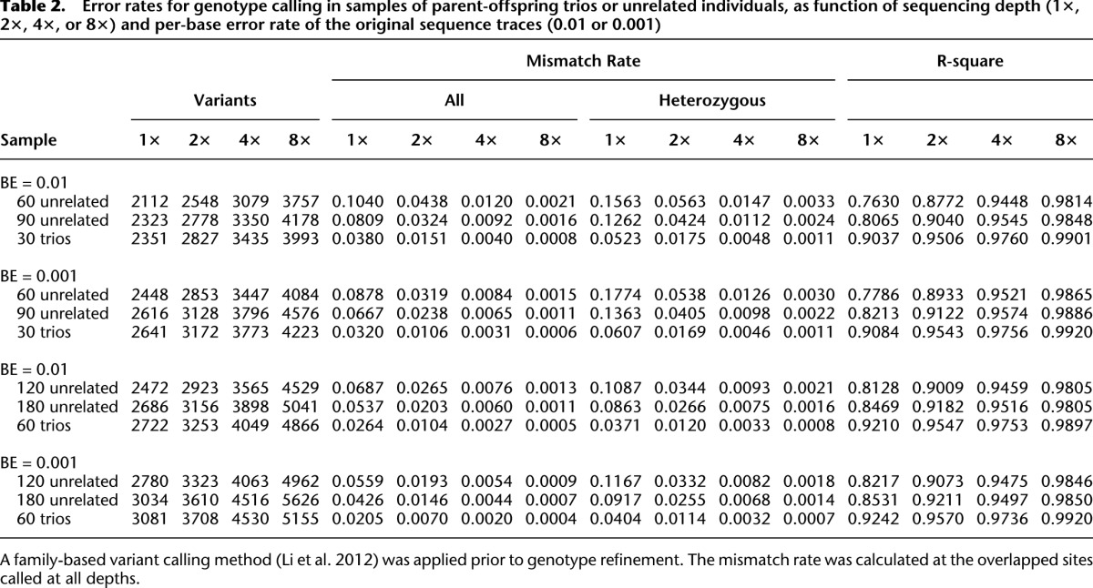
Next, we proceeded to evaluate genotype mismatch rates (Table 2, columns 5–12) and the squared correlation between simulated and estimated genotypes (Table 2, columns 13–16). Several patterns emerge: First, the advantages of sequencing trios and using our analysis method are now very clear—for any given number of sequenced individuals and depth, trios always provided the most accurate genotypes; second, genotype error rates are typically much higher at heterozygous sites—regardless of the sequencing strategy; third, increasing sample size provides substantial benefits in terms of genotype accuracy. For example, when the number of unrelated individuals increased from 60 to 120 to 180, genotype mismatch rates dropped from 4.4% to 2.7% to 2.0% at 2× coverage (and per-base error rate 0.01). Sequencing depth was also a major contributor to genotype accuracy: When 60 unrelated individuals were sequenced, error rates decreased from 10.4% to 4.4% to 1.2% and, ultimately, 0.2% as depth increased from 1× to 2× to 4× and, ultimately, 8×. Compared with the large impact of sample size and sequencing depth, increased sequencing accuracy (per-base error rate of 0.001), only, had a more modest impact on accuracy, reducing error rates by ∼20%–30%. Table 2 also exposes a counter-intuitive pattern: At very low depth (1×), decreases in per-base sequencing error rates (from 0.01 to 0.001) can increase the error rate for heterozygous genotypes. This occurs because, with more accurate data, it is possible to more aggressively call additional variant sites, although some of these newly called sites are very hard to genotype.

When comparing sequencing efforts focused on trios and on unrelated individuals, we considered two options. In one option, only the parents of trios would be sequenced (30 trios would be replaced with 60 unrelated individuals). In the second option, sequencing efforts might be kept constant (30 trios would be replaced with 90 unrelated individuals). In both cases, sequencing trios resulted in markedly lower genotype mismatch rates. For instance, the mismatch rate when 30 trios are sequenced at depth 2× (with per-base error rate of 0.001) was 1.1% compared with 2.4% and 3.2% for 90 and 60 unrelated samples, respectively. The gains in genotype accuracy provided by trios remain clear across different per base error rates, sequencing depths, and numbers of individuals sequenced. Interestingly, we note that genotype accuracy was typically slightly higher for trio offspring than for parents (Supplemental Table 2), likely because Mendelian inheritance rules place stronger constraints on offspring genotypes and because each offspring chromosome is also sequenced in the parents. For example, the mismatch rate was 0.30% for offspring and 0.45% for parents when 30 trios were sequenced at depth 4× and the simulated per-base error rate was 0.01.

The advantages of using family trios, particularly at low sequencing depths, are especially clear using the r² accuracy metric—which examines the correlation between true and estimated genotypes (and places special emphasis on rare genotypes that are hard to call). For example, with a per-base sequencing error rate of 1% and sequencing depth 1×, the r² correlation was 0.76 when 60 unrelated individuals were sequenced, 0.81 when 90 unrelated individuals were sequenced, and 0.90 when 30 trios were sequenced (corresponding to 90 total sequenced individuals, of whom 60 are unrelated). By this metric, the accuracy of sequencing 60 trios at 1× depth exceeded the accuracy of sequencing the same number of unrelated individuals at 2×, and sequencing trios at 2× outperformed sequencing of unrelated individuals at 4×. The advantages of trios are even clearer for haplotyping, discussed below.

Performance stratified by frequency

The summaries presented so far, which focus on overall summaries of genotype accuracy, mask substantial variation in genotype accuracy for different allele frequencies. The issue is illustrated in Figure 2, which summarizes genotype accuracy at heterozygous sites when 30 trios, 60 unrelated individuals, or 90 unrelated individuals are sequenced (figures for other scenarios present similar patterns and Supplemental Table 1 provides additional details). The figure makes clear that rare heterozygous sites are especially hard to call, whatever the sequencing depth; and that the relative advantages of sequencing trios are greatest for calling the rarest of these sites.

Figure 2.

Frequency stratified mismatch rate at all sites and heterozygote sites at different depths for 30 trios, 60 unrelated, and 90 unrelated samples at a base error rate of 0.01. We divided markers into allele frequency rate deciles and estimated the average mismatch rate within each bin.

Accuracy of haplotype inference

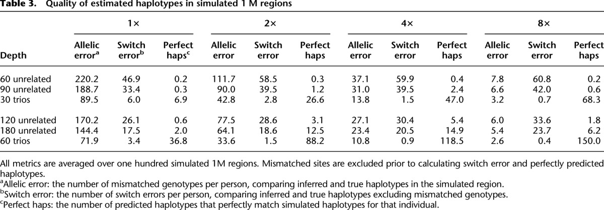
Another important advantage of our analysis methods for trio sequence data is in haplotype reconstruction, which is essential for follow-up imputation analyses and can inform inferences about population history. We evaluate the accuracy of our method by using three measures of haplotype accuracy: allelic error, switch error, and perfectly predicted haplotypes. Simulation results for one hundred 1 Mb regions are summarized in Table 3. Analogous to analyses of genotype data (Li et al. 2010), larger sample sizes increase the accuracy of estimated haplotypes. For instance, at 4× depth, analyses of 90 unrelated individuals yield 40 switch errors per simulated sample (∼1 per 25 kb), while analyses of 60 unrelated samples yield 60 switch errors per simulated sample (∼1 per 17 kb). Trios perform much better in this setting—and at 4× depth we expect <2 switch errors per simulated individual when trios are sequenced (∼1 per 600 kb). Note that, because sites with mismatching alleles are excluded from the switch error calculation, our comparison actually underestimates the relative advantages of trio sequencing. Interestingly, haplotype switch error rates sometimes increase with sequencing depth because at higher depth more rare sites, which are hardest to phase and genotype, are discovered.

Table 3.

Quality of estimated haplotypes in simulated 1 M regions

Constant sequencing effort

Supplemental Table 3 illustrates results for a design where, as an alternative to sequencing trio offspring, parents are sequenced at higher depth. In this design, the amount of sequence data to be generated is constant. Results show that increased depth provides clear benefits in terms of genotyping accuracy, so that genotyping trio parents at greater depth provides genotypes that are slightly more accurate than when sequencing effort is distributed across the family (typically, reducing genotyping error by 0%–10%). However, it is also clear that haplotyping accuracy remains much greater when trios are sequenced (eliminating 75%–98% of phasing errors).

Evaluation using SardiNIA sequencing data

The performance of our method in simulation data encouraged us to extend our evaluation to more challenging real data sets. We first analyzed the two initial sets of individuals sequenced by the Sardinia project (the first 66 sequenced individuals and the first 186 sequenced individuals, Table 1). These samples were sequenced using paired end Illumina reads to an average depth of 3.7 per sample (read lengths varied from ∼100 to ∼120 bp). Each data set was analyzed using the methods described here, and also using previously described methods that consider family structure but ignore LD (Li et al. 2012) or that model LD but ignore family structure (Li et al. 2011). Table 4 presents comparisons of genotypes derived from sequence data with those generated using Illumina Metabochip arrays (Voight et al. 2012) segregated according to Metabochip genotype; as before, we will focus our discussion on mismatch rates at hard-to-call heterozygous sites. For LD-based algorithms (whether or not family structure is modeled), larger sample sizes yield better genotype calling accuracy; in addition, the two callers that model LD seem to greatly outperform the caller that only uses population allele frequencies and family structure. For instance, in the set of 186 individuals, the single marker caller produces an error rate of ∼28.7% at heterozygous sites, compared with 5.5% for an LD-based approach ignoring relatedness and 3.7% to our approach that models both LD and allelic transmission within trios. As can be seen from the large decreases in error rate when the sample size increased from 66 individuals to 186 individuals, and consistent with other analyses (Li et al. 2011), we expect accuracy to increase further as more individuals are sequenced.

Table 4.

 Overall genotype discordance between Metabochip and low-pass sequence data from SardiNIA project

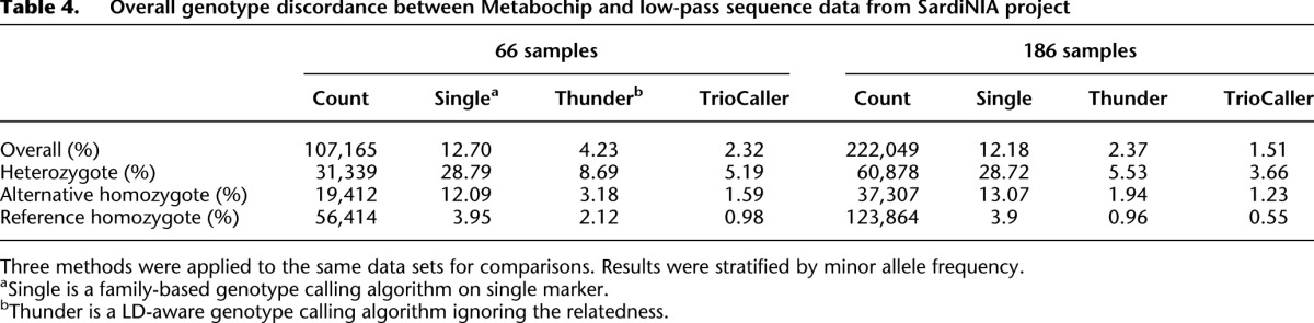
Table 5 and Figure 3 present results of the same comparisons, stratified by allele frequency and alternative allele counts. It is clear that the benefits of the LD-aware genotyping methods, which combine information across individuals sharing similar haplotypes, are greatest for common sites—where we expect many carriers of the relevant haplotypes to be present in the sample. As sample size increases, we expect these benefits to extend to rarer sites.

Table 5.

Stratified genotype discordance between Metabochip and low-pass sequence data from Sardinia project

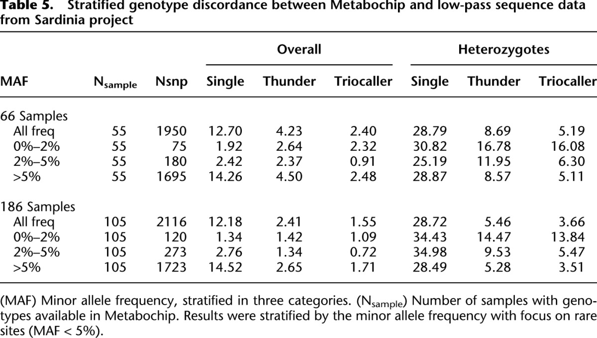
Figure 3.

Genotype distributions and discordance for heterozygotes, reference homozygotes, and alternative homozygotes. (Left) Genotype discordance between the MetaboChip and low-pass sequence data stratified by the alternative allele count. The overall concordance rate is also shown at the top. (Right) Genotype counts.

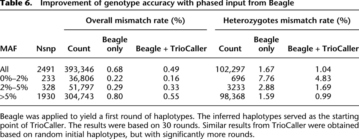
Table 6 presents updated results based on 508 recently sequenced samples. Compared with 186 samples (Table 5), the genotyping accuracy is greatly improved, especially at rarer sites. For instance, the mismatch rate for allele frequency <2% drops from 1.09% to 0.16% overall and from 13.84% to 4.83% at heterozygous sites.

Table 6.

Improvement of genotype accuracy with phased input from Beagle

Summary

Our simulations show that sequencing parent-offspring trios can greatly increase the accuracy of genotypes and haplotypes derived from next-generation sequence data, with little adverse effect on the total number of discovered variants. In addition, we show that increases in genotyping accuracy are most substantial for the rarest sites. Our results are supported not only by simulations but also by analyses of data generated by the SardiNIA sequencing study. In samples that include both trios and unrelated individuals, sequencing and appropriately analyzing some trio families also improves the accuracy of estimated genotypes for unrelated individuals in the sample (data not shown), likely because analysis of each sequenced sample is informed by preliminary haplotype estimates for the other sequenced samples.

Computational complexity

Given N sequenced, unrelated individuals, the complexity of a naïve implementation of our algorithm is O(N³), because each iteration requires that N updates and N² haplotype pairs be considered for each update. As N increases, this naïve implementation becomes extremely challenging. Thus, we also allow for the possibility that each update considers only a subset of the available haplotypes. If H haplotypes are considered (and H << N), the cost of computational cost of the algorithm is O(NH²), increasing linearly with the number of sequenced individuals N. In principle, careful attention to the choice of haplotypes included in each update should increase the accuracy of this computationally efficient implementation.

Discussion

The method presented here can accurately call genotypes and infer haplotypes for whole genome shotgun sequencing data collected in trios, unrelated individuals, or parent-offspring pairs. In addition to modeling simple family structures, our model considers haplotype stretches shared across families. In both simulated and real data, our method clearly outperforms methods that ignore LD patterns or family structure. Our method improves genotyping accuracy across the entire frequency spectrum, including both common and hard-to-call rare variants. The joint model can greatly reduce the Mendelian errors, which is crucial to the family-based association analysis.

Our method updates each parent alternatively and makes the computation feasible. Direct joint modeling of the four parental haplotypes would increase computational costs substantially, but could allow for more accurate solutions. To ascertain how much accuracy our approximation sacrifices, we also implemented this more demanding model and compared the results with our method in a small-scale simulation focused on four to eight simulated trios. In this small example, Supplemental Table 4 shows that our method results in a 5%–10% loss in accuracy while reducing computational cost by orders of magnitude (typically a factor of ∼100 running time and ∼1000 for memory use). The largest losses in accuracy from our approximation were observed at the lowest depths.

Our method includes a stochastic component, and convergence can be relatively slow. Rather than phasing every site completely at random (for an initial guess), we have found it useful to generate initial haplotypes using a computationally inexpensive method and then refine those rough haplotype estimates using our trio aware caller. This possibility is illustrated in Table 6, where we show that the hybrid approach increases the genotype accuracy, especially at the hard-to-call heterozygote sites. For instance, the mismatch rate is reduced from 1.67% to 1.04% across all sites for the same number of iterations. Using random initial haplotypes (as described in the methods section), our method would require many more iterations and computing time to achieve similar accuracy.

Our approach can be extended from trios to nuclear families with more than one offspring and, perhaps, larger pedigrees. A simple starting point might be to “split” a nuclear family into multiple trios with duplicated parents. Parents could then be updated once (according to our current scheme; conditional on a randomly selected child; or perhaps conditional on all the children) and each child could then be updated in turn conditional on the selected parental haplotypes. A key in extending our approach to larger pedigrees is to ensure that joint modeling of LD and family structure does not render any proposed approach computationally unfeasible. These investigations are beyond the scope of this paper and left for future research and experimentation.

One big advantage of our trio-aware caller is in haplotype estimation—haplotype switch error rates are reduced by >95% compared with analysis of unrelated individuals. Haplotype information can inform many genetic analyses, including LD mapping of disease genes, studies of imprinting effects and gene expression regulation, and inference about evolutionary processes such as selection and recombination. In LD mapping of disease genes, genotype imputation is often used to allow variants discovered by sequencing to be studied in additional individuals, increasing power. Since reference haplotypes are a key substrate for genotype imputation, improved haplotyping accuracy should facilitate these downstream analyses. In studies of imprinting effects and gene expression regulation, it is often important to decide whether two polymorphisms map in cis (so that their impact on the expression of nearby variants, for example, can be appropriately modeled).

The analysis presented here all focus on SNPs, but our method naturally extends to indels and other types of variants. Although a simple error model was described for the illustration purpose, more advanced models (Li et al. 2008) have potentials to improve the genotype calling. Modern tools used for site discovery (such as GATK, the Genome Analysis Toolkit [McKenna et al. 2010], and samtools [Li et al. 2009]) all have the ability to report genotype likelihoods for each sample (the probability of observed reads given an hypothetical true genotype) and store these in VCF format (Danecek et al. 2011). The resulting files can serve directly as input for our implementation of the methods described here.

Here, we have focused on genotyping and haplotyping accuracy. In addition to these, analysis of trios and other small families might provide additional advantages for design of sequencing studies (such as the ability to increase genetic load by focusing on related individuals who share a phenotype of interest or the ability to observe multiple copies of variants that are very rare in the population). The optimal mix of unrelated, trios, and other small families for human disease studies remains a fertile research area. It will also be interesting to investigate the optimal allocation of sequencing reads across a family (allowing the possibility that it may be worthwhile to sequence different family members at different depths).

The methods described here are implemented in freely available C++ code that works with standard formats (e.g., Li et al. 2009; www.1000genomes.org) and is compatible with our Michigan variant calling pipeline (a short walk-through is available online, http://genome.sph.umich.edu/wiki/TrioCaller).

Data access

The URLs for the software implementing this method presented herein are as follows: Triocaller: The C++ program based on the method described in this paper, http://genome.sph.umich.edu/wiki/TrioCaller.

Appendix

Sampling an initial haplotype set

To start our iterative haplotype estimation process, an initial guess of individual genotypes and haplotypes is needed. There are several ways to obtain the initial genotypes. We proposed two as follows.

Single site genotype calling and phasing

For each unrelated sample, individual genotypes can be sampled by calculating the posterior probabilities P(G|R) = P(R|G) × P(G)/P(R) based on the estimated population frequency P(G) and the probability of observed sequence data P(R|G). The genotype is unordered and no phase information is available from this initial guess. Therefore, when a heterozygote genotype is sampled, we order the two alleles randomly.

For parent-offspring trios, the accuracy of the initial guess can be improved by calculating posterior probabilities conditional on the whole trio. For example,

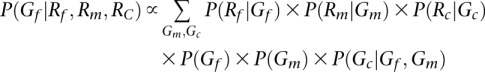Here, ordered genotypes can be sampled and initial haplotype estimates at deeply covered sites are relatively accurate, improving the convergence of the algorithm. This benefit becomes larger as sequencing depth of coverage increases.

External genotypes and haplotypes from other software

The alternative way to have an initial haplotype configuration is to run an initial analysis of data using an alternative haplotype based caller, as illustrated in the discussion.

References

- The 1000 Genomes Project Consortium 2010. A map of human genome variation from population-scale sequencing. Nature 467: 1061–1073 [DOI] [PMC free article] [PubMed] [Google Scholar]
- Cirulli ET, Goldstein DB 2010. Uncovering the roles of rare variants in common disease through whole-genome sequencing. Nat Rev Genet 11: 415–425 [DOI] [PubMed] [Google Scholar]
- Danecek P, Auton A, Abecasis G, Albers CA, Banks E, DePristo MA, Handsaker RE, Lunter G, Marth GT, Sherry ST, et al. 2011. The variant call format and VCFtools. Bioinformatics 27: 2156–2158 [DOI] [PMC free article] [PubMed] [Google Scholar]
- Eichler EE, Flint J, Gibson G, Kong A, Leal SM, Moore JH, Nadeau JH 2010. Missing heritability and strategies for finding the underlying causes of complex disease. Nat Rev Genet 11: 446–450 [DOI] [PMC free article] [PubMed] [Google Scholar]
- Hindorff LA, Sethupathy P, Junkins HA, Ramos EM, Mehta JP, Collins FS, Manolio TA 2009. Potential etiologic and functional implications of genome-wide association loci for human diseases and traits. Proc Natl Acad Sci 106: 9362–9367 [DOI] [PMC free article] [PubMed] [Google Scholar]
- Lange K. 2002. Mathematical and statistical methods for genetic analysis. Springer-Verlag, New York. [Google Scholar]
- Le SQ, Durbin R 2010. SNP detection and genotyping from low-coverage sequencing data on multiple diploid samples. Genome Res 21: 952–960 [DOI] [PMC free article] [PubMed] [Google Scholar]
- Li H, Durbin R 2009. Fast and accurate short read alignment with Burrows-Wheeler transform. Bioinformatics 25: 1754–1760 [DOI] [PMC free article] [PubMed] [Google Scholar]
- Li B, Leal SM 2008. Methods for detecting associations with rare variants for common diseases: Application to analysis of sequence data. Am J Hum Genet 83: 311–321 [DOI] [PMC free article] [PubMed] [Google Scholar]
- Li N, Stephens M 2003. Modelling Linkage Disequilibrium, and identifying recombination hotspots using SNP data. Genetics 165: 2213–2233 [DOI] [PMC free article] [PubMed] [Google Scholar]
- Li H, Ruan J, Durbin R 2008. Mapping short DNA sequencing reads and calling variants using mapping quality scores. Genome Res 18: 1851–1858 [DOI] [PMC free article] [PubMed] [Google Scholar]
- Li H, Handsaker B, Wysoker A, Fennell T, Ruan J, Homer N, Marth G, Abecasis G, Durbin R 2009. The Sequence Alignment/Map format and SAMtools. Bioinformatics 25: 2078–2079 [DOI] [PMC free article] [PubMed] [Google Scholar]
- Li Y, Willer CJ, Ding J, Scheet P, Abecasis GR 2010. MaCH: Using sequence and genotype data to estimate haplotypes and unobserved genotypes. Genet Epidemiol 34: 816–834 [DOI] [PMC free article] [PubMed] [Google Scholar]
- Li Y, Sidore C, Kang HM, Boehnke M, Abecasis GR 2011. Low-coverage sequencing: Implications for design of complex trait association studies. Genome Res 21: 940–951 [DOI] [PMC free article] [PubMed] [Google Scholar]
- Li B, Chen W, Zhan X, Busonero F, Sanna S, Sidore C, Cucca F, Kang HM, Abecasis GR 2012. A likelihood based framework for variant calling and de novo mutation detection in families for sequencing data. PLoS Genet 8: e1002944 doi: 10.1371/journal.pgen.1002944 [DOI] [PMC free article] [PubMed] [Google Scholar]
- Manolio TA, Collins FS, Cox NJ, Goldstein DB, Hindorff LA, Hunter DJ, McCarthy MI, Ramos EM, Cardon LR, Chakravarti A, et al. 2009. Finding the missing heritability of complex diseases. Nature 461: 747–753 [DOI] [PMC free article] [PubMed] [Google Scholar]
- Marchini J, Cutler D, Patterson N, Stephens M, Eskin E, Halperin E, Lin S, Qin ZS, Munro HM, Abecasis GR, et al. 2006. A comparison of phasing algorithms for trios and unrelated individuals. Am J Hum Genet 78: 437–450 [DOI] [PMC free article] [PubMed] [Google Scholar]
- Marchini J, Howie B, Myers S, McVean G, Donnelly P 2007. A new multipoint method for genome-wide association studies by imputation of genotypes. Nat Genet 39: 906–913 [DOI] [PubMed] [Google Scholar]
- McCarthy MI, Abecasis GR, Cardon LR, Goldstein DB, Little J, Ioannidis JP, Hirschhorn JN 2008. Genome-wide association studies for complex traits: Consensus, uncertainty and challenges. Nat Rev Genet 9: 356–369 [DOI] [PubMed] [Google Scholar]
- McKenna A, Hanna M, Banks E, Sivachenko A, Cibulskis K, Kernytsky A, Garimella K, Altshuler D, Gabriel S, Daly M, et al. 2010. The Genome Analysis Toolkit: A MapReduce framework for analyzing next-generation DNA sequencing data. Genome Res 20: 1297–1303 [DOI] [PMC free article] [PubMed] [Google Scholar]
- Rabiner LR 1989. A tutorial on hidden Markov-models and selected applications in speech recognition. Proc IEEE 77: 257–286 [Google Scholar]
- Roach JC, Glusman G, Smit AF, Huff CD, Hubley R, Shannon PT, Rowen L, Pant KP, Goodman N, Bamshad M, et al. 2010. Analysis of genetic inheritance in a family quartet by whole-genome sequencing. Science 328: 636–639 [DOI] [PMC free article] [PubMed] [Google Scholar]
- Sanna S, Li B, Mulas A, Sidore C, Kang HM, Jackson AU, Piras MG, Usala G, Maninchedda G, Sassu A, et al. 2011. Fine mapping of five loci associated with low-density lipoprotein cholesterol detects variants that double the explained heritability. PLoS Genet 7: e1002198 doi: 10.1371/journal.pgen.1002198 [DOI] [PMC free article] [PubMed] [Google Scholar]
- Schaffner SF, Foo C, Gabriel S, Reich D, Daly MJ, Altshuler D 2005. Calibrating a coalescent simulation of human genome sequence variation. Genome Res 15: 1576–1583 [DOI] [PMC free article] [PubMed] [Google Scholar]
- Scheet P, Stephens M 2006. A fast and flexible statistical model for large-scale population genotype data: Applications to inferring missing genotypes and haplotypic phase. Am J Hum Genet 78: 629–644 [DOI] [PMC free article] [PubMed] [Google Scholar]
- Voight BF, Kang HM, Ding J, Palmer CD, Sidore C, Chines PS, Burtt NP, Fuchsberger C, Li Y, Erdmann J, et al. 2012. The metabochip, a custom genotyping array for genetic studies of metabolic, cardiovascular, and anthropometric traits. PLoS Genet 8: e1002793 doi: 10.1371/journal.pgen.1002793 [DOI] [PMC free article] [PubMed] [Google Scholar]