Natural and Orthogonal Interaction framework for modeling gene-environment interactions with application to lung cancer

Abstract

Objectives

We aimed at extending the natural and orthogonal interaction (NOIA) framework, developed for modeling gene-gene interactions in the analysis of quantitative traits, to allow for reduced genetic models, dichotomous traits, and gene-environment interactions. We evaluate the performance of the NOIA statistical models using simulated data and lung cancer data.

Methods

The NOIA statistical models are developed for the additive, dominant, recessive genetic models, and a binary environmental exposure. Using the Kronecker product rule, a NOIA statistical model is built to model gene-environment interactions. By treating the genotypic values as the logarithm of odds, the NOIA statistical models are extended to the analysis of case-control data.

Results

Our simulations showed that power for testing associations while allowing for interaction using the statistical model is much higher than using functional models for most of the scenarios we simulated. When applied to the lung cancer data, much smaller P-values were obtained using the NOIA statistical model for either the main effects or the SNP-smoking interactions for some of the SNPs tested.

Conclusion

The NOIA statistical models are usually more powerful than the functional models in detecting main effects and interaction effects for both quantitative traits and binary traits.

Introduction

Although genome-wide association studies (GWAS) have been successful in identifying disease susceptibility loci, it remains a challenging goal for statistical geneticists to identify and characterize effects of genetic and environmental factors that influence common complex traits [1, 2]. The significant SNP associations identified by GWAS are estimated to account for only a few percent of the genetic variance [3, 4]. Since most of these studies have used a single-locus analysis strategy, there is increasing interest in genome-wide interaction analysis in the efforts of finding the missing heritability. An important issue is how one can properly quantify the genetic and environmental effects in a unified manner such that correct estimation can be achieved for the relative contributions of different factors. This is the case especially when there exist gene-gene or gene-environment interactions.

The term GxE interaction has various different meanings. The nature of an interaction may be biological or merely statistical. A statistical interaction may be defined as departure from an additive model on some scale. For a quantitative trait, if the contributions of a genetic locus and an environment factor are additive on the scale of this trait, we say that there is no interaction between the locus and the environment factor. Any deviation from this additivity will be referred to as a GxE interaction. For a binary trait (such as a disease), we define the GxE interaction as deviation from additivity of a genetic effect and an environment effect on the log-odds scale.

The statistical formulation of the natural and orthogonal interaction (NOIA) model of genetic effects, were recently developed [5] and provides a framework in which estimates of genetic effects for a quantitative trait remain orthogonal even under the departure from Hardy-Weinberg proportions (HWP) of the loci. The orthogonal estimates do not change in a reduced model and hence are very convenient for model selection for finding the genetic architecture of the traits[6]. More importantly, the NOIA framework directly leads to a proper and orthogonal decomposition of genetic variance and hence a more meaningful calculation of the heritability of the trait, while facilitating the modeling of multiple genetic factors along with their interactions.

In this paper, we evaluate the performance of the orthogonal models, compared to the usual models, in both testing for interaction between two factors and testing for association while allowing for interaction. We extend the NOIA framework in several different ways. First, we derive the NOIA formulation to all possible reduced genetic models, including the additive, dominant and recessive models. We then extend the NOIA framework to include a binary environmental exposure and its interaction with a gene with a reduced or saturated genetic model. Finally, we also explore the possibility of generalizing the orthogonal models to the analysis of binary traits, such as diseases. We found that the meaning of orthogonality is somewhat different on the log-odds scale than its original meaning for a quantitative trait: although the estimators are no longer orthogonal, the variance decomposition remains orthogonal when the log-odds are simply treated as genetic effects under the alternative hypothesis of an effect in the NOIA formulation. Our simulation results showed that for both quantitative and qualitative traits, the statistical models have higher power than the usual functional ones in most of the scenarios we have tested. We also illustrate the usage of the formulations using real data.

Methods

One-locus models: quantitative traits

If a quantitative trait is influenced by a single diallelic gene, or locus,

$$Y=G+e,$$ (1)

the genotypic value can be modeled using linear regression on the number of a reference allele, say allele 2, as follows:

$$G=\mu +(N-\overline{N})\alpha +\mathit{\epsilon \delta },$$ (2)

where G = G₁₁, G₁₂ and G₂₂ are the genotypic values when the number of reference alleles is, N = 0, 1 and 2, respectively, and

$$\epsilon =\{\begin{array}{c}-2p_{12}{p}_{22}/V\\ 4p_{11}{p}_{22}/V\\ -2p_{11}{p}_{12}/V\end{array}$$ (3)

with genotype frequencies p₁₁, p₁₂ and p₂₂, respectively. Here N̄ and V denote the mean and variance of N

$$\begin{array}{lll}\overline{N}& =& p_{12}+2p_{22}\\ V& =& p_{12}+2^2{p}_{22}-{(p_{12}+2p_{22})}^2=p_{11}+p_{22}-{(p_{11}-p_{22})}^2,\end{array}$$

respectively. The genetic effect vector, ${\overrightarrow{E}}_s$, consists of the three regression parameters, μ = Ḡ, α = COV(N, G)/V and δ = G₁₂ − (G₁₁ + G₂₂)/2, and can be expressed as

$${\overrightarrow{E}}_s\equiv \left(\begin{array}{c}\mu \\ \alpha \\ \delta \end{array}\right)=\left(\begin{array}{ccc}{p}_{11}& p_{12}& p_{22}\\ p_{11}^{\prime }& p_{12}^{\prime }& p_{22}^{\prime }\\ -\frac{1}{2}& 1& -\frac{1}{2}\end{array}\right)\left(\begin{array}{c}{G}_{11}\\ G_{12}\\ G_{22}\end{array}\right),$$ (4)

if we define

$$p_{\mathit{ij}}^{\prime }=p_{\mathit{ij}}\frac{N_{\mathit{ij}}-\overline{N}}{V}.$$ (5)

The vector of genotypic values, $\overrightarrow{G}$, can be expressed by

$$\left(\begin{array}{c}{G}_{11}\\ G_{12}\\ G_{22}\end{array}\right)=S_s{\overrightarrow{E}}_s=\left(\begin{array}{ccc}1& -\overline{N}& -2p_{12}{p}_{22}/V\\ 1& 1-\overline{N}& 4p_{11}{p}_{22}/V\\ 1& 2-\overline{N}& -2p_{11}{p}_{12}/V\end{array}\right)\left(\begin{array}{c}\mu \\ \alpha \\ \delta \end{array}\right).$$ (6)

Here, S_s is the design matrix. In a regression analysis, we make inference on parameters (μ, α and δ). Therefore S_s can also be referred to as coding matrix for sampled data, because each row of S_s includes the code for regression on the parameters for an individual with the corresponding genotype. For example, if an individual has genotype 12, data for this individual will be coded according to the second row of S_s as follows:

$$G=\mu +(1-\overline{N})\alpha +\frac{4p_{11}{p}_{22}}{V}\delta .$$ (7)

Unlike the genotypic values, $\overrightarrow{G}$, the genetic effects, ${\overrightarrow{E}}_s$, depend on genotype frequencies and the model based on these parameters are referred to as statistical model [5]. As shown in [5], this statistical model is orthogonal, meaning that estimates of these parameters are uncorrelated. The orthogonality of the statistical model is also reflected by the fact that the variance of G can be decomposed into those of the additive and dominant components

$$V_G=\mathrm{Var}[(N-\overline{N})\alpha ]+\mathrm{Var}[\mathit{\epsilon \delta }]$$ (8)

because COV[(N − N̄)α, εδ] = 0. The additive and dominant variances can be expressed as

$$V_{\alpha }={\alpha }^{2}V$$ (9)

$$V_{\delta }=4p_{11}{p}_{12}{p}_{22}{\delta }^2(p_{12}{p}_{22}+4p_{11}{p}_{22}+p_{11}{p}_{12})/V.$$ (10)

Traditionally, the one-locus genotypes are coded in one of the following two ways: (−1, 0, 1) and (0, 1, 2). In either case, the genetic effects do not depend on allele frequencies and are determined merely by the functionality of the locus. So, both coding methods correspond to functional models. For these two coding schemes, the genotypic values are expressed as

$$\left(\begin{array}{c}{G}_{11}\\ G_{12}\\ G_{22}\end{array}\right)=\left(\begin{array}{ccc}1& -1& 0\\ 1& 0& 1\\ 1& 1& 0\end{array}\right)\left(\begin{array}{c}R\\ a\\ d\end{array}\right)=S_1{\overrightarrow{E}}_1,$$ (11)

and

$$\left(\begin{array}{c}{G}_{11}\\ G_{12}\\ G_{22}\end{array}\right)=\left(\begin{array}{ccc}1& 0& 0\\ 1& 1& 1\\ 1& 2& 0\end{array}\right)\left(\begin{array}{c}R\\ a\\ d\end{array}\right)=S_2{\overrightarrow{E}}_2,$$ (12)

respectively. These two functional models are related to the statistical model through

$$\left(\begin{array}{c}\mu \\ \alpha \\ \delta \end{array}\right)=\left(\begin{array}{ccc}1& p_{22}-p_{11}& p_{12}\\ 0& 1& p_{12}^{\prime }\\ 0& 0& 1\end{array}\right)\left(\begin{array}{c}R\\ a\\ d\end{array}\right),$$ (13)

and

$$\left(\begin{array}{c}\mu \\ \alpha \\ \delta \end{array}\right)=\left(\begin{array}{ccc}1& \overline{N}& p_{12}\\ 0& 1& p_{12}^{\prime }\\ 0& 0& 1\end{array}\right)\left(\begin{array}{c}R\\ a\\ d\end{array}\right),$$ (14)

respectively. In contrast to the statistical model, neither of these two functional models is orthogonal.

One-locus models: qualitative traits

For the analysis of cas-control data sampled according to a qualitative trait such as disease, we can define a similar statistical model by treating the genotypic values and the genetic effects as the logit (i.e., logarithm of the odds) of the disease. However, two important features of the orthogonal models may no longer be valid here. First, the estimates of parameters using logistic regression are not uncorrelated. Recall that the variance of estimates of parameters for linear regression can be expressed as

$$\mathrm{Var}(\overrightarrow{\beta })={\sigma }^2{\left({\chi }^{\mathrm{T}}\chi \right)}^{-1},$$ (15)

where χ is the design matrix, as far as the error terms for all samples are independent and identically distributed with variance σ², which can be shown to be diagonal for the statistical model [5]. However, for logistic regression, the variance of estimates of parameters is

$$\mathrm{Var}(\overrightarrow{\beta })={\left({\chi }^{\mathrm{T}}\mathit{\nu \chi }\right)}^{-1}$$ (16)

where ν is a diagonal matrix with elements

$${\pi }_{G_i}(1-{\pi }_{G_i})$$ (17)

for the ith individual in the sample with π_Gi the probability of being affected given the values of regressor for the individual. It can be shown that

$${\chi }^{\mathrm{T}}\mathit{\nu \chi }=n{S}^{\mathrm{T}}D\prime S$$ (18)

where

$$D^{\prime }=\left(\begin{array}{ccc}{\pi }_{11}(1-{\pi }_{11})p_{11}& 0& 0\\ 0& {\pi }_{12}(1-{\pi }_{12})p_{12}& 0\\ 0& 0& {\pi }_{22}(1-{\pi }_{22})p_{22}\end{array}\right),$$ (19)

and S is a design matrix. This means that, for logistic regression, the statistical model defined in (6) has no orthogonal estimates as in the case of linear regression, unless the gene is not associated with the disease (π_G would then assume the same values for all genotypes). Second, as will be shown later, the estimates of main effects for a full interaction model is no longer the same as the corresponding effects of the reduced models, i.e., the single-locus model and the environment-only models. Nevertheless, the orthogonal decomposition of variance is still valid here on the log-odds scale. We will therefore apply this model to the analysis of case-control data. We will hereafter use a common terminology, statistical model, for both quantitative and qualitative trait, and evaluate its performance in simulation studies. We do not explicitly model the influence of the genotype frequencies on the variance of the regression parameters in logistic regression.

We extended the formulations for the statistical and functional models to the following three reduced genetic models: additive, dominant, and recessive.

Gene-environment interaction

Suppose we have a binary environmental exposure, M, with phenotypic values M₁ and M₂ for unexposed and exposed individuals, respectively. Denote the unexposed frequency by m. A functional model for this environmental exposure is

$$\overrightarrow{M}=\left(\begin{array}{c}{M}_1\\ M_2\end{array}\right)=\left(\begin{array}{cc}1& 0\\ 1& 1\end{array}\right)\left(\begin{array}{c}R\\ a_M\end{array}\right),$$ (20)

with effects defined as

$${\overrightarrow{E}}_M=\left(\begin{array}{c}R\\ a_M\end{array}\right)=\left(\begin{array}{cc}1& 0\\ -1& 1\end{array}\right)\left(\begin{array}{c}{M}_1\\ M_2\end{array}\right).$$ (21)

For a two-level factor, following [5], the criterion for orthogonality can be derived as follows. From the regression model

$$\left(\begin{array}{c}{M}_1^{\ast }\\ M_2^{\ast }\\ ⋮\hfill \\ M_n^{\ast }\end{array}\right)=\left(\begin{array}{cc}1& 0\\ 0& 1\\ ⋮& ⋮\\ 0& 1\end{array}\right)\left(\begin{array}{c}{M}_1\\ M_2\end{array}\right)=\sout{Z}S\overrightarrow{E}=\chi \overrightarrow{E}$$ (22)

orthogonality requires that

$${\chi }^{\mathrm{T}}\chi =n{S}^{\mathrm{T}}{\sout{Z}}^{\mathrm{T}}\sout{Z}S=S^{\mathrm{T}}\mathit{DS}$$ (23)

is diagonal, where

$$D=\left(\begin{array}{cc}{m}_1& 0\\ 0& m_2\end{array}\right),$$ (24)

and m₁ = m and m₂ = 1 − m are the exposure frequencies. Since

$${\chi }^{\mathrm{T}}\chi =n\left(\begin{array}{cc}{m}_1{s}_{11}^2+m_2{s}_{21}^2& m_1{s}_{11}{s}_{12}+m_2{s}_{21}{s}_{22}\\ m_1{s}_{11}{s}_{12}+m_2{s}_{21}{s}_{22}& m_1{s}_{12}^2+m_2{s}_{22}^2\end{array}\right)$$ (25)

it follows that the model, S, is orthogonal when

$$m_1{s}_{11}{s}_{12}+m_2{s}_{21}{s}_{22}=0.$$ (26)

Using this criterion, we find that the functional model given above is not orthogonal.

The orthogonal (or, statistical) model for the binary environmental factor is

$$\overrightarrow{M}=\left(\begin{array}{c}{M}_1\\ M_2\end{array}\right)=\left(\begin{array}{cc}1& m-1\\ 1& m\end{array}\right)\left(\begin{array}{l}\mu \\ {\alpha }_M\end{array}\right),$$ (27)

with effects defined as

$${\overrightarrow{E}}_M=\left(\begin{array}{l}\mu \\ {\alpha }_M\end{array}\right)=\left(\begin{array}{cc}m& 1-m\\ -1& 1\end{array}\right)\left(\begin{array}{c}{M}_1\\ M_2\end{array}\right).$$ (28)

Using the Kronecker product rule [5], we have the following non-orthogonal functional model for the gene-environment interaction

$${\overrightarrow{G}}_{\mathit{GM}}=\left(\begin{array}{c}{G}_{11M_1}\\ G_{12M_1}\\ G_{22M_1}\\ G_{11M_2}\\ G_{12M_2}\\ G_{22M_2}\end{array}\right)=\left(\begin{array}{cccccc}1& 0& 0& 0& 0& 0\\ 1& 1& 1& 0& 0& 0\\ 1& 2& 0& 0& 0& 0\\ 1& 0& 0& 1& 0& 0\\ 1& 1& 1& 1& 1& 1\\ 1& 2& 0& 1& 2& 0\end{array}\right)\left(\begin{array}{l}R\\ a_G\\ d_G\\ a_M\\ \mathit{aa}\\ \mathit{da}\end{array}\right),$$ (29)

and the statistical model

$${\overrightarrow{G}}_{\mathit{GM}}=\left(\begin{array}{cccccc}1& -\overline{N}& -2p_{12}{p}_{22}/V& m-1& -(m-1)\overline{N}& -2(m-1)p_{12}{p}_{22}/V\\ 1& 1-\overline{N}& 4p_{11}{p}_{22}/V& m-1& (m-1)(1-\overline{N})& 4(m-1)p_{11}{p}_{22}/V\\ 1& 2-\overline{N}& -2p_{11}{p}_{12}/V& m-1& (m-1)(2-\overline{N})& -2(m-1)p_{11}{p}_{12}/V\\ 1& -\overline{N}& -2p_{12}{p}_{22}/V& m& -m\overline{N}& -2m{p}_{12}{p}_{22}/V\\ 1& 1-\overline{N}& 4p_{11}{p}_{22}/V& m& m(1-\overline{N})& 4m{p}_{11}{p}_{22}/V\\ 1& 2-\overline{N}& -2p_{11}{p}_{12}/V& m& m(2-\overline{N})& -2m{p}_{11}{p}_{12}/V\end{array}\right)\left(\begin{array}{l}\mu \\ {\alpha }_G\\ {\delta }_G\\ {\alpha }_M\\ \mathit{\alpha \alpha }\\ \mathit{\delta \alpha }\end{array}\right).$$ (30)

The relation between the statistical and functional models is

$$\left(\begin{array}{l}\mu \\ {\alpha }_G\\ {\delta }_G\\ {\alpha }_M\\ \mathit{\alpha \alpha }\\ \mathit{\delta \alpha }\end{array}\right)=\left(\begin{array}{cccccc}1& \overline{N}& p_{12}& 1-m& (1-m)\overline{N}& (1-m)p_{12}\\ 0& 1& p_{12}^{\prime }& 0& 1-m& (1-m)p_{12}^{\prime }\\ 0& 0& 1& 0& 0& 1-m\\ 0& 0& 0& 1& \overline{N}& p_{12}\\ 0& 0& 0& 0& 1& p_{12}^{\prime }\\ 0& 0& 0& 0& 0& 1\end{array}\right)\left(\begin{array}{l}R\\ a_G\\ d_G\\ a_M\\ \mathit{aa}\\ \mathit{da}\end{array}\right).$$ (31)

One of the desired properties of the statistical models is that the marginal effects of the gene or the environmental exposure are the same as the corresponding main effects of the full GxE model. This is the case for the linear regression of a quantitative trait. For a quantitative trait determined by a gene and a binary exposure, from the vector of genotypic values, $\overrightarrow{G}={(G_{11M_1},G_{12M_1},G_{22M_1},G_{11M_2},G_{12M_2},G_{22M_2})}^{\mathrm{T}}$, the marginal model for the gene is

$$G_{11}^{\prime }=m{G}_{11M_1}+(1-m)G_{11M_2}$$ (32)

$$G_{12}^{\prime }=m{G}_{12M_1}+(1-m)G_{12M_2}$$ (33)

$$G_{22}^{\prime }=m{G}_{22M_1}+(1-m)G_{22M_2}.$$ (34)

It can be shown that the corresponding marginal genetic effects is

$$\left(\begin{array}{c}{\mu }^{\prime }\\ {\alpha }^{\prime }\\ {\delta }^{\prime }\end{array}\right)=\left(\begin{array}{ccc}{p}_{11}& p_{12}& p_{22}\\ p_{11}^{\prime }& p_{12}^{\prime }& p_{22}^{\prime }\\ -\frac{1}{2}& 1& -\frac{1}{2}\end{array}\right)\left(\begin{array}{c}{G}_{11}^{\prime }\\ G_{12}^{\prime }\\ G_{22}^{\prime }\end{array}\right)=\left(\begin{array}{c}{\mu }_G\\ {\alpha }_G\\ {\delta }_G\end{array}\right).$$ (35)

A similar expression can be obtained for the marginal effects of the environmental exposure. However, this may not be the case for the statistical model under the alternate model of association defined on the log-odds scale for a qualitative trait. This is because the same relation for the genotypic values, equations (32),(33), and (34), is valid on the scale of penetrance, and the penetrances are nonlinearly related to the log-odds.

For the three reduced genetic models, the formulations for statistical and functional models for GxE and their relationships are given in Supplementary Note.

Simulation methods

Simulation of data with a quantitative trait

It is straightforward to simulate data of independent individuals randomly sampled with a quantitative trait influenced by a diallelic gene and a binary exposure. For given values of the variant allele frequency, p, and the exposure prevalence, m, assuming independency between the gene and the exposure and Hardy-Weinburg proportion for the gene, an individual was assigned joint genotype 111, 121, 221, 112, 122, or 222 with probabilities, p²(1 − m), 2p(1 − p)(1 − m), (1 − p)²(1 − m), p²m, 2p(1 − p)m or (1 − p)²m, respectively. Each individual was then assigned a value of the quantitative trait according to the genotypes using the genotypic values determined from a pre-specified vector of genetic effects: ${\overrightarrow{E}}^{\mathrm{T}}=[R,a_G,d_G,a_M,\mathit{aa},\mathit{da}]$. A residual was then added to the simulated quantitative trait by generating a random number from a normal distribution with pre-specified mean (0) and variance ( ${\sigma }_e^2$). Data so simulated for 1000 individuals served as a replicate. For each genetic model, 1000 replicates were simulated.

Simulations of case-control data

We simulated case-control data with both main and interaction effects using the logistic models. If the risk of disease is determined by a diallelic gene and a binary exposure, we assume that the penetrance model is given by

$$\mathrm{Pr}(d=1\mid i)=\frac{1}{1+\exp (-G_i)},$$ (36)

where d = 1 denotes that fact that an individual is affected and G_i is the genotypic value when the joint genotype is i with i = 111, 121, 221, 112, 122, or 222. Using Bayes’ theorem, we have the distribution of the six genotypes in the cases as follows

$$\mathrm{Pr}(i\mid d=1)=\frac{P_i/[1+\exp (-G_i)]}{{\sum }_j{P}_j/[1+\exp (-G_j)]},$$ (37)

where P_i is the frequency of genotype i in the population, given by p²(1 − m), 2p(1 − p)(1 − m), (1 − p)²(1 − m), p²m, 2p(1 − p)m or (1 − p)²m, respectively, as in the simulation of a quantitative trait. Given the genotypic values and the frequencies of the joint genotypes, this expression was used for simulating joint genotypes of cases. For the simulation of controls, we have a similar expression:

$$\mathrm{Pr}(i\mid d=0)=\frac{P_i/[1+\exp (G_i)]}{{\sum }_j{P}_j/[1+\exp (G_j)]}.$$ (38)

The genotypic values were determined from pre-specified genetic effects, $\overrightarrow{E}$. It should be noted that, unlike the simulated data for a quantitative trait, not only the allele frequencies, but also the genetic effects, in the simulated case-control data are usually different from the corresponding pre-specified values (population parameters) because of ascertainment bias.

Results

Results of simulations

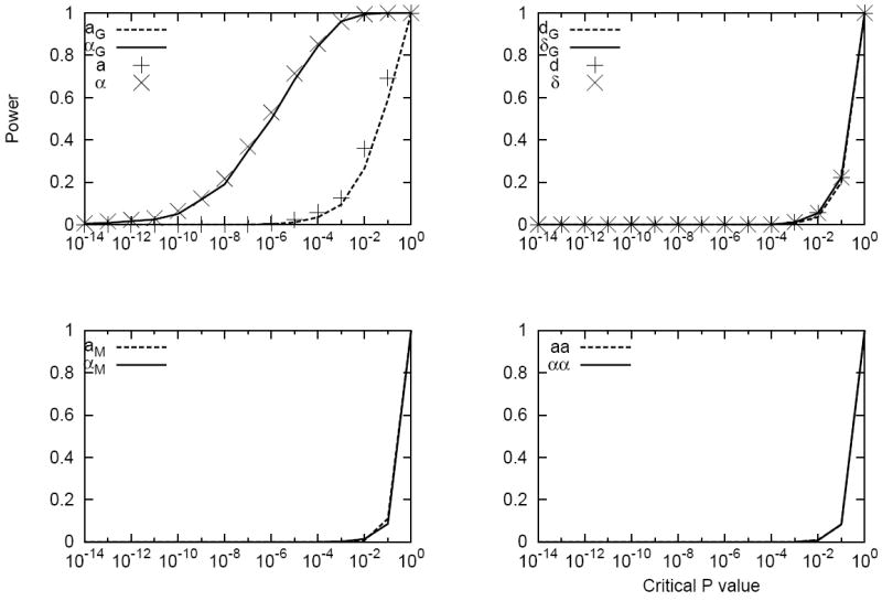
Our first simulation exhibited both main effects of a gene and a binary exposure and their interaction on a quantitative trait, representing a general scenario: ${\overrightarrow{E}}^{\mathrm{T}}=[R,a_G,d_G,a_M,\mathit{aa},\mathit{da}]=[100.0,4.0,1.0,3.0,2.0,1.5]$. The residual variance was 144.0, and the allele frequency and exposure frequency were 0.15 and 0.22 respectively. The vector of genetic effects in the statistical model was then [102.33, 5.37, 1.33, 3.98, 3.05, 1.5]. Figure S1 shows the distribution of the estimates of all six effects in all the 1000 replicates. It can be seen that for both the statistical and the functional models, the vectors of genetic effects were estimated accurately. Figure 1 shows the power as a function of critical values of the Wald test P-values for the four parameters: the additive effects of the gene, the dominant effects of the gene, the environment effect, and the interaction effect between the additive effect of the gene and the environment effect for both statistical models and functional models. For the dominant by environment interaction effects, the estimates and the test P-values were identical for the statistical and functional models. Also shown is the power for the additive and dominant effects of the gene using the gene-only statistical models. It is clear that for the additive effect of the gene, both the GxE model and the gene-only model had much higher power than the functional models. For the environment effect, the statistical model had higher power than the functional model.

Fig. 1.

Power vs. critical values of the Wald testing P-values as a test statistic for a simulated data set with a quantitative trait influenced by a gene and an environmental factor. The simulating values of the genetic effects were ${\overrightarrow{E}}^{\mathrm{T}}=[100.0,4.0,1.0,3.0,2.0,1.5]$. The corresponding statistical genetic effects were [102.33, 5.37, 1.33, 3.98, 3.05, 1.5]. The allele frequency and exposure frequency were 0.15 and 0.22, respectively. The simulating residual variance is 144.0.

Another simulation was performed for a scenario where only the gene was responsible to the trait: ${\overrightarrow{E}}^{\mathrm{T}}=[100.0,4.0,2.0,0.0,0.0,0.0]$. The residual variance was 144.0 and the allele frequency and exposure frequency were 0.15 and 0.22 respectively. The vector of genetic effects in the statistical model was then [101.71, 5.40, 2.00, 0.00, 0.00, 0.00]. Again, the estimates of parameters were accurate, as shown in Figure S2, for both the statistical and functional models. For the additive effect of the gene and the additive by environment interaction effect, the estimate of the statistical model had less variations among the replicates than that of the functional model. Power for detecting the additive effect was again much higher in the statistical model than that in the functional model (Figure 2). Power for detecting the dominant effects using both statistical and functional models were very low because of the small simulating value compared to the residual variance (2 vs. 144). For the other two parameters, for which the simulating values were zero, the false positive rates were very close to the nominal value for both statistical and functional models.

Fig. 2.

Power vs. critical values of the Wald testing P-values as a test statistic for a simulated data set with a quantitative trait influenced by a gene and an environmental factor. The simulating values of the genetic effects were ${\overrightarrow{E}}^{\mathrm{T}}=[100.0,4.0,2.0,0.0,0.0,0.0]$. The corresponding statistical genetic effects were [101.71, 5.40, 2.00, 0.00, 0.00, 0.00]. The allele frequency and exposure frequency were 0.15 and 0.22, respectively. The simulating residual variance is 144.0.

Similar scenarios were simulated for a qualitative trait. For a generic scenario, we used a vector of genetic effects given by [−2.0, 0.3, 0.1, 0.2, 0.1, 0.04]. The allele frequency and exposure frequency were set to 0.25 and 0.25, respectively. Because we simulated case-control data set, the ascertainment of equal number of cases and controls altered the proportions of being affected for different genotypes and exposure status. The resulting genetic effects, averaged over all 1000 replicates in the sample were thus estimated as [−0.26, 0.28, 0.10, 0.18, 0.27, −0.15], referred to as the actual functional effects. The statistical effects were then calculated using the actual allele frequency and exposure frequency and the actual functional effects: [0.00, 0.38, 0.06, 0.26, 0.20, −0.15]. Figure S3 shows that this actual (or, sample) statistical effects were indeed located in the corresponding center of the distribution of estimated parameters using logistic regression. Also shown in Figure S3 is that the functional model correctly estimated the actual genetic effects. Figure 3 shows that power of detecting the main additive effect of the gene was mush higher than that of the functional model. Power of detecting the exposure effect using the statistical model was also significantly higher than the functional model. For the dominant effect and the interaction effect, both models had the similarly low power.

Fig. 3.

Power vs. critical values of the Wald testing P-values as a test statistic for a simulated case-control data set with GxE interaction for all replicates. The simulating values of the genetic effects were ${\overrightarrow{E}}^{\mathrm{T}}=[-2.0,0.3,0.1,0.2,0.1,0.04]$. The actual sample values of the genetic effects were [−0.28, 0.30, 0.10, 0.20, 0.11, 0.03]. The corresponding statistical genetic effects were [−0.01, 0.38, 0.10, 0.27, 0.13, 0.03]. The allele frequency and exposure frequency were 0.25 and 0.25 respectively.

Similar to the case of quantitative trait, we also simulated case-control data a scenario where only the gene was associated to the disease with simulating values of genetic effects given by [−2.0, 0.4, 0.2, 0.0, 0.0, 0.0]. The allele frequency and exposure frequency were still set to 0.25 and 0.25, respectively. Again because of ascertainment, the sample genetic effects were actually [−0.27, 0.35, 0.23, −0.08, −0.02, 0.05] and the corresponding statistical effects where [0.00, 0.45, 0.25, −0.07, 0.00, 0.05]. Figure S4 shows the distributions of estimates of the parameters from analyses using the statistical and functional models.

In the four simulations given above, the difference of powers between the NOIA statistical models and the functional models were extremely large. For instance, in Figure 1, it can be seen that the power for testing α = 0 was about 95% and the power for testing for a = 0 was only around 30% at the 1% significance level. The power of tests depends on many factors, including allele frequencies, sample sizes, genetic effects, and significance level. We plotted power for a wide range of significance level, which allows one to compare tests of powers of tests across a broad range. We use these simulations to illustrate how the transformation from the usual functional model to the statistical model may improve power of detecting a genetic factor.

For both quantitative and qualitative traits, we also simulated the null scenario, that is, a scenario without any effects either from the gene or the environmental factor (data not shown), and found that all the false positive rates were around the nominal level.

Application to real dataset

We applied the NOIA statistical model and the usual functional model to the ILCCO (International lung cancer consortium) data [7], consisting of 17 independent case-control studies (most but not all of the original studies agreed to participate in this study). The objectives of the consortium are to share data to increase statistical power, reduce duplication of research efforts, replicate novel findings, and realize substantial cost savings. Details of the participating studies have been described previously [7]. Our goal here was to examine how genetic variants, which have been identified through GWAS, may interact with smoking in determining the risk of lung cancer by pooling the datasets. Here, we focused on six SNPs in three regions: rs2736100 and rs402710 (5p15), rs2256543 and rs4324798 (6p21), and rs16969968 and rs8034191 (15q25). Our analysis included 95468 Caucasians with 39686 cases and 55752 controls after quality control. For both NOIA statistical model and the usual functional model, logistic regression was performed with sex, age and study group as covariates.

Table 1 and Table S1 show the P-values and estimates and their 95% confidence intervals of the analysis, respectively. For the four SNPs located on 5p15 and 15q25, the NOIA statistical model detected genetic additive effects, while the functional model did not or showed larger P-values. For the additive-smoking interaction effects, the NOIA statistical model was more powerful than the functional one for the two SNPs on 15q25 and SNP rs2256543 on 6q21. For all SNPs and all models, the smoking effect was extremely significant. But, here the NOIA statistical models showed much smaller P-values than the functional models. For the covariates, sex and age, results from statistical and functional models were the same, as they were modeled in the same way. None of the SNPs had significant dominant effects, or dominant-smoking interaction, under either statistical model or functional model. It is interesting that the SNP rs2256543 on 6p21 was detected to predict lung cancer risk through an interaction with smoking, but no main effect.

Table 1.

P-values for the main effects and interactions^a

	Model	Add	Dom	SM	Add-SM	Dom-SM	Sex	Age
rs2736100	Func	0.0005	0.7	1.6e-72	0.3	0.7	9.1e-09	1.7e-16
5p15	Stat	1.9e-10	1	3.5e-267	0.3	0.7	9.1e-09	1.7e-16
rs402710	Func	0.09	1	3.2e-125	0.8	0.9	7.0e-09	3.1e-37
5p15	Stat	2.3e-08	0.8	4.4e-244	0.7	0.9	7.0e-09	3.1e-37
rs2256543	Func	0.2	0.6	1.3e-84	0.06	0.4	6.6e-09	4.9e-16
6p21	Stat	0.5	0.7	1.2e-271	0.04	0.4	6.6e-09	4.9e-16
rs4324798	Func	0.8	0.6	5.6e-227	0.8	0.8	2.9e-08	5.9e-29
6p21	Stat	0.4	0.4	2.9e-270	0.3	0.8	2.9e-08	5.9e-29
rs16969968	Func	1	0.9	6.0e-96	0.0007	0.6	4.1e-08	3.5e-28
15q25	Stat	7.4e-16	0.1	6.9e-266	9.5e-05	0.6	4.1e-08	3.5e-28
rs8034191	Func	0.8	0.9	1.1e-45	0.02	0.6	2.4e-09	2.2e-33
15q25	Stat	2.2e-15	0.3	2.1e-136	0.006	0.6	2.4e-09	2.2e-33

^aStudy group has been used as covariate.

Discussion

Multicollinearity occurs naturally in genetic regression analysis using functional models between the additive component and the dominance component and becomes even more complicated between the main effects and interaction effects when two or more genes or environmental factors are involved. When multicollinearity is present, the standard errors can become large and thus coefficients need to be very large in order to be statistically significant. In the NOIA framework, we solve the collinearity problem by orthogonalizing the dominant regressor with respect to the additive regressor, in order to keep the natural meaning of the coefficient of the additive regressor, i.e. the effect of allele substitutions. As a result, the NOIA statistical and functional models have identical additive regressor (i.e. the number of variant allele) and dominance coefficients, but different additive coefficient and dominant regressor terms. This strategy is exactly the same as the Gram-Schmidt process in mathematics for orthonormalising a set of vectors. This orthogonalizing procedure assigns all the shared variance of the additive and dominant components in the functional model to the additive component in the statistical model, thus usually making the power for detecting the additive effects higher. Our simulations and real-data analysis confirmed this anticipation. We found that the statistical model usually showed higher power in detecting main and/or interaction effects for both linear regression for quantitative traits and logistic regression for binary traits.

However, caution has to be exercised in interpreting the results of the statistical model. Specifically, the meaning of additive effect (α) in the statistical model is different from that in the functional model (a). The statistical effect, α, is determined not only by the true additive effect, a, but also by the dominance effect, d, and allele frequency. Nevertheless, both tests for α and for a give information on whether there exists a genetic factor for a quantitative trait or the risk of a disease. Our results shown in the figures indicated that transformation from the parameters used in the usual functional model to those in the statistical model leads to a more powerful test for the existence of a genetic factor while allowing for a dominant effect and a GxE interaction.

Some of the important properties of the NOIA framework for linear regression of quantitative traits are not always valid for logistic regression of qualitative traits, when we generalize the statistical model to the later case by treating the logit of the disease as genotypic values and genetic effects. Under the alternate model, when there is an association between the genotypes or environmental factors, the estimates of logistic regressing parameters are no longer uncorrelated. Also, under the alternate model, the main effects of a full interaction model are not the same as the corresponding main effects of the reduced single-gene model or the environment-only model. Nevertheless, we still advocate the application of the statistical model in analyzing case-control data, because it is more powerful in most of the cases.

Application of the NOIA statistical model to the ILCCO data confirmed the associations of the following loci with lung cancer through main effects: rs2736100, rs402710, rs16969968, and rs8034191. The main effects of these loci under the usual functional model were not significant (or had a larger P value) while allowing for gene-smoking interaction. Furthermore, the gene-smoking interaction was more significant under the statistical model for loci rs2256543, rs16969968, and rs8034191. Specifically, the statistical model revealed that the locus rs2256543 plays a rule in the development of lung cancer through interaction with smoking, but not with a main effect.

Finally, the advantage of statistical model over the usual functional model is not limited to the study of interaction effects. We propose that even for one-locus genetic analysis, such as GWAS, one should consider applying the statistical model, since it orthogonalizes the additive and dominant effects and hence improves power of detecting genetic effects. Although, the genetic effects in the statistical model usually are determined not only by the biological mechanisms but also the population properties, proper explanations of the genetic effects can be achieved through transformations established in the NOIA model.

Supplementary Material

Suppl Fig 1

Fig. S1. Histograms of the estimates for all six parameters from analysis for the simulated data set, illustrated in Figure 1, with a quantitative trait influenced by a gene and an environmental factor. The simulating values of the genetic effects were ${\overrightarrow{E}}^{\mathrm{T}}=[100.0,4.0,1.0,3.0,2.0,1.5]$ and were marked as shorter arrows. The longer arrows indicated the statistical genetic effects: [102.33, 5.37, 1.33, 3.98, 3.05, 1.5]. There were 1000 replicates. The allele frequency and exposure frequency were 0.15 and 0.22, respectively. The simulating residual variance is 144.0.

Suppl Fig 2

Fig. S2. Histograms of the estimates for all six parameters from analysis for the simulated data set, illustrated in Fiugure 2, with a quantitative trait influenced by a gene and an environmental factor. The simulating values of the genetic effects were ${\overrightarrow{E}}^{\mathrm{T}}=[100.0,4.0,2.0,0.0,0.0,0.0]$ and were marked as shorter arrows. The longer arrows indicated the statistical genetic effects: [101.71, 5.40, 2.00, 0.00, 0.00, 0.00]. There were 1000 replicates. The allele frequency and exposure frequency were 0.15 and 0.22, respectively. The simulating residual variance is 144.0

Suppl Fig 3

Fig. S3. Histograms of the estimates for all six parameters from analysis for the simulated case-control data set, illustrated in Figure 3, with GxE interaction for all replicates. The simulating values of the genetic effects were ${\overrightarrow{E}}^{\mathrm{T}}=[-2.0,0.3,0.1,0.2,0.1,0.04]$. The actual values of the genetic effects were [−0.28, 0.30, 0.10, 0.20, 0.11, 0.03] and were marked as shorter arrows. The longer arrows indicated the statistical genetic effects: [−0.01, 0.38, 0.10, 0.27, 0.13, 0.03]. There were 1000 replicates. The allele frequency and exposure frequency were 0.25 and 0.25 respectively.

Suppl Fig 4

Fig. S4. Histograms of the estimates for all six parameters from simulation of the case-control data set, illustrated in Figure 4, with GxE interaction for all 1000 replicates. The simulating values of the genetic effects were ${\overrightarrow{E}}^{\mathrm{T}}=[-2.0,0.4,0.2,0.0,0.0,0.0]$. The sample values were [−0.31, 0.40, 0.19, 0.00, 0.01, −0.01] and were marked as shorter arrows. The longer arrows indicated the statistical genetic effects: [0.00, 0.49, 0.19, 0.00, 0.00, −0.01]. There were 1000 replicates. The allele frequency and exposure frequency were 0.25 and 0.25, respectively.

Fig. 4.

Power vs. critical values of the Wald testing P-values as a test statistic for a simulated case-control data set with GxE interaction for all 1000 replicates. The simulating values of the genetic effects were ${\overrightarrow{E}}^{\mathrm{T}}=[-2.0,4.0,0.2,0.0,0.0,0.0]$. The actual sample values were [−0.31, 0.40, 0.19, 0.00, 0.01, −0.01]. The corresponding statistical genetic effect were [0.00, 0.49, 0.19, 0.00, 0.00, −0.01]. The allele frequency and exposure frequency were 0.25 and 0.25, respectively.

References

- 1.Donnelly P. Progress and challenges in genome-wide association studies in humans. Nature. 2008;456:728–731. doi: 10.1038/nature07631. [DOI] [PubMed] [Google Scholar]
- 2.Amos C, Wu X, Broderick P, Gorlov I, Gu J, et al. Genome-wide association scan of tag snps identifies a susceptibility locus for lung cancer at 15q25.1. Nature Genetics. 2008;40:616–622. doi: 10.1038/ng.109. [DOI] [PMC free article] [PubMed] [Google Scholar]
- 3.Maher B. Personal genomes: The case of the missing heritability. Nature. 2008;456:18–21. doi: 10.1038/456018a. [DOI] [PubMed] [Google Scholar]
- 4.Manolio T, Collins F, Cox N, Goldstein D, Hindorff L, et al. Finding the missing heritability of complex diseases. Nature. 2009;461:747–753. doi: 10.1038/nature08494. [DOI] [PMC free article] [PubMed] [Google Scholar]
- 5.Ávarez Castro J, Carlborg O. A unified model for functional and statistical epistasis and its application in quantitative trait loci analysis. Genetics. 2007;176:1151–1167. doi: 10.1534/genetics.106.067348. [DOI] [PMC free article] [PubMed] [Google Scholar]
- 6.Ávarez Castro J, Le Rouzic A, Carlborg O. How to perform meaningful estimates of genetic effects. PLoS Genet. 2008;4:e1000062. doi: 10.1371/journal.pgen.1000062. [DOI] [PMC free article] [PubMed] [Google Scholar]
- 7.Truong T, Hung R, Amos C, Wu X, Bickeböller H, et al. Replication of lung cancer susceptibility loci at chromosomes 15q25, 5p15, and 6p21: A pooled analysis from the international lung cancer consortium. J Natl Cancer Inst. 2010;102:959–971. doi: 10.1093/jnci/djq178. [DOI] [PMC free article] [PubMed] [Google Scholar]
Associated Data
This section collects any data citations, data availability statements, or supplementary materials included in this article.
Supplementary Materials