

Abstract
Background Population structure (PS), including population stratification and admixture, is a significant confounder in genome-wide association studies (GWAS), as it may produce spurious associations. Random forest (RF) has been increasingly applied in GWAS data analysis because of its advantage in analysing high dimensional genetic data. RF creates importance measures for single nucleotide polymorphisms (SNPs), which are helpful for feature selections. However, if PS is not appropriately corrected, RF tends to give high importance to disease-unrelated SNPs with different frequencies of allele or genotype among subpopulations, leading to inaccurate results.
Methods In this study, the authors propose to correct for the confounding effect of PS by including the information of PS in RF analysis. The correction procedure starts by extracting the information of PS using EIGENSTRAT or multi-dimensional scaling clustering procedure from a large number of structure inference SNPs. Phenotype and genotypes adjusted by the information of PS are then used as the outcome and predictors in RF analysis.
Results Extensive simulations indicate that the importance measure of the causal SNP is increased following the PS correction. By analysing a real dataset, the proposed correction removes the spurious association between the lactase gene and height.
Conclusion The authors propose a simple method to correct for PS in RF analysis on GWAS data. Further studies in real GWAS datasets are required to validate the robustness of the proposed approach.
Keywords: Genome-wide association study, population stratification, random forest
Introduction
Genome-wide association study (GWAS) is a powerful tool to identify genetic markers with susceptibility to complex diseases.1–3 Traditional analysis methods for population-based GWAS data, including Armitage’s trend test, Pearson χ2 test and unconditional logistic regression, are mainly based on the comparison of allele or genotype frequencies. A single nucleotide polymorphism (SNP) is suggested to be associated with the disease if its allele or genotype frequency is unequally distributed between cases and controls. However, the genetic nature of a complex trait consists of subtle SNP effects on disease risk and complex SNP–SNP interactions.4 Recently, many studies have reported that random forest (RF), an ensemble machine learning method, is a powerful algorithm in GWAS data analysis because of its ability in handling high-dimensional genetic data with relatively modest sample size and a huge number of variables.5–10 Studies have also suggested that RF is less prone to overfitting and able to handle high-order interactions, which make it a good complementary data mining tool for GWAS data, as well as for parts of gene identification and disease prediction.11 When used in GWAS data analysis, RF generates several types of variable importance measurements (VIMs) to estimate the relative importance for each SNP based on its involvement in predicting the outcome.
Population stratification may cause false positive or negative results in population-based GWAS.12–14 When cases and controls are sampled from a population comprising two or more subpopulations with various rates of disease, disease-unrelated SNPs with different allele or genotype frequencies among subpopulations may be detected. Spurious association may also occur if samples are collected from an admixed population, and the ancestry distributions are different between cases and controls.12,14 In GWAS analysis using traditional logistic or linear regression, the confounding effect of population structure (PS) can be corrected by including the axes of variation derived from EIGENSTRAT analysis as covariates.15,16 Recently, Li and Yu17 proposed a multi-dimensional scaling (MDS) clustering method, which is a direct extension of EIGENSTRAT. Simulations suggested that MDS clustering provides a better correction for PS than EIGENSTRAT if the ancestral difference between cases and controls is extremely high.
Substructure in a non-homogeneous population is also a concern when applying RF in GWAS. Some disease-unrelated SNPs are significantly differentiated among subpopulations on allele or genotype frequencies. If the rates of the disease are also different among subpopulations, these SNPs may be given high VIMs by RF, as they may be indirectly correlated with the disease and will have a ‘good’ predictive ability. Subsequently, these disease-unrelated SNPs will be incorrectly ranked among the top list of VIMs. As the selection of important SNPs is mainly based on the ranks of VIMs, the importance of some ‘truly’ associated SNPs may be de-valued and hard to identify.
In this article, we propose a simple method to correct for the confounding effect of PS in RF analysis. A small number of top axes of variation (say, principal components) derived from EIGENSTRAT analysis are included in the RF analysis in an appropriate form. We use simulated datasets with PS, including population stratification and population admixture, as well as a real dataset, to evaluate the performance of the proposed method. We also demonstrate that the top principal coordinates and cluster memberships derived from MDS clustering analysis can also be used in the proposed method. Thus, our approach provides an efficient framework for PS correction in RF analysis.
Methods
Random forest
Detailed procedures of RF in a context of genetic association study have been described previously by Sun.18 Briefly, let N and M denote the sample size and the number of SNPs in a GWAS, respectively. To ‘grow’ a tree, RF begins by creating a bootstrap sample (with replacement) from the entire dataset. The remaining sample, which contains about one-third of the entire dataset, is called ‘out-of-bag’ (OOB) sample. A subset of SNPs, the size of which is the square root of M by default, is randomly selected at each node. The SNP with the greatest ability to improve the ‘purity’ of the child nodes is selected to split the node. The process of node splitting continues until the purity measurements of all terminal nodes cannot be improved. The procedure is repeated for t times to generate a forest with t trees.
For each tree in a forest, the outcome of each individual in the OOB sample can be predicted by letting the individual go down the tree. After the entire forest is grown, an individual’s outcome would be determined as the one with most of the votes every time the individual is in an OOB sample. The OOB error rate is estimated by averaging the proportions of misclassification over all individuals and can be used to evaluate the RF model.
When a SNP is used as the node to split the data, the average improvement on ‘purity’ can be used to measure the importance of this SNP. RF provides two types of VIM for SNPs, Gini VIM and permutation VIM. It has been reported that permutation VIM is less biased when analysing high-dimensional genetic data.6,19 We will use permutation VIM in the subsequent analysis. Mean decrease in accuracy (MDA), which is defined by the normalized average increased OOB error rate after permuting the outcome with the SNP of interest, should be used if the phenotype is dichotomous. If the outcome is continuous, the permutation VIM would be calculated by the increased mean square error (IMSE) of OOB sample after permuting the outcome with the SNP. The greater the MDA or IMSE, the more important the SNP would be.
Extracting the information of PS
Here, we describe two approaches to extract the information of PS. The first one is based on EIGENSTRAT. We use XM×N to denote the matrix of genotypes, in which M and N are the numbers of SNPs and individuals, respectively. XM×N has been centralized and normalized by row (SNP). Let ΨN×N denote the variance–covariance matrix of XM×N. The jth axis of variation is then defined as the jth eigenvector of ΨN×N. The first k axes of variation are used to correct for PS.
Another approach to extract PS information is MDS clustering, which is a direct extension of EIGENSTRAT. This method extracts k principal coordinates from the similarity matrix to provide an optimal representation of each subject in the k-dimensional space. The similarity matrix can be defined based on inner product, genotype matching or allele sharing. Individual are then assigned to a small number of discrete subpopulations using the k-medoids clustering algorithm.20 The number of the clusters is determined by the gap statistic.21
Random forest analysis with correction for PS
In general, a variable must be associated with both the predictors and the outcome to be a confounder.22 Thus, we first remove the confounding effect of PS from both phenotype and genotypes.15 If the information of PS is extracted by EIGENSTRATA, instead of directly including the k axes of variation as predictors, we adjust the genotypes and phenotype using the information of PS first. Let gi (gi = 0, 1 or 2) denote the genotype of the ith SNP. A generalized linear model (GLM) is fitted by regressing gi on the k axes of variation. The adjusted genotype gi,adjusted is then defined as the residual of the model. A similar calculation is performed to get the adjusted phenotype. If MDS clustering is used to extract the information of PS, genotypes and phenotype are adjusted in the same way, except that the principal coordinates and the indicator variables representing cluster memberships are used instead of the axes of variation.
RF analysis is then conducted using the adjusted phenotype as outcome and the adjusted genotypes as predictors. As the adjusted phenotype is no longer discrete, the RF now consists of regression trees. IMSE should be used to measure the importance of SNPs.
When fitting GLM to remove the confounding effect of PS, we can use an identity link for continuous phenotype, a logit link for binary phenotype and an ordinal or multinomial logit link for additive genotype (coded as 0, 1 or 2). However, we notice through simulations that the correction is robust to the selection of link function (as shown in the ‘Results’ section). Thus, we will use GLM with an identity link function (say, general linear model) in most scenarios in this article.
Design of simulation experiments
We conduct extensive simulation studies to evaluate the performance of RF with PS correction. Following the design of Li and Yu,17 we simulate four scenarios. Scenarios 1–3 are designed to have two, three and four underlying subpopulations, respectively. In each of the three scenarios, two levels (moderate and extreme) of population stratification are simulated by varying the proportions of individuals in cases and controls from the different subpopulations. The detailed proportion parameters are described in the first columns of Tables 1 and 2. As an example, for the simulation of moderate population stratification in Scenario 2, 45, 35 and 25% of the cases are sampled from subpopulation 1, 2 and 3, respectively, whereas 35, 20 and 45% of controls are from subpopulation 1, 2 and 3, respectively. In Scenario 4, we consider an admixed population formed by two ancestral populations.
Table 1.
Proportions of SNPs with ranks of 1, ≤5 and ≤10 under moderate population stratification
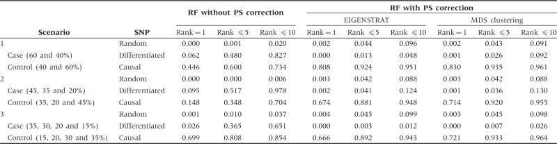 |
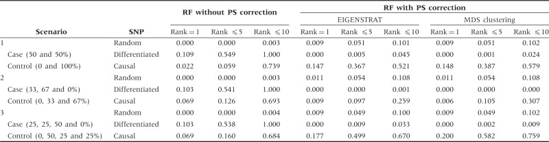
Table 2.
Proportions of SNPs with ranks of 1, ≤5 and ≤10 under extreme population stratification
 |
For each setting in different scenarios, we generate 1000 datasets. Each dataset consists of 10 000 SNPs for PS inference, 90 disease-unrelated random SNPs, 9 disease-unrelated differentiated SNPs and 1 causal SNP. The approach proposed by Price et al.15 is used to generate simulated SNPs. We assume that the Hardy–Weinberg equilibrium is valid for each SNP in each subpopulation. We generate 1000 cases and 1000 controls in each dataset. Details on the simulations of SNPs are given in the Supplementary data, available at IJE online.
Two additional simulations are performed under Scenarios 1–3 with moderate population stratification. The first one is performed to investigate whether the proposed method is robust to the selection of the GLM’s link function. A binary logistic model is fitted to remove the effect of PS from the phenotype. For the genotypes, we calculate the expected genotype for each SNP by P1 + 2P2, in which P1 and P2 are the probabilities of carrying one or two minor alleles predicted by a multinomial or ordinal logistic model. The corrected genotype is then defined by the difference between the observed and expected genotypes. The aim of the second one is to exclude the possibility that the correction effect is because of using IMSE instead of MDA. IMSE is used as the VIM for RF analysis without PS correction. The results are then compared with those obtained using MDA.
Evaluating performance
For each dataset, PS information is inferred using the 10 000 disease-unrelated SNPs. Association between the outcome and the 90 random SNPs, 9 differentiated SNPs and 1 causal SNP is then analysed by RF without and with correction for PS, respectively. We evaluate the performance of the proposed method based on either EIGENSTRAT or MDS clustering. As RF approach does not provide P-values as general hypothesis tests, it is not straightforward to derive measures for performance such as type I error rate and power in traditional methods. However, RF provides VIM for SNPs. Thus, for every simulated dataset in each scenario, we first obtain the permutation VIMs for all SNPs by RF. We use MDA for RF without PS correction and IMSE for RF with PS correction. SNPs are then sorted in descending order by VIM (MDA or IMSE) and ranked from 1 to 100. Ranks from the 1000 simulated datasets are then pooled by SNP types (random, differentiated and causal). As an example, for random SNPs, we will have 90 × 1000 ranks. For each of the three types of SNPs, we use histograms to compare the distributions of ranks between RF analyses without and with PS correction. We also calculate the proportions of SNPs with ranks of 1, ≤5 and ≤10.
Application to lactase (LCT)–height association
A spurious association between SNPs in the lactase (LCT) gene and height was reported by Campbell et al.23 It had been used to evaluate whether a correction method can remove the confounding effect of PS by several studies.24,25 We apply the proposed method to a GWAS dataset from the Harvard Lung Cancer Susceptibility Study. Details of participant recruitment for the study have been described previously.26 DNA was extracted from the whole blood and genotyped using the Illumina 610 k Quad chip. We restrict the analysis to 859 men with height information.
The original SNP reported by Campbell et al. is rs4988235. However, it is neither genotyped in the 610 k Quad chip nor imputed. We select to use two imputed SNPs, rs3754686 and rs2322660, which are both in high linkage disequilibrium (LD) with rs4988235 (r2 = 0.70 and 0.70, respectively). The imputation is performed using MaCH.27 The final dataset includes these two SNPs and other 998 randomly picked SNPs. RF analyses without and with PS correction are then performed using a dichotomized height (>175 and ≤175 cm) as the phenotype. An additional analysis is performed with a continuous height (cm) as the phenotype.
We use R statistical software (version 2.12) from R project (http://www.r-project.org/) for the simulation and statistical analysis. The R package ‘randomForest’ is used for RF analysis.28 For each forest, 1000 trees are grown. The number of SNPs sampled in each node is set to be 10 by default. Either the top 10 axes of variation (EIGENSTRAT) or the top 10 principal coordinates (MDS clustering) are included for PS correction.
Results
Correction for population stratification
Results from Scenarios 1–3 with moderate population stratification are presented in Table 1. The correction for PS improves the ability of identifying the causal SNP and decreases the ranks of differentiated SNPs when compared with the RF analysis without PS correction. For example, in Scenario 1, when PS is not corrected, the causal SNP is ranked the 1st in only 446 of the 1000 simulations, whereas the differentiated SNPs have the probability of 0.827 to present in the top 10 positions. After the PS correction, the probability to be ranked the 1st increases to 0.808 (EIGENSTRAT) or 0.830 (MDS clustering) for the causal SNP, and the differentiated SNPs only have a probability of 0.048 (EIGENSTRAT) or 0.092 (MDS clustering) to be ranked in the top 10 positions. We observe similar results from Scenarios 2 and 3.
The distributions of ranks generated in Scenario 1 with moderate population stratification are presented in Figure 1. It is not surprising that the distribution of differentiated SNPs is highly positively skewed if PS is not corrected (panel a), indicating a large possibility of being ‘falsely’ identified. We observe a decrease of importance for the differentiated SNPs and a consistent increase for the causal SNP after PS correction (panels b and c). Ranks from the random SNPs seem more likely to be uniformly distributed, except in the left tail. Results from Scenarios 2 and 3 (Supplementary Figures S1 and S2, available as Supplementary data at IJE online) follow similar patterns.
Figure 1.

Distributions of ranks of the three types of SNPs from Scenario 1 with moderate population stratification. The plots in panel (a) provide the distributions of ranks of VIMs from RF without PC correction. The plots in panels (b) and (c) give the distributions from RF with PS correction based on EIGENSTRAT and MDS clustering, respectively. In each plot, the x-axis is the rank of VIMs, ranging from 1 to 100, with 1 denoting ‘the most important’. The y-axis is the proportion of SNPs with rank equal to the coordinator in the x-axis
Results on exploring whether the correction will perform well under extreme mismatching of cases and controls are summarized in Table 2, as well as Supplementary Figures S3–S5 (available as Supplementary data at IJE online). For the highly differentiated SNPs, the possibility to be falsely identified as important SNPs is greatly increased if population stratification is not corrected, whereas the RF with PS correction achieves good correction. However, it should be noted that the PS correction also decreases the ability to identify the causal SNP, especially for Scenarios 1 and 2.
Correction for population admixture
Table 3 presents the results for applying the correction to simulated admixed populations. Once again, the RF with PS correction yields smaller VIMs for the differentiated SNPs than the RF without correction, and thus decreases the possibility of false discoveries. The corresponding distributions of ranks are provided in Figure 2 and Supplementary Figure S6 (available as Supplementary data at IJE online). RF with PS correction generates higher peaks for the causal SNP than the RF without correction.
Table 3.
Proportions of SNPs with ranks of 1, ≤5 and ≤10 under population admixture
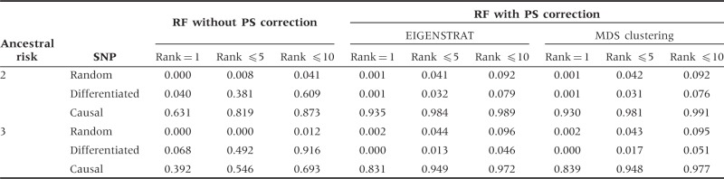 |
Figure 2.

Distributions of ranks of the three types of SNPs from Scenario 4 with an ancestral risk of 2
Comparison between EIGENSTRAT and MDS clustering
On eliminating false-positive results for disease-unrelated differentiated SNPs, EIGENSTRAT and MDS clustering have little difference in general. MDS clustering has better performance on increasing the importance of causal SNP than EIGENSTRAT, especially when the level of population stratification is extremely high.
Other characteristics of the proposed method
Simulations on evaluating whether the proposed correction is robust to the selection of GLM’s link function are performed by fitting a binary logistic model for phenotype and multinomial or ordinal logistic models for genotypes. By comparing the results (Supplementary Tables S2 and S3, available as Supplementary data at IJE online) with Table 1 (in which general linear model is used), we notice the difference is negligible, which indicates that the correction is robust to the selection of the GLM’s link function.
Supplementary Table S4 (available as Supplementary data at IJE online) presents the results of RF without PS correction but using IMSE as the VIM. It is worth noting that when the effect of PS is not corrected, the difference between RFs using MDA and IMSE as VIM is small in general, whereas a large improvement is observed on RF with PS correction. This provides the evidence that the correction effect of the proposed method is not related to VIM.
Correction for PS in the LCS–height dataset
Logistic regression analysis without correction for PS suggests that the two LCT SNPs, rs3754686 and rs2322660, are both associated with the dichotomized height (P = 1.05E-6 and 1.14E-5, respectively), indicating a possibility of PS. If the dichotomized height is used as the phenotype, the RF analysis without correction for PS shows that rs3754686 and rs2322660 are ranked the 1st and 2nd among the 1000 SNPs. After PS correction, their ranks are 551st and 443rd (EIGENSTRAT), or 156th and 252nd (MDS clustering). Similar result is observed when using the continuous height as the phenotype. The decreased importance of these two LCT SNPs indicates that the confounding effect of PS is removed from the RF analysis by the correction.
Discussion
In this article, we demonstrate that traditional RF approach may produce inaccurate result if the confounding effect of PS is not appropriately corrected in population-based association studies. When differentiated and causal SNPs are used to grow the forest simultaneously, they will ‘compete’ with each other to be selected to split the nodes. This competition may decrease the importance of the causal SNPs if the confounding effect of PS is strong. Although the axes of variation derived by EIGENSTRAT or the principal coordinates and cluster memberships derived by MDS clustering can be directly included in linear or logistic regression model for GWAS data analysis, our simulation results indicate that the correction effect is extremely limited when directly including the information of PS in the RF analysis as predictors (Supplementary Table S1, available as Supplementary data at IJE online). This may be because of the fact that the variables representing PS are not necessarily used as the root nodes of the trees, which limits the correction effect.
We propose a simple framework to correct the confounding effect of PS in RF analysis. The PS information is firstly extracted from a large number of SNPs by EIGENSTRAT or MDS clustering. The confounding effects are then removed from phenotype and genotypes by GLM. Our extensive simulation studies indicate that both EIGENSTRAT and MDS clustering work well under the framework of the proposed method, with MDS clustering having better performance. Li et al.25 proposed a phylogenetic approach to correct for PS by combining phylogeny constructed from SNPs and principal coordinates from MDS. They reported that the phylogenetic approach had better performance than MDS clustering for handling complex hierarchical PS. As the phylogenetic approach is an extension of EIGENSTRAT and MDS clustering, we believe it can also be applied in RF analysis under the proposed framework in principle. More studies are needed to verify this declaration.
The number of axes of variation or the principal coordinates to be adjusted is a possible concern in EIGENSTRAT analysis or MDS clustering. In our simulation, we use the top 10 axes for the inference of PS. We also study the sensitivity of the proposed method to the number of axes by using the top 20 axes from EIGENSTRAT for correction (not shown in this article). The results are almost identical to those using the top 10 axes. As the most extreme situation of population stratification in our simulations only includes four subpopulations, the proposed method is not sensitive to the number of axes used, given that the 10 axes are sufficient to capture the true feature of PS. In actual research, a Tracy–Widom test can be used to identify the appropriate number of axes to be used.29
In the simulation studies, the correction for PS results in a loss of efficiency when extreme case–control mismatching exists. This is in agreement with the reports by Price et al.15 and Li and Yu.17 As EIGENSTRAT analysis will ‘implicitly and automatically match cases and controls to extract the maximum possible amount of power from the data’,15 individuals failing to be matched would be ignored. As an example, for the extreme PS in Scenario 1, the adjusted analysis would only use the information from the 500 cases and 1000 controls in Population 2. Although MDS clustering has slightly better performance, we strongly recommend that carefully matching cases with controls on ancestry information should be used to achieve superior statistical power.
The confounding effect of PS is removed from both phenotype and genotypes. We observe through simulation that this provides stronger correction effect than the correction only on phenotype, especially for the disease-unrelated differentiated SNPs (Supplementary Table S5, available as Supplementary data at IJE online). Meanwhile, even though we prune the SNPs based on LD, two SNPs may still be indirectly correlated if both of them are correlated with the information of PS. As several studies have demonstrated that correlated predictors may bias the estimates of importance,6,30 we recommend removing the effect of PS from both phenotype and genotypes.
Genotype imputation provides the possibility for the scientists to evaluate the association at genetic markers that are not directly genotyped.31 In the analysis of the LCT–height-association dataset, rs3754686 and rs2322660, both imputed, are included in the analysis using the ‘best-guess’ genotypes. Some geneticists have suggested using the imputed allele dosages, which take values in [0,2], in the association analysis so as to account for uncertainty.32 We re-analyse the LCT–height dataset with a dichotomous height using all the SNPs in dosage format generated by MaCH. The result is similar to the one when the ‘best-guess’ genotypes are used (after correction for PS using EIGENSTRAT, rs3754686 and rs2322660 are ranked the 399th and 546th, respectively), which demonstrates that the proposed correction also works for the imputed GWAS data in dosage format.
We acknowledge this study has several limitations. First, although RF can be used to analyse GWAS data with thousands or even hundreds of thousands of markers, our simulation only uses 10 000 SNPs for the inference of PS information, and 100 SNPs for RF analysis. However, it has been reported that including too many non-informative SNPs in RF analysis will lower the overall signal-to-noise ratio and decrease the predictive ability of RF.7,10,33 Thus, an SNP-pruning procedure, based on LD, and feature selection are recommended before RF analysis. These will dramatically decrease the number of SNPs in the analysis and make our simulation a more likely realistic scenario. Second, it may not be straightforward to apply the proposed correction in RF analysis when the outcome is a categorical phenotype with more than two categories (multi-class outcome). A possible solution is to generate K binary indicator variables for each class of the phenotype (K is the number of classes of the outcome). RF analysis is then performed using each of the K indicator variables as the outcome, with correction for PS. As our approach has only been tested in a dataset with dichotomous and continuous outcomes, more studies are required to evaluate the performance of the proposed correction on RF analysis with multi-class outcome.
Supplementary Data
Supplementary Data are available at IJE online.
Funding
This work was supported by the National Cancer Institute of the U.S. National Institutes of Health (CA092824 to D.C.C.), the National Institute of Environmental Health Sciences of the U.S. National Institutes of Health (ES00002 to D.C.C.), and the National Natural Science Foundation of China (NSFC30901232 to Y.Z. and NSFC81072389 to F.C.).
Supplementary Material
Acknowledgements
The authors thank Dr Alkes Price for suggestions on simulations. They would also like to thank the reviewers for their comments and suggestions, which were very helpful for improving our manuscript.
Conflict of interest: None declared.
References
- 1.Thomas DC, Haile RW, Duggan D. Recent developments in genomewide association scans: a workshop summary and review. Am J Hum Genet. 2005;77:337–45. doi: 10.1086/432962. [DOI] [PMC free article] [PubMed] [Google Scholar]
- 2.McCarthy MI, Hirschhorn JN. Genome-wide association studies: past, present and future. Hum Mol Genet. 2008;17(R2):R100–01. doi: 10.1093/hmg/ddn298. [DOI] [PubMed] [Google Scholar]
- 3.Rosenberg NA, Huang L, Jewett EM, Szpiech ZA, Jankovic I, Boehnke M. Genome-wide association studies in diverse populations. Nat Rev Genet. 2010;11:356–66. doi: 10.1038/nrg2760. [DOI] [PMC free article] [PubMed] [Google Scholar]
- 4.Hirschhorn JN, Daly MJ. Genome-wide association studies for common diseases and complex traits. Nat Rev Genet. 2005;6:95–108. doi: 10.1038/nrg1521. [DOI] [PubMed] [Google Scholar]
- 5.Breiman L. Random forests. Mach Learn. 2001;45:5–32. [Google Scholar]
- 6.Nicodemus KK, Malley JD, Strobl C, Ziegler A. The behaviour of random forest permutation-based variable importance measures under predictor correlation. BMC Bioinformatics. 2010;11:110. doi: 10.1186/1471-2105-11-110. [DOI] [PMC free article] [PubMed] [Google Scholar]
- 7.Goldstein BA, Hubbard AE, Cutler A, Barcellos LF. An application of random forests to a genome-wide association dataset: methodological considerations & new findings. BMC Genet. 2010;11:49. doi: 10.1186/1471-2156-11-49. [DOI] [PMC free article] [PubMed] [Google Scholar]
- 8.Maenner MJ, Denlinger LC, Langton A, Meyers KJ, Engelman CD, Skinner HG. Detecting gene-by-smoking interactions in a genome-wide association study of early-onset coronary heart disease using random forests. BMC Proc. 2009;3(Suppl 7):S88. doi: 10.1186/1753-6561-3-s7-s88. [DOI] [PMC free article] [PubMed] [Google Scholar]
- 9.Kim Y, Wojciechowski R, Sung H, et al. Evaluation of random forests performance for genome-wide association studies in the presence of interaction effects. BMC Proc. 2009;3(Suppl 7):S64. doi: 10.1186/1753-6561-3-s7-s64. [DOI] [PMC free article] [PubMed] [Google Scholar]
- 10.Sun YV, Cai Z, Desai K, et al. Classification of rheumatoid arthritis status with candidate gene and genome-wide single-nucleotide polymorphisms using random forests. BMC Proc. 2007;1(Suppl 1):S62. doi: 10.1186/1753-6561-1-s1-s62. [DOI] [PMC free article] [PubMed] [Google Scholar]
- 11.Ziegler A, Konig IR, Thompson JR. Biostatistical aspects of genome-wide association studies. Biom J. 2008;50:8–28. doi: 10.1002/bimj.200710398. [DOI] [PubMed] [Google Scholar]
- 12.Lander ES, Schork NJ. Genetic dissection of complex traits. Science. 1994;265:2037–48. doi: 10.1126/science.8091226. [DOI] [PubMed] [Google Scholar]
- 13.Freedman ML, Reich D, Penney KL, et al. Assessing the impact of population stratification on genetic association studies. Nat Genet. 2004;36:388–93. doi: 10.1038/ng1333. [DOI] [PubMed] [Google Scholar]
- 14.Marchini J, Cardon LR, Phillips MS, Donnelly P. The effects of human population structure on large genetic association studies. Nat Genet. 2004;36:512–17. doi: 10.1038/ng1337. [DOI] [PubMed] [Google Scholar]
- 15.Price AL, Patterson NJ, Plenge RM, Weinblatt ME, Shadick NA, Reich D. Principal components analysis corrects for stratification in genome-wide association studies. Nat Genet. 2006;38:904–09. doi: 10.1038/ng1847. [DOI] [PubMed] [Google Scholar]
- 16.Price AL, Zaitlen NA, Reich D, Patterson N. New approaches to population stratification in genome-wide association studies. Nat Rev Genet. 2010;11:459–63. doi: 10.1038/nrg2813. [DOI] [PMC free article] [PubMed] [Google Scholar]
- 17.Li Q, Yu K. Improved correction for population stratification in genome-wide association studies by identifying hidden population structures. Genet Epidemiol. 2008;32:215–26. doi: 10.1002/gepi.20296. [DOI] [PubMed] [Google Scholar]
- 18.Sun YV. Multigenic modeling of complex disease by random forests. Adv Genet. 2010;72:73–99. doi: 10.1016/B978-0-12-380862-2.00004-7. [DOI] [PubMed] [Google Scholar]
- 19.Nicodemus KK, Malley JD. Predictor correlation impacts machine learning algorithms: implications for genomic studies. Bioinformatics. 2009;25:1884–90. doi: 10.1093/bioinformatics/btp331. [DOI] [PubMed] [Google Scholar]
- 20.Kaufman L, Rousseeuw PJ. Finding Groups in Data: An Introduction to Cluster Analysis. New York: Wiley Online Library; 1990. [Google Scholar]
- 21.Tibshirani R, Walther G, Hastie T. Estimating the number of clusters in a data set via the gap statistic. J R Stat Soc Series B Stat Methodol. 2001;63:411–23. [Google Scholar]
- 22.Rothman KJ, Greenland S, Lash TL. Modern Epidemiology. Philadelphia, PA: Lippincott Williams & Wilkins; 2008. [Google Scholar]
- 23.Campbell CD, Ogburn EL, Lunetta KL, et al. Demonstrating stratification in a European American population. Nat Genet. 2005;37:868–72. doi: 10.1038/ng1607. [DOI] [PubMed] [Google Scholar]
- 24.Qin H, Morris N, Kang SJ, et al. Interrogating local population structure for fine mapping in genome-wide association studies. Bioinformatics. 2010;26:2961–68. doi: 10.1093/bioinformatics/btq560. [DOI] [PMC free article] [PubMed] [Google Scholar]
- 25.Li M, Reilly MP, Rader DJ, Wang LS. Correcting population stratification in genetic association studies using a phylogenetic approach. Bioinformatics. 2010;26:798–806. doi: 10.1093/bioinformatics/btq025. [DOI] [PMC free article] [PubMed] [Google Scholar]
- 26.Asomaning K, Miller DP, Liu G, et al. Second hand smoke, age of exposure and lung cancer risk. Lung Cancer. 2008;61:13–20. doi: 10.1016/j.lungcan.2007.11.013. [DOI] [PMC free article] [PubMed] [Google Scholar]
- 27.Li Y, Willer CJ, Ding J, Scheet P, Abecasis GR. MaCH: using sequence and genotype data to estimate haplotypes and unobserved genotypes. Genet Epidemiol. 2010;34:816–34. doi: 10.1002/gepi.20533. [DOI] [PMC free article] [PubMed] [Google Scholar]
- 28.Liaw A, Wiener M. Classification and regression by randomForest. R News. 2002;2:18–22. [Google Scholar]
- 29.Patterson N, Price AL, Reich D. Population structure and eigenanalysis. PLoS Genet. 2006;2:e190. doi: 10.1371/journal.pgen.0020190. [DOI] [PMC free article] [PubMed] [Google Scholar]
- 30.Strobl C, Boulesteix AL, Kneib T, Augustin T, Zeileis A. Conditional variable importance for random forests. BMC Bioinformatics. 2008;9:307. doi: 10.1186/1471-2105-9-307. [DOI] [PMC free article] [PubMed] [Google Scholar]
- 31.Li Y, Willer C, Sanna S, Abecasis G. Genotype imputation. Annu Rev Genomics Hum Genet. 2009;10:387–406. doi: 10.1146/annurev.genom.9.081307.164242. [DOI] [PMC free article] [PubMed] [Google Scholar]
- 32.Zheng J, Li Y, Abecasis GR, Scheet P. A comparison of approaches to account for uncertainty in analysis of imputed genotypes. Genet Epidemiol. 2011;35:102–10. doi: 10.1002/gepi.20552. [DOI] [PMC free article] [PubMed] [Google Scholar]
- 33.Amaratunga D, Cabrera J, Lee YS. Enriched random forests. Bioinformatics. 2008;24:2010–14. doi: 10.1093/bioinformatics/btn356. [DOI] [PubMed] [Google Scholar]
Associated Data
This section collects any data citations, data availability statements, or supplementary materials included in this article.