Functional Network Changes in Hippocampal CA1 after Status Epilepticus Predict Spatial Memory Deficits in Rats

Abstract

Status epilepticus (SE) is a common neurological emergency, which has been associated with subsequent cognitive impairments. Neuronal death in hippocampal CA1 is thought to be an important mechanism of these impairments. However, it is also possible that functional interactions between surviving neurons are important. In this study we recorded in vivo single-unit activity in the CA1 hippocampal region of rats while they performed a spatial memory task. From these data we constructed functional networks describing pyramidal cell interactions. To build the networks, we used maximum entropy algorithms previously applied only to in vitro data. We show that several months following SE pyramidal neurons display excessive neuronal synchrony and less neuronal reactivation during rest compared with those in healthy controls. Both effects predict rat performance in a spatial memory task. These results provide a physiological mechanism for SE-induced cognitive impairment and highlight the importance of the systems-level perspective in investigating spatial cognition.

Introduction

Status epilepticus (SE), defined as an epileptic seizure lasting 30 or more minutes, is a common medical neurological emergency (DeLorenzo et al., 1996). It is associated with acute hippocampal injury (VanLandingham et al., 1998; Scott et al., 2002) and the later development of epilepsy, behavioral disruption, and cognitive impairment (Bourgeois et al., 1983; Jambaqué et al., 1993; Bailet and Turk, 2000). Potential mechanisms for these adverse outcomes include neuronal death (Sutula, 1991; Ben-Ari, 2001), abnormalities in synaptic transmission between interneurons and pyramidal cells (Lothman et al., 1995; Mangan et al., 1995; Morin et al., 1999), synaptic reorganization with mossy fiber sprouting (Sutula et al., 1989; Cavazos and Cross, 2006), and increased neurogenesis (Parent et al., 2006, 2008). While these physiological changes have been well documented, it is unknown whether these changes alter functional networks in the brain. It is possible that functional relationships between neurons are disrupted by SE and that these disruptions lead to adverse cognitive outcomes. Here we investigate this possibility.

Previous research linking neuronal activity and spatial memory in rats has focused on a subset of hippocampal pyramidal neurons called place cells. These cells discharge rapidly when a rodent enters a cell-specific location in the environment, or “firing field” (O'Keefe and Dostrovsky, 1971). Both individual place cell function and the interaction of place cell activity with theta oscillations predict spatial memory (O'Keefe and Recce, 1993; Lenck-Santini and Holmes, 2008).

Place cell activity also relates to spatial cognition through a phenomenon called replay. During replay, which occurs during sleep and wakeful inactivity, place cells recapitulate firing patterns observed during navigation (Skaggs and McNaughton, 1996; Foster and Wilson, 2006). This coordination of place cells, independent of the rat's physical location, is evidence of regulated functional connections between cells, i.e., a functional network. Disruption of this coordination may impair spatial memory (Ego-Stengel and Wilson, 2010). It is unknown whether replay is disrupted after SE and whether any disruption is associated with impaired spatial memory.

Here we examine the structure of functional networks in the CA1 region of SE and healthy rats. We analyze both place cells and nonplace pyramidal neurons. While ∼40% of pyramidal neurons in a given environment do not show place-dependent activity (Guzowski et al., 1999), these neurons are active suggesting a role in spatial navigation. We use global maximum entropy methods to construct networks of CA1 pyramidal neurons in rats performing a navigation task.

We investigate whether pilocarpine-induced SE changes the structure of these functional networks, and whether these changes are associated with deficits in spatial memory. We compare networks between the navigation and resting phases of the task to examine the extent to which functional interactions between neurons are reactivated during rest. We show that informative functional networks can be constructed between pyramidal cells in the CA1 region. SE networks are more synchronous and show significantly less replay than control networks. Both features strongly correlate with spatial memory providing a systems level mechanism for cognitive deficits in rats with pilocarpine-induced SE.

Materials and Methods

Rats.

Sprague Dawley male rats (300–350 g) were used in the study. All behavioral, pharmacological, and surgical procedures were done in accordance with National Institutes of Health guidelines and approved by the Dartmouth College Institutional Care and Use Committee.

Seizure induction.

The lithium-pilocarpine model was used for this study. The pilocarpine model of temporal lobe epilepsy is a commonly used rodent model of SE. In this model, the cholinomimetic convulsant pilocarpine is used to induce SE, which is followed by hippocampal damage and development of spontaneous recurrent seizures (Turski et al., 1983; Cavalheiro et al., 1991; Mello et al., 1993). The spontaneous temporal lobe seizures, cell loss, and synaptic reorganization that occur following pilocarpine-induced SE are similar in many respects to damage observed in human temporal lobe epilepsy (Mello et al., 1993). The use of lithium as a pretreatment before pilocarpine allows a reduction of the pilocarpine dose required to induce SE and results in a higher percentage of animals developing SE (Müller et al., 2009).

Following the initial acute seizures, there is a latent period of on average 2 weeks during which the rodents do not experience seizures. After this period, the animals begin to experience spontaneous seizures, averaging three per week. The spontaneous seizures are typified behaviorally by chewing motions, falling, head nodding, and forelimb clonus, while electrographically they are characterized by hippocampal discharges that spread to cortical regions (Leite et al, 1990; Cavalheiro et al., 1991).

In this study seizures were induced on postnatal day 60 (P60) as described by Cavalheiro et al. (1991). The control group received all drugs given to the experimental group except that they received saline instead of pilocarpine on P60.

Figure-8 maze.

All behavioral experiments were performed in a figure-8 maze. This maze consisted of a circular track 1 m in diameter with a center bridge connecting a feeder region to the wall on the opposite side of the maze (see Fig. 4). The walls were 60 cm high, and the arms were inclined 30° to allow the CCD camera an unobstructed view of the rat. In the feeder region a food dispenser (Lafayette Instruments) was placed on the outside wall of the maze. An experimenter in the adjacent room activated the food dispenser delivering a 20 mg sucrose pellet to a cup located on the inside wall of the maze.

Figure 4.

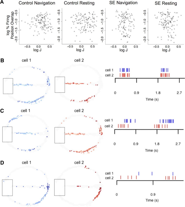
The relationship between spatial firing patterns and J. A, Correlations of spatial overlap in firing and J. Shown is the relationship between pairwise values of J and the pairwise overlap of spatial firing patterns. Each point represents one pair of neurons. There were no significant relationships between J and spatial overlap of neuronal firing. B–D, Example of spatial firing patterns for pairs of neurons with values of J that were (B) significantly positive (J = 2.7), (C) significantly negative (J = −1.3), and (D) not significantly different from 0. The left side shows the spatial firing pattern of each neuron in the pair. Note the overlap between fields in each pair. Feeding areas are outlined in black. The right side shows representative firing patterns for the neurons shown on the left to demonstrate how varying values of J can result from pairs of neurons with overlapping patterns of firing.

Behavioral training.

Training the rats to alternate directions in the maze consisted of four stages. Four days before the start of training, the rats were handled for 20 min per day and their food was restricted to achieve 85% ad libitum weight. The first stage of training was habituation. The rats were placed in the maze for 15 min twice per day and allowed to explore. During this phase 10 food pellets were placed in the reward cup. The second stage of training began after the rat had eaten all 10 pellets. In the second stage of training, the feeder was activated if the rat moved >50 cm from it, regardless of which direction the rat chose. The rat graduated to the third stage of training after it had received 10 food rewards during the second stage. In the third stage, a food pellet was awarded if the rat walked away from the feeder around the circle and returned via the center walkway. This stage took an average of 1 week to train. In the fourth and final stage of training, the rats were trained to alternate directions in the maze and return to the feeder through the center walkway.

Performance score.

During the memory task, each rat was required to alternate left and right turns in the maze and return to the feeder via the center walkway. A performance index (P_I) was calculated for each session based on how many of these turns the rat completed successfully. To calculate P_I we treated the rat's behavior in the navigation task as a Markov chain with three states, “left,” “right,” and “other.” In a perfect session the probabilities of transitioning from state left to state right and vice versa are both 1. To calculate the observed transition probabilities in each session, we constructed a 3 × 3 matrix to count the rat's transitions between each of the three states during its navigation session. The columns and rows of the matrix were labeled with the three possible states, left, right, and other. Each of the rat's decisions was tallied in this matrix. For example, if the rat turned left after a right turn the matrix entry indicating the transition from left to right was incremented by 1. After each turn was counted, this tally matrix was converted to a transition matrix by normalizing each row such that each summed to 1. We then calculated the distance between the ideal matrix and the actual matrix by subtracting the actual matrix from the ideal matrix and calculating the Frobenius norm of the resulting matrix. The Frobenius norm of an m × n matrix is the square root of the sum of the squares of its elements as seen in the following equation:

Because the Frobenius norm is a distance measure, rats that did more poorly, i.e., had transition matrices farther from the ideal transition matrix, had higher scores. To calculate a performance score that ranged between 0 and 1, with 1 being a perfect score, we normalized the Frobenius scores by dividing by the maximum Frobenius norm across all rats and then subtracted these values from 1.

Rats were observed for an hour before each testing session, and no sessions were used in which the rat had a seizure before or during the testing session.

Electrode array and implantation.

Single units in CA1 were recorded using a multi-electrode array manufactured in Robert U. Muller's Laboratory (State University of New York, Downstate Medical Center, Brooklyn, NY). The array had six independently drivable tetrodes and two 100 μm single wire electrodes that allowed differential recording above and below the CA1 pyramidal layer. The electrode tips were placed surgically in the dorsal CA1 region of the hippocampus at the following coordinates: anteroposterior: −3.8; lateral: −2; dorsoventral: −1.5 mm to bregma [(34)]. Rats were anesthetized with 1.5% halothane in 1 L/min of oxygen and placed in a stereotaxic frame. The skull was exposed and three anchor screws were placed over the left olfactory bulb, the right frontal cortex, and the right parietal cortex. A 2 mm hole was bored in the left parietal bone and the dura was removed to expose the brain surface. Electrode tips were then placed above CA1. Petroleum jelly was applied to the exposed brain surface and the electrode guide tube. Grip cement was applied to the skull, anchor screws, and around the electrode. Rats were allowed to recover for 4 d before screening for units began.

Data acquisition.

Before recording was begun, it was verified that each electrode of the implant was picking up waveforms of sufficient amplitude when the rat was resting in a 33 cm diameter cylinder. The electrodes were monitored twice a day and advanced 20 μm until ripples and unit activity from CA1 were observed. The electrodes were then advanced 10 μm or less once a day until one or more pyramidal cells with waveform amplitude >100 μV was isolated. Each cell or group of cells was recorded for one 15 min session in the figure-8 maze. To avoid recording the same cells twice, the electrodes were advanced 20 μm after each recording session. If a cell's place field and/or waveform looked similar to any observed on the preceding recording, it was discarded.

Unit discrimination.

Unit discrimination was done with cluster-cutting software (Cluster 3D, Neuralynx). Three aspects of the waveform were used to discriminate between pyramidal cells and interneurons: (1) the spike width, defined as the time separating the point of 25% amplitude before the peak and the time of minimum amplitude after the peak; (2) the most frequently occurring interspike interval (ISI), seen as the peak on the ISI histogram; and (3) the overall session firing rate. Pyramidal neurons typically fire rapidly in bursts in their place fields, but are silent elsewhere. During bursts, place cell ISI ranges between 5 and 8 ms. Because they are silent elsewhere in the maze, their overall firing rate is low. Thus pyramidal neurons were defined as neurons whose average spike width was >200 μs, whose most frequent ISI was lower than 8 ms, and whose overall session firing rate is <5 Hz. Interneurons do not burst, but fire relatively continuously and slowly compared with the pyramidal neuron bursts. These cells were defined as neurons whose spike width was <200 μs, whose most frequent ISI was >8 ms, and whose overall session firing rate was >5 Hz. Neurons that did not fit all criteria for one cell type or the other were not included in the analysis.

Network construction.

A network was built for each session using spike trains recorded during that session. Each network was built using entropy maximization, which is derived from statistical physics (Jaynes, 1957; Landau and Lifshitz, 1980).

Only those sessions in which at least 10 pyramidal neurons had been recorded simultaneously were used to build networks. Twelve sessions among four control rats and five sessions in three SE rats met this criterion. There was an average of 12 pyramidal cells per session in the controls and 15 pyramidal cells per session in the SE animals. There was no significant difference in the number of cells per network in controls and SE animals (Mann–Whitney U test, p = 0.3).

The data were binned into 30 ms windows (Fig. 1 Step 1). This time scale has previously been shown to be a physiologically relevant interval of synchrony between pyramidal cells in the hippocampus (Harris et al., 2003). For each neuron, bins in which at least one firing event occurred were labeled 1, and bins in which no firing occurred were labeled 0. This binning process resulted in a series of vectors of 0s and 1s representing the state of the network at each given time.

Figure 1.

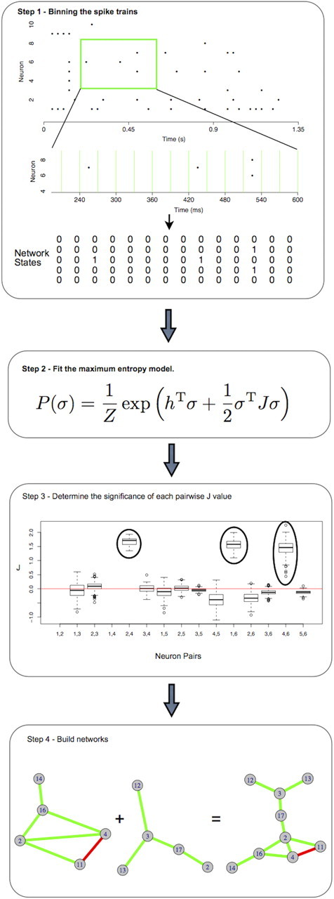
Schematic of network construction. Step 1, Spike trains were binned into 30 ms bins. Five nodes were randomly selected. Network states are represented by vectors of length five in which each neuron either fires (1) or does not fire (0). Step 2, Iterative scaling was used to fit mean firing rates and pairwise firing rates to the maximum entropy distribution. σ_1…σ_N are the states of neurons 1 through N, Z is a normalizing constant, h₁…h_N is the firing bias of neurons 1 through N, and J₁₂…J_N(N−1) is the propensity for each pair of neurons to fire together. This step is performed for 300 five-node networks for each session. Each network is resampled 1000 times. Step 3, The total variance in J produced by resampling for selected pairs of neurons. J was considered significant (circled values) if all estimates were on one side of 0. Step 4, Pairs of neurons with significant J values between them were linked together. Green connections represent positive values of J (synchrony) and red connections represent negative values of J (anti-correlated firing). Subsampled five-node networks from a single session were combined to form a single network. The networks shown are examples from the control group.

The bins were separated into two behavioral phases: navigation and resting. The rat was designated as resting when it entered the feeder region (see Fig. 4) and as navigating in all other areas of the maze. Due to computational constraints, we sampled five neurons at a time and used iterative scaling to maximize the entropy over all network states in this sample (Darroch and Ratcliff, 1972; Schneidman et al., 2006; Tang et al., 2008) (Fig. 1, Step 2). During the iteration process, we calculate the probability distribution over all states of the network (2^N), which increases exponentially with the number of nodes (N) in the network. Furthermore, the number of iterations required to converge on the precise model estimate increases with increasing network size. By limiting the sample size to five neurons we can calculate precise model estimates in a relatively short amount of time.

This subsampling process places neurons into different global contexts as they are grouped with different subsets of neurons in each sample. Consistent estimates of J across different subsampled networks support the hypothesis that J is driven by pairwise, rather than higher order, interactions. Context-independence of J allows us to merge subsampled networks into a single large network for each session while avoiding the enormous computational requirements of fitting the entire network at once. To estimate the variance in J across network subsamples, we sampled 300 five-node networks from each session. For each five-node network, we resampled the network states with replacement 1000 times and re-estimated J for each resampling of the states. We examined the variance in J that resulted from these resampling strategies.

Figure 1, Step 3 shows representative variance in estimates of J across the resampling conditions. The variance is low indicating that estimates of J for the entire network are reliably estimated by five-node subsamples. Interactions were considered significant if J was either positive or negative in all resamplings (Fig. 1, Step 3, circled values). To construct one network for each navigation session, links were placed between pairs of neurons for which a significant J had been calculated (Fig. 1, Step 4). These large networks were used for all subsequent analyses.

Calculating multi-information.

To determine how effective the pairwise maximum entropy model is at describing network behavior, we calculated a quantity called multi-information. Multi-information is the difference in Shannon entropy (S) between the independent model probability distribution (S_ind) and the observed probability distribution (S_obs). Shannon entropy is defined in terms of the probability of all states in the network as follows:

To estimate entropy, we use the NSB algorithm introduced in Nemenman et al. (2002). We use the MATLAB package described previously (Nemenman, 2011). This algorithm reduces the bias in entropy estimates for probability distributions in which the number of possible states exceeds the number of samples. This method has been shown to perform well on highly undersampled spike train data like the data used here (Nemenman et al., 2004).

The observed probability distribution, in a system of N neurons, takes into account all possible interactions from two-way up to N-way interactions. The entropy of this probability distribution is necessarily lower than the entropy of the independent model, which assumes no interactions between neurons. The gap in entropy between the independent and observed probability distributions is called multi-information. The closer the entropy of the maximum entropy model is to the observed model, the better it is at explaining the data. This proximity is expressed as a percentage of the multi-information explained by the maximum entropy model.

We calculated the proportion of the multi-information accounted for by the maximum entropy distribution (I_prop) for each five-node network as follows:

J and spatial information.

To investigate the possibility that J was related to spatial information, we examined whether values of J between each pair of neurons correlated with the overlap in their spatial firing patterns. Spatial patterns of cell firing were determined by analyzing video of rat performance during the navigation task. An in-house MATLAB script was used to calculate the X,Y position of the rat's head during each 30 ms time window during the task. The X,Y positions were aligned in time with neuronal firing information to determine the rat's head location at the time each neuron fired. The sets of unique X,Y points at which neurons 1 and 2 fired are P1 and P2, respectively. The spatial overlap of these two cells (O_1,2) was defined as the number of points shared between these sets divided by the number of total points in the two sets as follows:

This overlap was calculated independent of time, meaning the cells were not required to fire in the same time step to be considered overlapping in space. Pearson correlation was used to calculate the correlation between percentage overlap and the value of J for each pair of neurons in the session.

Calculating H_S.

Each network in this study represents a single navigation session of one rat. This network is associated with a single performance score and is composed of nodes of varying connectivity. To visualize the relationship between the connectivity of these nodes and performance, we constructed 2D histograms. In each histogram the x-axis represents performance divided into nine evenly spaced bins between 0 and 1. Each network falls along the x-axis according to its associated performance score. Each node in this network lies along the y-axis in accordance with its connectivity in the network (see Fig. 8).

Figure 8.

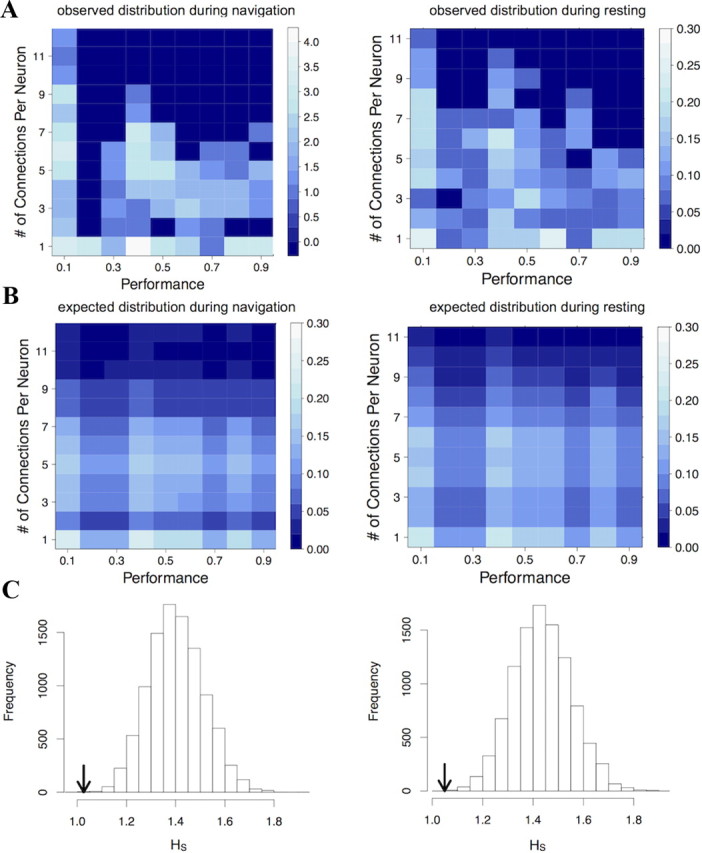
Correlation between performance and the number of connections per neuron in navigation and resting networks. A, 2D histograms show the observed relationship between connectivity distribution and performance for navigation (left) and resting (right) networks. Each cell shows the probability of observing a neuron with a given number of connections within a network matched with a particular performance. Lighter colors indicate higher probabilities. Networks of low performances tend to have highly connected neurons in them, while networks of high performances tend to have more poorly connected neurons. B, If there was no relationship between performance and the number of connections per neuron, we would expect this relationship to be much more evenly distributed. C, In comparing the observed value of H_S to the null distribution of expected values, we found that the observed values of H_S are extremely unlikely to have been measured by chance. This is true for both navigation (p = 1 × 10⁻⁴) and resting (p = 1 × 10⁻⁴). Arrows signify the observed H_S relative to the null distribution. These results indicate that high levels of synchrony, measured as high numbers of connections per neuron, predict poor spatial memory.

That the upper right quadrants of the 2D histograms have few entries suggests that highly connected nodes rarely occur in high-performing animals. We designed the statistic H_S to quantify this observation. H_S is a single number that quantifies the extent to which nodes fall into the upper right quadrant of the 2D histogram. H_S is calculated in the following way:

where P_i is the performance index associated with the nodes 1 through N in all networks in either the navigation or resting phase, and C_i is the connectivity of each node. Thus, H_S is large when highly connected nodes occur in high-performing networks and decreases monotonically as connectivity and performance decrease.

If highly connected nodes are disproportionately rare in high-performing animals, the observed H_S will be smaller than expected at random. To determine whether this is the case, we compared the observed values of H_S in the navigation and resting networks to their respective null distributions. We sampled the null distribution of H_S separately for the resting and navigation networks in the following way. We constructed a set of random networks by drawing with replacement from the connectivity distribution of the observed networks. Not all sequences of node connectivities can form a network. Thus, for each random draw of node connectivities, we checked that it was an admissible network sequence (Erdös and Gallai, 1960). We resampled the connectivity distribution until we had the same number of admissible networks as networks in the original group. This resampling procedure ensures that the null distribution of connectivities is drawn from the same distribution as the observed networks and is properly constrained. Next, we randomly assigned each performance index to one of the random networks and calculated H_S for this random population of networks and performance indices. In this manner we sampled the null distribution of H_S 10,000 times.

To calculate the relationship between performance and network stability each variable was first normalized using a Box-Cox transformation and a Pearson correlation was performed to assess the correlation between the resulting normally distributed variables.

Calculating B_E.

During unit discrimination, signals from cells recorded on a single electrode are separated computationally. Traditional spike-sorting methods may introduce bias into correlations estimated between cells recorded on a single electrode (Ventura and Gerkin, 2012). It is possible that contamination between clusters could artificially inflate the estimated coordination between cells. To investigate whether such electrode bias influenced our results, we developed the statistic B_E to quantify whether cells recorded on the same electrode were more likely to be significantly coordinated than cells recorded on different electrodes. B_E > 0 indicates that cells recorded on the same electrode are more likely to be significantly coordinated, while B_E < 0 indicates that cells recorded on different electrodes are more likely to be significantly coordinated. B_E was calculated for each session as follows: all pairs of cells recorded in the session were tabulated and divided into two groups—pairs recorded on the same electrode and pairs recorded on different electrodes. We then calculated the proportion of each group of pairs that were determined significantly coordinated by maximum entropy. P_S represents the proportion of cell pairs recorded on the same electrode that were significantly coordinated. P_D represents the proportion of cell pairs recorded on different electrodes that were significantly coordinated. B_E is the difference between two proportions as follows:

Within each group (i.e., control resting, control navigating, etc.), we calculated B_E for all networks.

We then compared this observed distribution for the group to the null distribution of B_E for the group. The null distribution of B_E is the distribution of B_E we expect if there is no relationship between whether two cells are considered significantly coordinated and whether they were recorded on the same electrode. To generate each null distribution of B_E we permuted the electrode labels randomly among the cells within in each network. We then recalculated B_E for all networks in the group. We repeated this resampling 200 times. This number of resamplings is sufficient to thoroughly sample the space given the small number of electrodes with usable cells in each session.

Statistical analysis.

For all comparisons of values between groups (i.e., rat performance, cell-firing rates, number of cells per network, and all network stability calculations), groups were found to be non-normally distributed so Mann–Whitney U tests were performed to assess differences.

Pearson correlation was used to compare the relationship between J values and spatial firing patterns, as both variables had high n and were found to be approximately normally distributed.

To assess the difference in connectivity distribution between control and SE animals we used generalized estimating equations with an adjustment for connectivity within session. This approach was used rather than Pearson correlation because the observations of node connectivity within a session are not independent of each other. Similarly, parametric methods cannot be used to assess the relationship between node connectivity and performance because of the constraints placed on the distribution of each variable. Within a single network, the connectivities of individual nodes are not independent of each other. Furthermore a single network (containing nodes with different connectivities) is paired with a single performance score, further constraining the relationship between connectivity and performance. To address these constraints, we developed a statistic H_S (described above) that could be used to compare the observed distributions to null distributions.

Results

Rat behavior

We generated two groups of rats; the first underwent 90 min of pilocarpine-induced SE at least 2 weeks before being studied. Control rats were handled identically but were injected with saline rather than pilocarpine. The single-unit firing data were collected from rats performing a spatial navigation task in a figure-8 maze. The task was to alternate left and right turns through the maze and return to a feeder region for a food reward via a central bridge. Recordings from navigation sessions were selected for further analysis based on the following two criteria: (1) there were at least 10 pyramidal neurons recorded simultaneously and (2) the rat performed at least one turn correctly during the navigation task. Based on these criteria, we identified 12 sessions performed by four control rats and five sessions performed by three SE rats. Performance was not binary (correct vs incorrect) since there are many ways to run the maze incorrectly. For instance, even after choosing the correct direction out of the feeder region, a rat may have turned around in the circular arm to come back to the feeder region or traveled fully around the maze without returning via the straight segment. On average the controls had a performance index P_I = 0.45 95% confidence interval (CI): 0.35–0.59 (see Materials and Methods for calculation of performance score). SE rats performed significantly more poorly (P_I = 0.21, 95% CI: 0.11–0.31) confirming that rats exposed to pilocarpine-induced SE are impaired in spatial cognition.

Histology

Cell loss in three regions of the hippocampus (CA1, CA3, and the hilus of the dentate gyrus, DG) was scored using methods previously described (Shatskikh et al., 2009). Considerable cell loss was noted in the SE rats in three regions of the hippocampus (CA3, Cont. = 0.17 ± 0.17; SE = 2.67 ± 0.21; CA1, Cont. = 0.17 ± 0.17; SE = 2.53 ± 0.231; DG, Cont. = 0.17 ± 0.17; SE = 2.80 ± 0.20 p < 0.01, a Mann–Whitney statistic was used for each region). The results demonstrate that there was substantial cell loss in all three regions of the hippocampus, including CA1, which was the focus of our electrophysiological studies. Despite this we were able to record sufficient pyramidal cells in both groups for functional network analyses.

Evaluation of the pairwise entropy model

Before evaluating the characteristics of the functional networks it is essential to determine whether the pairwise maximum entropy model is sufficient to describe complex firing patterns in the CA1 hippocampal region. To build the models, spike trains from all pyramidal neurons recorded in each session were split into two epochs, navigation and rest. The rat was said to be resting when it entered the feeder region (see Fig. 4) and navigating in all other areas of the maze. The spike trains recorded during the session were binned into 30 ms bins (see Materials and Methods). For each neuron, bins in which at least one firing event occurred were labeled 1 and bins in which no firing occurred were labeled 0. This binning process resulted in a series of vectors of 0s and 1s representing the state of the network at each given time. A state of 01001, for example, indicates that in this 30 ms time window, neurons 2 and 5 fired while all other neurons remained silent.

The pairwise maximum entropy model uses information from direct pairwise interactions to predict the frequency of each of the network states exhibited by the recorded neurons. To evaluate the model performance, we compared the observed frequency of each network state to those predicted by the independent and maximum entropy models (Fig. 2). The pairwise maximum entropy model showed a marked improvement over the independent model in predicting the frequency of both common and rare network states.

Figure 2.

Evaluation of the second-order maximum entropy model. This plot shows the frequency of all network states predicted by both the independent model (green) and the pairwise maximum entropy model (blue) for all five-node networks sampled from all spike trains. Each point represents a single state of the network. All networks are plotted here. The line of equality (black) shows where the log of the empirical probability of a given state equals the log of the probability predicted by the model. States whose predicted probability was 0 do not appear on the plot because the log of 0 is undefined. The blue dots are less variable around the line confirming that the second-order maximum entropy model is a better predictor of observed state frequencies than the independent model.

To test how much of the total network behavior is explained by pairwise interactions, we used a quantity called multi-information (I_N), defined as the difference in Shannon entropy (S) between the independent model probability distribution (S_ind) and the observed probability distribution (S_obs) (see Materials and Methods). We found that, on average, 95% of the multi-information was accounted for in the controls and 92% was accounted for in the SE animals. Similar percentages were found in the second-order maximum entropy model in the cortex and retina ex vivo (Schneidman et al., 2006; Shlens et al., 2006; Tang et al., 2008). These results indicate that the pairwise maximum entropy model is a substantial improvement over the independent model in describing network behavior and that higher order interactions do not need to be calculated. On this basis we then built separate functional networks from data collected during navigation and rest.

The interpretation of neuronal interactions

From a biological perspective, the second-order maximum entropy model indicates which pairwise neuronal interactions, represented by the parameter J, are critical to the behavior of the overall network. It is important to note that these values of J do not represent physical, but rather functional interactions between pyramidal neurons. J is a statistical parameter relating the firing patterns of pairs of neurons. However, unlike a standard Pearson correlation, the maximum-entropy model takes network effects into account and can separate statistically direct relationships between neurons from network-mediated relationships (Fig. 3). A statistically direct connection between two neurons means that after the correlations with all other neurons in the model have been accounted for, there remains a statistical dependence between the two neurons under scrutiny. In this way J is analogous to a partial correlation in the continuous case. Because maximum entropy methods can discern direct from indirect statistical dependencies, functional networks built with this method are less influenced by false positive and false negative correlations than networks built with Pearson correlation coefficients. Figure 5 shows the relationship between J and Pearson correlation in the present data. It can be seen that although J and Pearson correlation are positively related, they are not identical. The results from Figures 3 and 5 together indicate that maximum entropy techniques yield a more reliable network than the simpler Pearson correlation.

Figure 3.

Maximum entropy methods can distinguish direct from network-mediated effects. In the upper cross-correlogram neurons A and B can be seen to have positively correlated firing (C_AB refers to the Pearson correlation coefficient between cells A and B. Here C_AB = 0.11). However, through entropy maximization (upper right) it can be deduced that this correlation is an artifact of neurons A and B interacting positively with neuron C (J_AC = 0.99, J_BC = 2.24). These results indicate that the interaction between neurons A and B is mediated through the network, not directly between neurons. Bottom, The cross-correlogram shows no functional relationship between neurons A and B (Pearson correlation C_AB = −0.002). However, through entropy maximization we find that these neurons are interacting positively (J_AB = 1.9). A positive interaction between neurons B and C (J_BC = 2.0) and a negative interaction between neurons A and C (J_AC = −0.6) cancel out any correlation that is visible on a cross-correlogram. These examples were drawn from the control rat networks. They show the importance of using global maximum entropy methods rather than local method like Pearson correlation for inferring direct relationships between neurons.

Figure 5.

Pearson Correlation versus J. The relationship between the Pearson correlation coefficient and J for pairs of neurons is positive, but nonlinear. All pairs of neurons across the controls and SE groups for both navigating and resting networks are presented here. Together with Figure 4, this indicates that maximum entropy methods are preferable to simple Pearson correlation in constructing functional networks between pyramidal neurons. The vertical and horizontal lines mark 0 to highlight the relationship between J and the Pearson correlation coefficient above and below 0. The large number of values of J at 0 are those that were not deemed significantly different from 0. This shows the range over which Pearson correlations can vary and not represent direct statistical interactions.

In the CA1 hippocampal region, pyramidal neurons do not directly synapse onto one another, but their activity can still be coordinated by other brain regions (e.g., entorhinal cortex, DG, and CA3). Neurons can fire together (J significantly > 0), at different times (J significantly < 0), or independently of one another (J not significantly different from 0). In both SE and control animals the values of J ranged from negative to positive during both navigation and resting. The presence of these interactions suggests that there is coordination of neuronal firing in CA1, even in the absence of physical connections between the pyramidal neurons.

As many pyramidal cells in hippocampal CA1 are place cells, it is possible that a positive J between two neurons simply indicates that these neurons have spatially overlapping firing patterns. To investigate this possibility we measured the correlation between the J of each neuron pair and the amount of spatial overlap in their firing (see Materials and Methods). We found that there was no correlation between J and spatial overlap of firing in either SE or control animals during navigation (Fig. 4A). A more detailed examination of neuronal firing patterns shows how this is possible (Fig. 4B–D). Neurons that fire in the same region of the maze may fire synchronously (Fig. 4B), offset (Fig. 4C), or independently of one another (Fig. 4D). These results show that the interactions between place cells include more than spatial relationships. Furthermore, nonplace neurons have significant interactions between them and with place cells indicating that they contribute to the structure of the functional network in CA1. Therefore, the networks were built using data from all pyramidal cells, including place cells and nonplace pyramidal neurons.

It is important to note that although, as shown in Figure 4, positive J corresponds to correlated firing and negative J corresponds to anti-correlated firing between two neurons, the precise nature of this correlation cannot be captured by Pearson correlation coefficients (Fig.5). The Pearson correlation between two neurons is influenced by other neurons in the network whereas J reflects the statistical dependency between two neurons after the influence of other neurons has been accounted for.

SE rats show higher neuronal synchrony than controls during both navigation and resting

Using the J calculated for each pair of neurons, we built a network for the neurons recorded in each session. We first asked whether there was a difference in overall network connectivity between SE and control animals. Connectivity between neurons indicates direct functional interactions between them. Neurons in these networks could fire highly synchronously (J significantly > 0), highly asynchronously (J significantly < 0), or independently of one another (J not significantly different from 0).

To quantify overall neuronal interaction in the rats, we calculated the number of connections made by each neuron and the sign of each connection (see Materials and Methods). There were a total of 241 neurons in the networks of all six animals (168 in controls and 73 in SE). We found that, during both navigation and rest, the average number of connections per neuron in SE rats (navigation = 4.41, 95% CI: 3.2–5.8; resting = 4.44, 95% CI: 3.7–5.2) was higher than that of control animals (navigation = 2.76, 95% CI: 2.0–3.0; resting = 2.76, 95% CI: 2.0–3.5) (navigation: p ≤ 0.001, resting: p = 0.005) (Fig. 6A,B). We also examined whether this difference was due to differences in the distribution of positive connections (J > 0) or negative connections (J < 0). We found that in both navigation and rest, the average number of positive connections per neuron was higher in SE animals (navigation = 4.72, rest = 4.41) than in control animals (navigation = 3.62, rest = 3.13) (navigation: p = 2.7 × 10⁻⁵, rest: p = 3.98 × 10⁻⁶) (Fig. 6C,D). The number of negative connections per neuron in the navigation network were not significantly different between SE (0.38) and control networks (0.30) (p = 0.47). During rest, the average number of negative connections per neuron in the SE networks (0.21) was lower than in the control networks (0.52) (p = 2.68 × 10⁻³). Differences in connectivity distributions remained significant after adjusting for the number of nodes in each network. Thus surviving pyramidal neurons are excessively synchronous and the neurons are more likely to fire together in the SE animals.

Figure 6.

Comparison of the number of connections per neuron in networks from control and SE rats. A, During navigation neurons in SE animals had significantly more connections (mean = 4.41 connections per neuron, 95% CI: 3.2–5.8) than neurons in control animals (mean = 2.76 connections per neuron, 95% CI: 2.0–3.0) (p < 0.001). B, This was also the case during resting. Neurons in SE animals had significantly more connections (mean = 4.44 connections per neuron, 95% CI: 3.7–5.2) than neurons in control animals (mean = 2.76 connections per neuron, 95% CI: 2.0–3.5) (p = 0.005). C, These connections were mostly positive, indicating a high degree of synchronous activity. During navigation neurons in SE animals had more positive connections (mean = 4.41 positive connections per neuron) than neurons in control animals (mean = 3.13 positive connections per neuron) (p = 0.002). D, This was also true during resting. In SE animals neurons had more positive connections to other neurons (mean = 4.51 positive connections per neuron) than neurons in control animals (mean = 3.09 positive connections per neuron) (p < 0.001). Large numbers of positive connections in SE networks indicate that, during both navigation and resting, CA1 pyramidal neurons in SE animals fire more synchronously than those in control animals.

To investigate the possibility that the higher number of connections per neuron in SE networks was an artifact resulting from more firing overall, we examined the rates of neuronal firing in controls and SE rats during both navigation and rest. The median overall firing rate per cell during the navigation phase in controls (0.75 Hz per cell) was not significantly different from the median overall firing rate in the SE animals (0.9 Hz per cell) (Mann–Whitney U p = 0.27). Similarly during resting the median firing rate per cell in controls (0.75 Hz) was not significantly different from that in SE rats (0.78 Hz) (Mann–Whitney U p = 0.15).

We also investigated whether there were artifacts from the neurological recordings that could contribute to the elevated synchrony observed in SE animals. During the recording process each electrode implanted in the rat's brain records signals from multiple cells. These signals are separated computationally. Although rigorous spike-sorting techniques were used, it is possible that signals from cells recorded on a single electrode may not be separated completely thereby increasing the likelihood that the cells are erroneously significantly coordinated by the maximum entropy method. Recently Ventura and Gerkin (2012) showed that correlations between bursty cells, like the place cells used here, may be overestimated if misclassification of spikes is high. Here we refer to this phenomenon as electrode bias. Such bias could artificially inflate the density of networks in this study. Further, if the SE group contains more cell pairs recorded on a single electrode than the control group, the increased connectivity in the SE group could be artifactual.

To investigate whether electrode bias influenced our results we first examined the extent to which electrode bias existed in our data. We quantified the bias of each network with the statistic B_E (see Materials and Methods). B_E > 0 indicates that cells recorded on the same electrode are more likely to be significantly coordinated, while B_E < 0 indicates that cells recorded on different electrodes are more likely to be significantly coordinated. We determined the amount of electrode bias in each group (i.e., control resting, control navigating, etc.) by calculating B_E for each network in the group and comparing the resulting distribution to the null distribution of B_E for that group (Fig. 7). The null distribution of B_E is the distribution we expect to see if there is no relationship between the likelihood that two cells are significantly coordinated and whether they were recorded on the same electrode.

Figure 7.

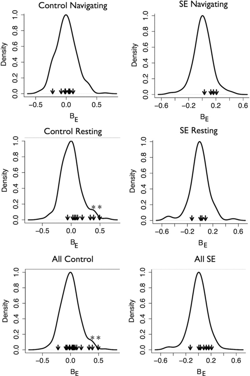
Comparisons of empirical values of probe bias to the null distribution in each subset of networks. Each panel shows the null distribution of B_E for the group (solid line) with the B_E value of each network in the group represented as arrows. Asterisks indicate the networks that are significantly biased. The p values of each K-S is as follows: Control Navigating: p = 0.84; SE Navigating: p = 0.1; Control Resting: p = 0.014; SE Resting: p = 0.78; All Control: p = 0.12; All SE: p = 0.15. These p values indicate that the only significant electrode bias is in the Control Resting group. Removing the significantly biased networks in this group does not affect the results in this paper, and cell pairs recorded on the same electrode are evenly distributed between SE and control groups. Together these results indicate very little possibility for electrode bias to affect the results reported here.

We used the two-sample Kolmogorov–Smirnov (K-S) test to determine whether the empirical values of B_E for each group were drawn from their respective null distributions. In all groups except for control resting, we accepted the null hypothesis that the samples were drawn from the null distribution (Fig. 7) and therefore there is no significant electrode bias. In the control resting group there were two significantly biased networks with high values of B_E. The 95% CIs of B_E for these two networks did not include 0 indicating that neuron pairs recorded on the same electrode were more likely to be significantly coordinated. The K-S test is sensitive to outliers and we suspect that these outlier networks were responsible for the overall rejection of the null hypothesis for this group. The presence of these networks in controls overall (“all control” group) did not lead to rejection of the null hypothesis, however, perhaps because of the high number of networks in this group. We investigated whether these two networks affected the results reported in this paper by removing them and recalculating all statistics. None of the results were affected by the removal of these networks indicating that the results reported here are unaffected by electrode bias.

We further investigated whether electrode bias was controlled for between the SE and control groups. If the proportion of cell pairs recorded on a single electrode is distributed evenly across groups, any existing electrode bias is controlled for. We used generalized estimating equations to estimate the uniformity of this distribution within individual sessions. The proportion of cells recorded on the same electrode was not distributed unevenly in either the resting networks (p = 0.33) or the navigating networks (p = 0.92).

In summary, only two networks in one group showed significant electrode bias. The removal of these networks does not affect the results reported here, and cell pairs recorded on a single electrode are evenly distributed across SE and control groups. Together, these results show that electrode bias is not a significant factor in this analysis.

After accounting for all potential biases, we found that the SE rats had more highly connected networks than controls, and because this group also performed more poorly in the navigation task, we investigated whether there was a correlation between performance in the maze and number of connections per neuron in the networks. Figure 8A shows the distribution of connections per neuron for each network associated with each performance score. Because observations of the number of connections for individual neurons are not independent of each other, we could not use a standard Pearson correlation on these data. Instead we constructed a statistic (H_S) to calculate the degree to which highly connected nodes were associated with high performance (see Materials and Methods). We compared the empirical statistic to a null distribution generated by resampling performance scores and the number of connections per neuron for each network. We calculated a null distribution for both navigation and resting networks (Fig. 8B). In both navigation and resting the observed H_S was significantly different from the mean of the null distribution (Fig. 8C) (navigation: p = 1 × 10⁻⁴; resting: p = 1 × 10⁻⁴). This shows that increased synchrony between pyramidal cells, during both navigation and rest, is significantly associated with decreased performance in the maze. This relationship remained significant after normalizing connectivity by the number of nodes in each network (navigation: p < 1 × 10⁻⁴; resting: p < 1 × 10⁻⁴).

SE rats show less replay in resting than controls

In addition to comparing networks between SE and control animals, we compared the networks generated during navigation and rest within each animal. The previously observed phenomenon of place cell replay suggests that neurons that are correlated during navigation will continue to be correlated during rest. We hypothesized that replay is disrupted in SE rats, and as a consequence, these rats would maintain fewer neuronal interactions between navigation and rest than control animals. We further hypothesized that because replay is known to be important to memory consolidation (Ego-Stengel and Wilson, 2010), high-performing animals would maintain correlated pairs of neurons at a higher rate than low-performing animals.

To quantify the stability of neuronal interactions between navigation and rest, we counted the pairs of neurons that were significantly correlated in both phases within a single maze-navigation session. To be considered maintained, the interaction was required to be significant and of the same sign (positive or negative) in both phases.

We quantified three aspects of interaction maintenance. First we examined the proportion of all pairs of neurons that maintained coordination between navigation and rest. We found that 15% of neuron pairs (100 pairs) in control animals maintained coordination, while in SE animals only 6% of neuron pairs (26 pairs) maintained coordination between the phases. This difference was significant (Mann–Whitney U p = 0.036) (Fig. 9A). The percentage of coordinated pairs was significantly correlated with performance in the maze (Pearson correlation R² = 0.39, p = 0.0077) (Fig. 9B).

Figure 9.

Comparison of replay in SE and control animals. These plots show the proportion of pairwise neuronal interactions that are retained between navigation and resting networks in each animal. A, Between navigation and resting control animals retain a significantly higher proportion of pairwise neuronal interactions (100 connections, 15%) than SE animals (26 connections, 6%) (Mann–Whitney U connections p = 6.07 × 10⁻³; proportions p = 0.04). This suggests that interactions between neurons established during navigation are reactivated during rest. B, The proportion of retained interactions correlates positively and significantly with performance (Pearson correlation R² = 0.39, p = 7.7 × 10⁻²) supporting previous work showing that replay is critical to spatial memory. C, The proportion of interactions formed during rest and retained during navigation was significantly different between SE (100 connections, 28%) and control (32 connections, 15%) animals (Mann–Whitney U connections p = 3.23 × 10⁻³; proportions p = 1.3 × 10⁻³). D, Retaining neuronal interactions from rest to navigation did not significantly affect performance (R² = 0.01, p = 0.7). E, The proportion of interactions formed during navigation and maintained during rest was significantly different between SE (99 connections, 31%) and control (34 connections, 15%) animals (Mann–Whitney U connections p = 3.23 × 10⁻³; proportion p = 3.23 × 10⁻³). F, The proportion of interactions retained from navigation to resting was also significantly correlated with performance (Pearson rank correlation R² = 0.41, p = 5.5 × 10⁻³). Together these results indicate that reactivation of functional networks is disrupted in SE animals and that this disruption affects spatial memory. x and y variables have been normalized to enable linear statistics.

Second we investigated whether there was directionality in the maintenance of coordination. We asked what proportion of coordinated neuron pairs in the navigation phase was retained during resting (Fig. 9C). We also asked what proportion of coordinated neuron pairs measured in the resting phase was retained during navigation (Fig. 9E). In control animals 28% (100 pairs) of the coordinated neuron pairs observed during navigation were maintained during rest. This figure was significantly different from that seen in the SE animals (15%, 32 pairs) (Mann–Whitney U p = 3.2 × 10⁻⁴). There was, however, no significant correlation between the proportion of coordinated neuron pairs retained from rest to navigation and performance in the maze (R² = 0.01, p = 0.7) (Fig. 9D).

On the other hand, when we examined the maintenance of coordinated neuron pairs from navigation to rest, we did see a significant correlation with performance. Control animals maintained a significantly higher proportion of coordinated neurons than SE animals between navigation and rest [control: 31% (99 pairs), SE: 15% (34 pairs)] (Mann–Whitney U p = 1.3 × 10⁻³) (Fig. 9E). Furthermore, across all animals there was a significant correlation between the proportion of neuron pairs retained and performance in the maze (Pearson rank correlation R² = 0.41, p = 5.5 × 10⁻³) (Fig. 9F).

To ensure that electrode bias did not influence these results, we recomputed each statistic after removing all cell pairs recorded on the same electrode. All significant differences and correlations remained significant.

Together these results support the hypothesis that replay is essential to spatial memory. Here we show for the first time that replay is disrupted in epileptic animals, and that this disruption is correlated with spatial memory. It is also important to note that within the controls, but not the epileptic animals, there is a relationship between maintenance of neuronal coordination between navigation and rest and performance.

Discussion

In the current study we show in a murine model that hippocampal CA1 pyramidal neurons operate in functional networks. Networks in animals exposed to pilocarpine-induced SE are more synchronized than those in control animals. We have also shown for the first time that replay is disrupted in epileptic animals. While it has been theorized that synchrony and replay have important roles in normal cognitive function, we demonstrate that in a disease state alterations in synchrony and replay predict impaired spatial memory.

The second-order maximum entropy model was used to assess the structure of functional networks. Although previously used in vitro and ex vivo (Schneidman et al., 2006; Shlens et al., 2006; Tang et al., 2008), the method had not been applied in vivo. Our evaluation of this model shows that, similar to previous work (Schneidman et al., 2006; Shlens et al., 2006; Tang et al., 2008), the second-order maximum entropy model explains the vast majority of the multi-information in the CA1 region. These results suggest that the statistical dynamics of neuronal networks in general may be captured by pairwise interactions. Such a universal feature is critically important to the study of these networks. As the size of a network grows, analysis of three-way, four-way, and higher order interactions rapidly becomes computationally intractable. If, as this and other studies suggest, the majority of neuronal network dynamics can be described using only pairwise interactions, the study of these networks is far more tractable than previously thought.

There are many potential causes of the network disruptions identified in this study. Many physiological and biochemical changes resulting from epilepsy have been documented in the hippocampus (Sutula, 1991, 1989; Lothman et al., 1995; Mangan et al., 1995; Mangan and Lothman, 1996; VanLandingham et al., 1998; Morin et al., 1999; Ben-Ari, 2001; Scott et al., 2002, 2003; Cavazos and Cross, 2006; Parent et al., 2006, 2008), and any of these could disrupt neuronal coordination. Changes in CA1 itself or in regions that regulate CA1, such as CA3 and the entorhinal cortex, could contribute to changes in the functional network of CA1. It is important to note that individual physiological and morphological changes to the hippocampus following SE may not correlate with cognitive deficits in epileptic rats. However, in concert these changes affect the overall behavior of the hippocampal functional network in a way that relates directly to rat behavior. Through a systems approach these effects become visible. Such a link to behavior suggests that systems methods, like the maximum entropy techniques used here, may be useful in developing biomarkers of cognitive impairment in epilepsy. Such biomarkers could help elucidate the impact of drugs and behavioral therapies on functional network structure in the hippocampus.

The results of this study show the potential of analyzing functional neuronal network structure in vivo from a clinically relevant and global perspective. We were able to detect relevant and significant differences between control and SE rats from in vivo recordings. Our results also indicate that pyramidal cells that are nonplace cells may be important in these networks, and therefore in spatial navigation. Future studies using more electrodes and longer recordings may be able to analyze a larger number of neurons in a single network. In larger ensembles it may be possible to analyze the effects of interneurons on these networks. Interneurons are the regulatory hubs in CA1, and as such may hold important network information. While the networks used here were too small to specifically address the contribution of nonplace cells to CA1 functional networks, future work with larger networks may also be able to examine the contribution of these cells in detail. Finally, it is possible that such a systems level approach my lead to therapies that specifically target systems-wide network disruptions.

References

- Bailet LL, Turk WR. The impact of childhood epilepsy on neurocognitive and behavioral performance: a prospective longitudinal study. Epilepsia. 2000;41:426–431. doi: 10.1111/j.1528-1157.2000.tb00184.x. [DOI] [PubMed] [Google Scholar]
- Ben-Ari Y. Cell death and synaptic reorganizations produced by seizures. Epilepsia. 2001;42(Suppl 3):5–7. doi: 10.1046/j.1528-1157.2001.042suppl.3005.x. [DOI] [PubMed] [Google Scholar]
- Bourgeois BF, Prensky AL, Palkes HS, Talent BK, Busch SG. Intelligence in epilepsy: a prospective study in children. Ann Neurol. 1983;14:438–444. doi: 10.1002/ana.410140407. [DOI] [PubMed] [Google Scholar]
- Cavalheiro EA, Leite JP, Bortolotto ZA, Turski WA, Ikonomidou C, Turski L. Long-term effects of pilocarpine in rats: structural damage of the brain triggers kindling and spontaneous recurrent seizures. Epilepsia. 1991;32:778–782. doi: 10.1111/j.1528-1157.1991.tb05533.x. [DOI] [PubMed] [Google Scholar]
- Cavazos JE, Cross DJ. The role of synaptic reorganization in mesial temporal lobe epilepsy. Epilepsy Behav. 2006;8:483–493. doi: 10.1016/j.yebeh.2006.01.011. [DOI] [PMC free article] [PubMed] [Google Scholar]
- Darroch J, Ratcliff D. Generalized iterative scaling for log-linear models. Ann Math Stat. 1972;43:1470–1480. [Google Scholar]
- DeLorenzo RJ, Hauser WA, Towne AR, Boggs JG, Pellock JM, Penberthy L, Garnett L, Fortner CA, Ko D. A prospective, population-based epidemiologic study of status epilepticus in Richmond, Virginia. Neurology. 1996;46:1029–1035. doi: 10.1212/wnl.46.4.1029. [DOI] [PubMed] [Google Scholar]
- Ego-Stengel V, Wilson MA. Disruption of ripple-associated hippocampal activity during rest impairs spatial learning in the rat. Hippocampus. 2010;20:1–10. doi: 10.1002/hipo.20707. [DOI] [PMC free article] [PubMed] [Google Scholar]
- Erdös P, Gallai T. Gráfok elümloírt fokszámú pontokkal. Matematikai Lapok. 1960;11:264–274. [Google Scholar]
- Foster DJ, Wilson MA. Reverse replay of behavioural sequences in hippocampal place cells during the awake state. Nature. 2006;440:680–683. doi: 10.1038/nature04587. [DOI] [PubMed] [Google Scholar]
- Guzowski JF, McNaughton BL, Barnes CA, Worley PF. Environment-specific expression of the immediate-early gene Arc in hippocampal neuronal ensembles. Nat Neurosci. 1999;2:1120–1124. doi: 10.1038/16046. [DOI] [PubMed] [Google Scholar]
- Harris KD, Csicsvari J, Hirase H, Dragoi G, Buzsáki G. Organization of cell assemblies in the hippocampus. Nature. 2003;424:552–556. doi: 10.1038/nature01834. [DOI] [PubMed] [Google Scholar]
- Jambaqué I, Dellatolas G, Dulac O, Ponsot G, Signoret JL. Verbal and visual memory impairment in children with epilepsy. Neuropsychologia. 1993;31:1321–1337. doi: 10.1016/0028-3932(93)90101-5. [DOI] [PubMed] [Google Scholar]
- Jaynes ET. Information theory and statistical mechanics. Phys Rev. 1957;106:620–630. [Google Scholar]
- Landau LD, Lifshitz EM. Statistical physics. Oxford, UK: Pergamon; 1980. [Google Scholar]
- Leite JP, Bortolotto ZA, Cavalheiro EA. Spontaneous recurrent seizures in rats: an experimental model of partial epilepsy. Neurosci Biobehav Rev. 1990;14:511–517. doi: 10.1016/s0149-7634(05)80076-4. [DOI] [PubMed] [Google Scholar]
- Lenck-Santini PP, Holmes GL. Altered phase precession and compression of temporal sequences by place cells in epileptic rats. J Neurosci. 2008;28:5053–5062. doi: 10.1523/JNEUROSCI.5024-07.2008. [DOI] [PMC free article] [PubMed] [Google Scholar]
- Lothman EW, Rempe DA, Mangan PS. Changes in excitatory neurotransmission in the CA1 region and dentate gyrus in a chronic model of temporal lobe epilepsy. J Neurophysiol. 1995;74:841–848. doi: 10.1152/jn.1995.74.2.841. [DOI] [PubMed] [Google Scholar]
- Mangan PS, Lothman EW. Profound disturbances of pre- and postsynaptic GABAB- receptor-mediated processes in region CA1 in a chronic model of temporal lobe epilepsy. J Neurophysiol. 1996;76:1282–1296. doi: 10.1152/jn.1996.76.2.1282. [DOI] [PubMed] [Google Scholar]
- Mangan PS, Rempe DA, Lothman EW. Changes in inhibitory neurotransmission in the ca1 region and dentate gyrus in a chronic model of temporal lobe epilepsy. J Neurophysiol. 1995;74:829–840. doi: 10.1152/jn.1995.74.2.829. [DOI] [PubMed] [Google Scholar]
- Mello LE, Cavalheiro EA, Tan AM, Kupfer WR, Pretorius JK, Babb TL, Finch DM. Circuit mechanisms of seizures in the pilocarpine model of chronic epilepsy: cell loss and mossy fiber sprouting. Epilepsia. 1993;34:985–995. doi: 10.1111/j.1528-1157.1993.tb02123.x. [DOI] [PubMed] [Google Scholar]
- Morin F, Beaulieu C, Lacaille JC. Alterations of perisomatic GABA synapses on hippocampal CA1 inhibitory interneurons and pyramidal cells in the kainate model of epilepsy. Neuroscience. 1999;93:457–467. doi: 10.1016/s0306-4522(99)00199-2. [DOI] [PubMed] [Google Scholar]
- Müller CJ, Bankstahl M, Gröticke I, Löscher W. Pilocarpine vs. lithium-pilocarpine for induction of status epilepticus in mice: development of spontaneous seizures, behavioral alterations and neuronal damage. Eur J Pharmacol. 2009;619:15–24. doi: 10.1016/j.ejphar.2009.07.020. [DOI] [PubMed] [Google Scholar]
- Nemenman I. Coincidences and estimation of entropies of random variables with large cardinalities. Entropy. 2011;13:2013–2023. [Google Scholar]
- Nemenman I, Shafee F, Bialek W. Entropy and inference, revisited. In: Dietterich TG, Becker S, Ghahramani Z, editors. Advances in neural information processing systems. Vol. 14. Cambridge, MA: MIT; 2002. [Google Scholar]
- Nemenman I, Bialek W, de Ruyter van Steveninck R. Entropy and information in neural spike trains: progress on the sampling problem. Phys Rev E Stat Nonlin Soft Matter Phys. 2004;69 doi: 10.1103/PhysRevE.69.056111. 056111. [DOI] [PubMed] [Google Scholar]
- O'Keefe J, Dostrovsky J. The hippocampus as a spatial map. Preliminary evidence from unit activity in the freely-moving rat. Brain Res. 1971;34:171–175. doi: 10.1016/0006-8993(71)90358-1. [DOI] [PubMed] [Google Scholar]
- O'Keefe J, Recce ML. Phase relationship between hippocampal place units and the EEG theta rhythm. Hippocampus. 1993;3:317–330. doi: 10.1002/hipo.450030307. [DOI] [PubMed] [Google Scholar]
- Parent JM. Persistent hippocampal neurogenesis and epilepsy. Epilepsia. 2008;49(Suppl 5):1–2. doi: 10.1111/j.1528-1167.2008.01631.x. [DOI] [PubMed] [Google Scholar]
- Parent JM, Elliott RC, Pleasure SJ, Barbaro NM, Lowenstein DH. Aberrant seizure-induced neurogenesis in experimental temporal lobe epilepsy. Ann Neurol. 2006;59:81–91. doi: 10.1002/ana.20699. [DOI] [PubMed] [Google Scholar]
- Schneidman E, Berry MJ, 2nd, Segev R, Bialek W. Weak pairwise correlations imply strongly correlated network states in a neural population. Nature. 2006;440:1007–1012. doi: 10.1038/nature04701. [DOI] [PMC free article] [PubMed] [Google Scholar]
- Scott RC, Gadian DG, King MD, Chong WK, Cox TC, Neville BG, Connelly A. Magnetic resonance imaging findings within 5 days of status epilepticus in childhood. Brain. 2002;125:1951–1959. doi: 10.1093/brain/awf202. [DOI] [PubMed] [Google Scholar]
- Scott RC, Cross JH, Gadian DG, Jackson GD, Neville BG, Connelly A. Abnormalities in hippocampi remote from the seizure focus: a T2 relaxometry study. Brain. 2003;126:1968–1974. doi: 10.1093/brain/awg199. [DOI] [PubMed] [Google Scholar]
- Shatskikh T, Zhao Q, Zhou JL, Holmes GL. Effect of topiramate on cognitive function and single units from hippocampal place cells following status epilepticus. Epilepsy Behav. 2009;14:40–47. doi: 10.1016/j.yebeh.2008.09.030. [DOI] [PubMed] [Google Scholar]
- Shlens J, Field GD, Gauthier JL, Grivich MI, Petrusca D, Sher A, Litke AM, Chichilnisky EJ. The structure of multi-neuron firing patterns in primate retina. J Neurosci. 2006;26:8254–8266. doi: 10.1523/JNEUROSCI.1282-06.2006. [DOI] [PMC free article] [PubMed] [Google Scholar]
- Skaggs WE, McNaughton BL. Replay of neuronal firing sequences in rat hippocampus during sleep following spatial experience. Science. 1996;271:1870–1873. doi: 10.1126/science.271.5257.1870. [DOI] [PubMed] [Google Scholar]
- Sutula TP. Reactive changes in epilepsy: cell death and axon sprouting induced by kindling. Epilepsy Res. 1991;10:62–70. doi: 10.1016/0920-1211(91)90096-x. [DOI] [PubMed] [Google Scholar]
- Sutula T, Cascino G, Cavazos J, Parada I, Ramirez L. Mossy fiber synaptic reorganization in the epileptic human temporal lobe. Ann Neurol. 1989;26:321–330. doi: 10.1002/ana.410260303. [DOI] [PubMed] [Google Scholar]
- Tang A, Jackson D, Hobbs J, Chen W, Smith JL, Patel H, Prieto A, Petrusca D, Grivich MI, Sher A, Hottowy P, Dabrowski W, Litke AM, Beggs JM. A maximum entropy model applied to spatial and temporal correlations from cortical networks. in vitro. J Neurosci. 2008;28:505–518. doi: 10.1523/JNEUROSCI.3359-07.2008. [DOI] [PMC free article] [PubMed] [Google Scholar]
- Turski WA, Czuczwar SJ, Kleinrok Z, Turski L. Cholinomimetics produce seizures and brain damage in rats. Experientia. 1983;39:1408–1411. doi: 10.1007/BF01990130. [DOI] [PubMed] [Google Scholar]
- VanLandingham KE, Heinz ER, Cavazos JE, Lewis DV. Magnetic resonance imaging evidence of hippocampal injury after prolonged focal febrile convulsions. Ann Neurol. 1998;43:413–426. doi: 10.1002/ana.410430403. [DOI] [PubMed] [Google Scholar]
- Ventura V, Gerkin RC. Accurately estimating neuronal correlation requires a new spikesorting paradigm. Proc Natl Acad Sci U S A. 2012;109:7230–7235. doi: 10.1073/pnas.1115236109. [DOI] [PMC free article] [PubMed] [Google Scholar]