Normalization and Statistical Analysis of Multiplexed Bead-based Immunoassay Data Using Mixed-effects Modeling

Abstract

Multiplexed bead-based flow cytometric immunoassays are a powerful experimental tool for investigating cellular communication networks, yet their widespread adoption is limited in part by challenges in robust quantitative analysis of the measurements. Here we report our application of mixed-effects modeling for the normalization and statistical analysis of bead-based immunoassay data. Our data set consisted of bead-based immunoassay measurements of 16 phospho-proteins in lysates of HepG2 cells treated with ligands that regulate acute-phase protein secretion. Mixed-effects modeling provided estimates for the effects of both the technical and biological sources of variance, and normalization was achieved by subtracting the technical effects from the measured values. This approach allowed us to detect ligand effects on signaling with greater precision and sensitivity and to more accurately characterize the HepG2 cell signaling network using constrained fuzzy logic. Mixed-effects modeling analysis of our data was vital for ascertaining that IL-1α and TGF-α treatment increased the activities of more pathways than IL-6 and TNF-α and that TGF-α and TNF-α increased p38 MAPK and c-Jun N-terminal kinase (JNK) phospho-protein levels in a synergistic manner. Moreover, we used mixed-effects modeling-based technical effect estimates to reveal the substantial variance contributed by batch effects along with the absence of loading order and assay plate position effects. We conclude that mixed-effects modeling enabled additional insights to be gained from our data than would otherwise be possible and we discuss how this methodology can play an important role in enhancing the value of experiments employing multiplexed bead-based immunoassays.

Cells adapt to their environments primarily through the activities of receptor-mediated signal transduction networks (1). These networks consist mainly of proteins, such as kinases, phosphatases, adaptor proteins, and transcription factors, whose activities often depend on post-translational modifications such as phosphorylation. Signal transduction activities are therefore commonly inferred by measuring the levels of post-translationally modified proteins. However, interpreting these measurements to infer how cells functionally respond to their environment is not straightforward because these adaptations result from the dynamic integration of numerous signals. To address this complexity, “systems” approaches to studying cell signaling have emerged, which feature a stereotypical workflow that includes perturbing the system experimentally, measuring the responses of as many of its components as practical, and applying mathematical models to infer how the network transduces the information (2).

The systems approach to biology depends vitally on high-throughput measurements. One high-throughput method for measuring multiple phosphorylated proteins in a single sample is multiplexed bead-based immunoassays (3). These assays combine features of sandwich enzyme-linked immunosorbant assays (ELISA) and flow cytometry. The core components of the assay are microsphere beads labeled with two fluorescent dyes that are excited by the same wavelength of light but emit at different wavelengths (4). By coating groups of beads with different ratios of the dyes, the identity of the beads can be distinguished. Beads with the same dye ratio comprise a single “bead classifier” (5) and each bead classifier is conjugated to a capture reagent, such as an antibody, which is specific for a single analyte such as a unique phospho-protein (3). A second reporter fluorophore-conjugated antibody, which binds to a distinct epitope on the analyte, is used to quantify the number of analytes bound to each bead. The analyte is therefore bound by two antibodies in a “sandwich”-like manner, akin to a sandwich ELISA. Multiplexing is achieved by mixing each cell lysate with multiple bead classifiers and their corresponding detection antibodies. The unbound antibodies are washed away and the bead suspensions are analyzed in a specialized flow cytometer that interrogates each bead with two lasers, one for detecting the bead dyes and another for detecting the fluorescence emitted by the reporter fluorophore (4). The assay output is the median fluorescence intensity (MFI)¹ per bead for each bead classifier. In addition to measuring phospho-proteins, bead-based assays are used to measure diverse analytes such as secreted proteins (e.g. cytokines) and nucleic acids (3).

Multiplexed bead-based immunoassays are favorable compared with singleplex assays such as immunoblots because they save time and sample volume and confer data that are internally consistent by sample. However, as with any experimental technique, each observation is a function of multiple sources of variation. These sources of variation stem from both biological and technical factors. Biological factors reflect the applied treatments or properties of the sample that are of interest in the experiment. Technical factors, which stem from the technical or logistical properties of the experiment, are usually not of primary interest. Indeed, technical factors are generally a nuisance because they can inflate the observed experimental error and/or confound the treatment effects, thus reducing the precision, sensitivity, and specificity of the assay. Some of the most notorious technical effects are batch effects, which can contribute variance whose magnitude matches or exceeds the observed treatment effects (6). Strategies exist for mitigating the impact of technical factors. First, the experimental design should feature the randomization of both the assignment of treatments to experimental units (which are the basic entities being studied, see the Supplementary Information for more detail) and the order in which the samples are processed (7). Second, in situations for which randomization is unfeasible, blocking strategies are employed to prevent the confounding of treatment factors with technical factors (7). Finally, normalization of the data is performed to remove unwanted systematic variance introduced by technical factors (8, 9). Because numerous technical factors could plausibly affect multiplexed bead-based immunoassay data (Table I), the experimental design and normalization strategies should be carefully considered for any experiment involving these assays.

Table I. Possible technical factors influencing multiplexed bead-based immunoassay data.

Procedure step	Levels at which the technical factors act
	Between day or batch	Between plate	Between well or sample
Seed cells	Cell counting accuracy		Cell seeding accuracy (pipetting)
Apply experimental treatments	Concentrations and specific activities of reagents	Timing of treatments and plate processing	Media volumes per well (pipetting)
		Order bias
Process cells (wash, freeze, and lyse)	Lysis buffer reagent concentrationsa		Number of adhered, healthy cells present at experiment's end
			Lysis buffer volume (pipetting)
Measure total protein concentrations, dilute samples to a common concentration		Accuracy of protein assay standards	Accuracy of protein concentration measurements
			Accuracy of assay buffer dilution volume
Perform the assay	Bead concentrationsa		Factors affecting the number of beads and antibody amounts
	Antibody concentrationsa		Effects introduced by multiple wash & rinse steps
	Instrument calibration and performancea		Resuspension volume (pipetting)
			Liquid evaporation
			Spillage, leakage, and/or clogging of the filter plates
			Bead carryover between wells (5)

^a These between-day effects would pertain to cases in which the cell processing and assay themselves were performed on separate days. In our experiment, only the treatments were performed on separate days.

In addition to managing the technical factors, quantitative frameworks for analyzing the effects of the biological factors of interest are also needed. The establishment of such frameworks is in its infancy for bead-based immunoassays. For experiments seeking to detect differences among phospho-protein levels across different treatments, statistical analyses relying on classic techniques such as t-tests (10, 11), analysis of variance (12–14), or their nonparametric equivalents (15) have most typically been used. Recently, an intriguing algorithm called “significance analysis of xMAP cytokine bead arrays” (SAxCyB) was shown to increase the sensitivity and accuracy of statistical inferences for bead-based cytokine measurements (16). We have developed logic- and regression-based methods to infer signal transduction networks from multiplexed bead-based immunoassay (“network-level” models) (2). However, none of these methods distinguishes between biological and technical sources of variance in the data, such that normalization must be performed separately from the downstream analysis. This is a potentially important flaw given that considering all sources of variance globally within the same model has numerous advantages (17), including that it can be important for drawing correct inferences (9).

Mixed-effects models are emerging as a standard method for normalizing and analyzing many types of high-throughput data such as microarrays (9, 18), quantitative real-time polymerase chain reaction (19), nucleic acid bead arrays (20), large-scale immunoblotting (21), peptide antigen arrays (22) and genetic screens (23). Mixed-effects models, and the related hierarchical or multilevel models that represent a subset of mixed-effects models (24), extend classic regression and analysis of variance methods by incorporating both fixed- and random-effect terms. The models are generally fitted numerically according to the restricted maximum likelihood (REML) criterion (25), which requires specialized but readily available software to implement. Mixed-effects models can accommodate many types of experimental designs, grouped (correlated) observations, hierarchical error structures, and missing data (24–26), all of which are commonly present in high-throughput data sets. Moreover, the error estimates and inferences about the fixed effects tend to be more robust than if analyzed using techniques such as t-tests because statistical power for error estimation is “borrowed” across samples (24). Mixed-effects models are therefore ideally suited for serving as a rigorous and broadly applicable statistical framework for normalizing and analyzing high-throughput data.

Here we report our use of linear mixed-effects modeling for normalizing and analyzing multiplexed bead-based immunoassay data. We apply mixed-effects modeling to a new dedicated experimental study of multipathway phospho-protein signaling in hepatocytes treated with inflammatory cytokines that elicit acute-phase protein secretion (27). We use a mixed-effects model to: (1) normalize the data and show the benefits of such normalization for deriving insights arising from the actual biological effects and (2) estimate the various technical effects and examine their relative contributions to the observed measurement variation. These diverse kinds of benefits enhance the appeal of multiplexed bead-based immunoassays as a measurement method.

MATERIALS AND METHODS

Cells, Reagents, and Experimental Protocol

Human hepatoma HepG2 cells were maintained at 5% CO₂ and 37 °C in Eagle's Minimum Essential Medium (EMEM; American Type Culture Collection) supplemented with 1% penicillin and streptomycin (Invitrogen, Carlsbad, CA) and 10% fetal bovine serum (HyClone Labs, Logan, UT). For experiments, the cells were seeded in 24-well plates at a density of 1,500 cells/mm² in the morning, allowed to settle for 4–6 h and serum starved overnight. On the following morning, the cells were subjected to a medium exchange, DMSO (Sigma) or dexamethasone (1 μm, Sigma) for 4 h, after which combinations of recombinant interleukin-6 (IL-6), interleukin-1α (IL-1α), transforming growth factor-α (TGF-α), and/or tumor necrosis factor-α (TNF-α) (Pepro Tech, Rocky Hill, NJ) or their vehicle (0.1% BSA) were spiked into the medium. The final concentrations of the ligands were 200 ng/ml for IL-6, IL-1α and TGF-α and 300 ng/ml for TNF-α. These concentrations were selected because they elicited maximal phospho-protein levels in prior dose-response experiments (data not shown). After 30 min, the culture medium was aspirated, the cells were washed with ice-cold phosphate-buffered saline (Invitrogen), snap frozen with liquid N₂ and stored at −80 °C. The cells were lysed with 140 μl of Bio-Plex Phospho-protein lysis buffer (Bio-Rad) and processed according to the manufacturer's protocol.

Acute-phase protein secretion was measured in a separate experiment. In this case, we followed the protocol as above except the cells were treated for 24 h with selected combinations of different doses of IL-6 and IL-1α (5, 10, and 200 ng/ml) or vehicle in the presence or absence of ∼8 h pretreatment with dexamethasone (1 μm). The culture media were collected in microfuge tubes, snap frozen in N₂, and stored at −20 °C until assayed for acute-phase protein levels.

Multiplexed Bead-based Flow Cytometric Immunoassays

We used Bio-Plex assays (Bio-Rad) to simultaneously measure the relative levels of 16 phospho-proteins in each sample. The assay was performed according to the manufacturer's instructions. We randomly assigned the samples to the wells of a 96-well filter plate and loaded them in order by column (i.e. wells A1 through H1, A2 through H2, to well H12). The 16 phospho-proteins assayed, with the specific phospho-sites in parentheses, were Akt (Ser473), c-Jun (Ser63), cAMP-response element binding protein (CREB; Ser133), extracellular-signal-regulated kinase (ERK; isoform 1 - Thr202/Tyr204 and isoform 2 - Thr185/Tyr187), glycogen synthase kinase (GSK)-3α/β (Ser21/Ser9), heat shock protein 27 (Hsp27; Ser78), IκB-α (Ser32/Ser36), insulin receptor substrate (IRS)-1 (Ser636/Ser639), c-Jun N-terminal kinase (JNK; Thr183/Thr185), mitogen-activated protein kinase kinase 1 (MEK1; Ser217/Ser221), p38 mitogen-activated protein kinase (p38 MAPK; Thr180/Tyr182), p53 (Ser15), p70 ribosomal protein S6 kinase (p70 S6k, Thr421/Ser424), p90 ribosomal protein S6 kinase (p90 RSK; Thr359/Thr363), signal transducer and activator of transcription 3 (STAT3; Tyr305) and S6 ribosomal protein (S6RP; Ser235/Ser236). These proteins were chosen because they were known to be responsive to the ligands and because their assay reagents were reported by the manufacturer to not cross-react.

The secreted acute-phase proteins were measured using the Bio-Plex Pro Human Acute-Phase Assay Panel (Bio-Rad) according to the manufacturer's instructions.

Statistical Modeling

A glossary of the terminology used to describe elements of the model is presented in the Supplementary Information. Because the error in protein assays tends to be multiplicative (21), we first log-transformed the raw data from the Bio-Plex instrument to stabilize the variance as a function of the signal magnitude. We then proposed the following linear mixed-effects model, which included terms representing all sources of variance in the experiment for which we could account:

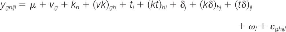the terms of which are defined in Table II. The random-effect terms were specified to account for the sources of variance listed in Table I although we emphasize that the model terms generally accounted for aggregate effects of the specific sources of variance (i.e. they are “lumped” parameters). For example, ω_l, the between-well or between-sample main effect, represented the sum of effects of all the factors listed in the “Between well or sample” column of Table I. However, some terms did account for distinct technical factors, such as the (tδ)_ij term, which accounted for the day-specific differences in the concentrations and/or specific activities of the ligands (Table II, “Between Day” column). We note the special case of k_h (the “Kit” or analyte main effect), which accounted for both biological and technical factors; specifically, k_h represented the effects of the analytes as well as their corresponding assay kits, with the analyte effects presumably caused by their different total protein abundances and the assay kit effects presumably caused by differences in antibody properties such as binding affinities.

Table II. Specification of the full model.

Algebraic model terma	Variable or factor	Effect type and assumptionb	Subscript range (main effects) or number of terms (interactions)	Terms in the computational modelc
yghijl	Response variable			log10(MFI)
μ	Mean MFI of phospho-Akt measurements from vehicle-treated samples		1	Intercept
vg	Vehicle main effects	Fixed	g = 1,2	(ligand vehicle)d, dmso
kh	Kit (analyte) main effect	Fixed	h = 1–16	(akt)d, erk, gsk, ikb, jnk, p38, p70, p90, cjun, creb, hsp27, irs, mek, p53, stat3, s6rp
(vk)gh	Vehicle × Kit interaction	Fixed	15	dmso × 15 kits
ti	Treatment main and interaction effects	Fixed	i = 1–17	Main: d, 6, L, N, G
				2-way interactions: d×6, d×L, d×N, d×G, 6×L, 6×N, 6×G, N×G
				3-way interactions: d×6×L, d×6×N, d×6×G, d×N×G
(kt)hi	Treatment × Kit interactions	Fixed	17 treatment effects × 15 kits = 255	Each treatment term × 15 kits
δj	Day main effect	Random	j = 1–3	d1, d2, d3
		d∼N(0,σd2)
(kδ)hj	Day × Kit interaction	Random	3 days × 16 kits = 48	Each day term × each of the 16 Kit terms
		(kd)∼N(0,σkd2)
(tδ)ij	Day × Treatments (main effects only) interaction	Random	3 days × 5 treatments × 2 levels of each treatment = 30	Each day term × each of d, 6, L, N and G
		(td)∼N(0,σtd2)
ωl	Well (sample) effects	Random	l = 1–86	Well addresses (e.g., A9, G12, etc.)
		w∼N(0,σw2)
ϵghijl	Residual error	Random
		e∼N(0,σ2)

^a The algebraic equation is a compact representation of the mixed-effects model that must be translated into a computationally readable form. Although R can handle categorical variables specified in compact form (e.g., specifying a factor such as “Kit” and listing its constituents as levels in the data column), doing so precludes eliminating terms from within that factor during variable selection. We therefore explicitly specified each level of the factor as its own term in models subjected to variable selection. See the spreadsheet file in the Supplementary Information for more details.

^b The random effects were assumed to be independent values of their respective variables that are normally distributed with mean of zero and variance as indicated.

^c Legend: d = Dexamethasone, 6 = interleukin-6, L = interleukin-1α, n = tumor necrosis factor-α, G = transforming growth factor-α, d1 = Day 1, d2 = Day 2, d3 = Day 3.

^d Terms listed in brackets did not have their own terms in the computational model but instead served to estimate the intercept, relative to which the effects of the remaining terms were computed.

We note that the model above incorporates all known sources of variance and is therefore a single “global” model. Our global approach might be counterintuitive because usually one thinks of the signals (analytes) as independent response variables. Furthermore, precedence exists for fitting separate models to each gene in the analysis of microarray and genetic screen data in order to facilitate computationally tractable analysis (e.g. 18, 23). Indeed, univariate statistical methods are commonly used for analyzing multiplexed bead-based data (10, 13, 16), which is akin to fitting separate models for each phospho-protein analyte. Doing so, however, sacrifices the numerous benefits of the global approach. First, a principal advantage of specifying a global model is that the effects are estimated in context of one another, which can strengthen the validity of the associated inferences (9). Second, the global modeling approach provides the most degrees of freedom for estimating effects, especially once nonsignificant terms are eliminated through variable selection. In addition, the global modeling approach accounts for the degrees of freedom allocated for normalization (17). Therefore, we implemented the global approach by defining the response variable as the log-transformed MFI values from the Bio-Plex instrument and we classified each phospho-protein analyte as a predictor variable, represented by the k_h term in the algebraic model. We evaluated whether a treatment significantly affected the levels of an analyte by examining the corresponding treatment-by-kit interaction term.

Once the model terms were determined, we classified each term as fixed or random (Table II, Supplementary Information). The distinction between fixed and random effects lies in the inferences to be made. Terms are assigned as fixed if they represent factors whose levels featured in the experiment are of specific interest and the inferences about those factors are restricted to those levels (25, 26). Random-effect terms are used to represent factors whose levels are considered to be randomly sampled from a population of theoretically infinite size and the inferences about that factor apply to the population of its levels (25, 26). In practice, terms for continuous factors, i.e. those whose levels can assume any value such as ligand doses, are almost always set as fixed effects (25). Also, factors corresponding to experimental treatments are usually specified as fixed-effect terms whereas nuisance factors are usually considered as random-effect terms (25). We followed these guidelines in specifying the terms in our model: Terms associated with biological (treatment) factors were considered fixed, whereas technical factors (Day and Well) were assigned as random effects (Table II). There was one special case: Terms associated with DMSO treatments, which we considered a technical factor, were assigned as fixed effects because the concentration of DMSO is a continuous variable. In the case of an interaction term containing both fixed and random effect terms, the interaction term must be random (25); thus, interaction terms involving the factor “Day” were random.

The algebraic model was translated into a computational model, with each term described in Table II. The model was implemented using the “lme4” package (version 0.999375–42) in the software R (version 2.14.0), which employs the restricted maximum likelihood criterion to optimize the effect estimates. We also fitted the model using the maximum likelihood criterion in order to compute the Akaike Information Criterion and the Bayesian Information Criterion (28). Plots and additional analyses were performed in Excel (Microsoft) and Matlab (The MathWorks). In general, mixed-effects models provide different types of estimates for the fixed and random effects. For fixed-effect terms, the model estimates the effects with their uncertainties as model coefficients with standard errors, respectively. For the random effects, the model estimates the variance of the population from which the levels of the random-effect terms were drawn. Therefore, an additional advantage of specifying a term as a random effect is that only a single parameter is estimated for that term no matter how many levels the corresponding factor includes. We still obtained effect “estimates” for the levels of a random factor, known as the best linear unbiased predictors (BLUPs) (25, 26), and we used these to normalize the data. Further details on the distinction between estimating fixed-effects parameters and the random effects are provided elsewhere (28).

Variable Selection and Data Normalization

In conducting the statistical modeling, we sought the simplest model that fit the data well. We started with the fully specified global model (the “full” model) and simplified it by removing terms through variable selection. The performance of the resulting models was assessed using several metrics including the Akaike Information Criterion (AIC), the Bayesian Information Criterion (BIC), the Pearson correlation between the fitted values and the observed data (r_fit), model predictivity as assessed by the Pearson correlation between the observed and predicted values from leave-one-out cross-validation (r_LOOCV), Gaussian distribution of the residuals as assessed by the Shapiro-Wilk test (P_SW) and a signal-to-noise ratio (SNR) defined as the ratio of standard deviations of the model fits to the residuals (21). We eliminated terms from the model if their 95% highest probability density (HPD) intervals encompassed zero, unless their inclusion was merited by hierarchy principle considerations (i.e. lower-level terms that are the basis for significant higher-order interaction terms should be retained in the model even if they themselves were not statistically significant (7)). The HPD intervals were calculated via Markov Chain Monte Carlo (MCMC) sampling implemented in the “pvals.fnc” function in the “languageR” package (version 1.2). Variable selection was iteratively performed as above until all the terms were significant, at which point outliers were removed. Observations were assigned as outliers and eliminated if their residuals caused the distribution of residuals to clearly depart from Gaussian (7, 26). After outlier removal, a final round of variable selection was performed to obtain the final model.

Once the final model was obtained, we normalized the data by subtracting the technical effects from each observation in the data set according to the following equation:

Note that the DMSO effect was subtracted from observations featuring either DMSO or dexamethasone treatments, because DMSO was the vehicle for dexamethasone.

We compared the final model to a regression model that incorporated only the fixed effects terms from the mixed-effects model. The regression model was computed using the ‘lm’ function in R.

Constrained Fuzzy Logic Modeling

We modeled two data sets using constrained fuzzy logic (cFL): The raw data and the normalized back-transformed data in which the data was log-transformed, normalized and then taken to the power of ten to reverse the log transformation. We scaled the MFI values from both the raw data and the normalized back-transformed data for each analyte under each condition between zero and one by dividing the relative-fold increase of the signal value in the stimulated versus unstimulated condition by the maximum relative-fold increase observed for that analyte across all conditions. A cFL model was trained to both data sets (raw and normalized back-transformed) using previously described methods (29). Briefly, a prior knowledge network (PKN) was constructed from literature-curated molecular pathways and interactions known to exist between the ligands used in the experiments and the measured analytes. After structural processing of the PKN to compress nodes that were neither measured nor perturbed, the network was converted into a cFL model. The topology and parameters of this model were trained simultaneously using a genetic algorithm that, for each interaction, chooses one of a predefined set of mathematical functions to relate the input and output species, including the possibility that they do not relate. Finally, a heuristic reduction and refinement step was carried out to remove interactions that were not necessary to fit the data. The resulting trained models contained only interactions that were consistent with the data and were thus used as a tool to determine if the data was consistent with the PKN.

Data Presentation and Statistical Significance Testing

The boxplots presented in this paper were defined as follows: A red horizontal line represented the median and the horizontal edges of the boxplots represented the 25th and 75th quartiles such that the box spanned the interquartile range. The whiskers extend 1.5× the interquartile range from the boxplot edges, while values outside of the whiskers were denoted as red “+” symbols.

Several methods were used to test for statistical significance. For the mixed-effects and regression models, we tested the null hypothesis that each term's effect was equal to zero. In the case of the mixed-effects models, the HPD interval software described above provided both an empirically derived p-value estimate as well as a t test-based estimate for each term. For the regression model, the test of statistical significance was a t-test (7). In addition, we tested whether the deviation of the Well effect means for each row and column were statistically different from zero using an empirical test. Specifically, we randomly shuffled the Well effects relative to their actual well addresses and recomputed the row- and column-specific means 10,000 times. We then estimated the probabilities of the observed means by determining their locations within the 10,000 resampled means. For all tests, the level of significance was set at 0.05 and adjusted for multiple comparisons by controlling the false discovery rate (30).

RESULTS

Hepatocyte Inflammatory Signaling Experiment

We studied hepatocyte intracellular signal transduction leading to acute-phase protein secretion. We modeled this scenario in vitro using HepG2 cells exposed to combinations of the inflammatory cytokines IL-6, IL-1α, and TNF-α, in addition to the stress-responsive glucocorticoid hormone analog dexamethasone and the growth factor TGF-α (Fig. 1A). We measured the levels of 16 phospho-proteins that operate as part of receptor-mediated signaling pathways downstream of the applied ligands using Bio-Plex multiplexed bead-based immunoassays (Fig. 1A). The design featured combinatorial treatments of dexamethasone, IL-6, TNF-α, and TGF-α, as well as IL-1α applied combinatorially with dexamethasone and IL-6 (Fig. 1B, Supplementary Spreadsheet file, “Arrayed data” worksheet). Ligand vehicle and DMSO controls were also included (Figs. 1B and 1C). One replicate of each condition was performed on each of three different days with the exceptions of the vehicle control, DMSO control, and the dexamethasone conditions, which were applied twice as within-day biological replicates on each day (Fig. 1C). For the Bio-Plex assay, we also performed technical replicates. One of the between-day biological replicates from each condition was randomly chosen to be applied twice to the assay plate (Figs. 1B and 1C). Hence, each condition had a total of at least four replicates: Three between-day replicates and one technical replicate. The DMSO and vehicle conditions featured seven total replicates: Two within-day biological replicates collected on each of the 3 days and one technical replicate. The dexamethasone condition had eight total replicates: Two within-day biological replicates collected on each of the 3 days and two technical replicates. We therefore assayed a total of 86 samples. To round out the Bio-Plex assay 96-well plate, we added duplicates of positive and negative control lysates for each analyte supplied by the manufacturer. Each of these controls behaved as expected (data not shown) and they were not included in the mixed-effects model analysis.

Fig. 1.

Experimental design and raw data. A, A schematic view of the experiment. We investigated the cell signaling network of HepG2 cells by treating the cells with combinations of the ligands (green) including the inflammatory cytokines interleukin-6 (IL-6), tumor necrosis factor-α (TNF-α), interleukin-1α (IL-1α), the glucocorticoid hormone analog dexamethasone (Dex) and the growth factor transforming growth factor-α (TGF-α). We used multiplexed bead-based immunoassays to measure the levels of phospho-proteins (blue) that function in intracellular signaling. The full names of the phospho-proteins are listed in the Materials and Methods section. B, Design matrix and raw data. The design matrix (at left) is shown with the columns pertaining to the replicate types, defined in panel C, shaded in orange. The filled boxes indicate the samples for which the corresponding treatments were applied. For the Day column, the unfilled boxes denote Day 1, the boxes filled gray denote Day 2 and the boxes filled black denote Day 3. The raw data is presented on the right as a heat map with one column for each of the 16 phospho-protein analytes and each row representing a single replicate of a particular condition. The colors represent MFI values spanning 68 to 26,103. C, Definition of replicate types. Our experiment featured three types of replicates: (1) Between-day biological replicates (“Day”), which we defined as cells independently treated with the same experimental perturbation but on different days (batches), (2) Within-day biological replicates (“Biol”), which we defined as cells independently treated with the same experimental perturbation on the same day (i.e. in the same batch), and (3) Technical replicates (“Tech”), which we defined as biological samples that were divided and pipetted into separate wells in the Bio-Plex assay plate. These replicate types are subject to different types of variance: Technical replicates are subject to variance introduced in the assay process, within-day biological replicates are subject to both assay variance and variance introduced by the act of experimentally manipulating the cells and between-day biological replicates are subject to the previous sources of variance in addition to batch effects.

Model Building and Performance

Preliminary analysis of the raw data indicated that it exhibited considerable variability. In general, each analyte presented a typical range of signal (MFI) as indicated by the heterogeneity of color between columns in the heat map in Fig. 1B. In all cases, the principal putative downstream signals of the ligands applied in the experiment showed increased phosphorylation after 30 min. For example, TGF-α treatment markedly increased phospho-Akt levels, while IL-1α treatment increased phospho-IκB-α and phospho-JNK levels (Fig. 1B). However, reliably identifying treatment effects was difficult by visual inspection alone. Furthermore, additional preliminary plots of the raw data showed that the Day factor contributed substantial variance. These analyses revealed that the data could benefit from normalization to remove unwanted technical variance and from statistical analysis to detect subtle but significant effects. We proceeded to accomplish these tasks using mixed-effects modeling.

We constructed a “full model” that contained terms representing all the sources of variance for which we could account. The full model contained 304 fixed-effects terms and 8 random-effect terms with a total of 167 levels (Table II; Supplementary spreadsheet file, “Full model” worksheet). We then evaluated the performance of the full model using the metrics listed in the Materials and Methods (Table III, Figs. 2A–2D). We found that the full model performed well, as indicated by the very strong correlation (r = 0.99) observed between the model fit and data (Table III, Fig. 2A). However, the effect estimates for many terms were not statistically significant (Supplementary spreadsheet file, “Full model” worksheet), which suggested that they could be eliminated without detrimentally affecting model performance. Indeed, eliminating these terms markedly lowered the BIC but only marginally affected the goodness-of-fit (Table III). In the second-to-last step of the variable selection, we eliminated six outliers on the basis that these values caused the residuals to depart from Gaussian distribution, as shown by the points deviating from the red dashed line at each end of the curve in the normal probability plot (Fig. 2D, red arrows). Four outliers were measurements involving phospho-IκB-α, three of which were from DMSO-treated samples and the other from a TGF-α-treated sample. The other two outliers were measurements of phospho-STAT3 in response to IL-6 and IL-6 plus TNF-α. Interestingly, measurements of phospho-IκB-α and phospho-STAT3 represented 13 of the top 15 residuals with respect to magnitude. Upon removal of the outliers, the distribution of the residuals approached Gaussian, as indicated by the closer alignment of the data to the red dashed line in the normal probability plot (Fig. 2H) and an increase in the p-value in the Shapiro-Wilk test (Table III).

Table III. Variable selection metrics.

Modela	Modifications	Selection criteria
		AICb	BICb	rfit	rLOOCV	SNR	PSW
1	Full model	−2653	−1016	0.992	0.989	9.2	<3 × 10−16
2	Remove terms	−2741	−1827	0.994	0.988	8.5	<3 × 10−16
3	Remove terms	−2772	−1988	0.993	0.990	8.5	<3 × 10−16
4	Remove terms	−2772	−2113	0.993	0.990	8.3	<3 × 10−16
5	Remove terms	−2807	−2426	0.993	0.990	8.1	<3 × 10−16
6	Remove terms	−2806	−2446	0.992	0.990	8.1	<3 × 10−16
7	Remove outliers	−2981	−2621	0.993	0.992	8.7	2.1 × 10−6
8	Remove terms (“Final model”)	−2983	−2628	0.993	0.992	8.7	2.1 × 10−6

^a Eight iterations of variable selection were performed, each resulting in a different model.

^b The AIC and BIC metrics were computed from models fit according to the maximum likelihood criterion instead of the restricted maximum likelihood criterion because the former is required for correct AIC and BIC estimates (28).

Fig. 2.

Model fits and residual analyses. A and E. Scatterplots of the fitted values from the models (“Model fits”; full model, A, and final model, E) and the observed data (“Data”). The diagonal line represents the line of unity. Note the close correspondence of the model fits to the observed data, suggesting that the model fit the data well. B and F. Scatterplots of the residuals and the model fits. The residuals were distributed evenly around zero and exhibited no functional dependence on the magnitude of the fitted values, thus supporting the assumptions of homogeneous variance and independence (full model, B, and final model, F). C, D, G, and H. Histograms (C and G) and normal probability plots (D and H) of the residuals were plotted for the full (C and D) and final (G and H) models. The presence of outliers (identified in D by the red arrows) in the data set used to fit the full model caused the residuals to deviate from Gaussian distribution. Eliminating these outliers and fitting the remaining data to the final model led to residuals that were approximately normally distributed (compare panels D and H).

The final model featured 62 fixed-effect terms and five random-effect terms containing 149 levels (Supplementary spreadsheet file, “Full model” worksheets), yet performed almost equivalently to the full model with respect to goodness-of-fit (Fig. 2E) and predictivity (Table III, r_LOOCV) and better with respect to parsimony and residual behavior (Table III, Fig. 2D versus 2H). The residuals for both the full and final models were homogeneously distributed as a function of the model fits (Figs. 2B and 2F), which validated our assumption of variance homogeneity for the log-transformed MFI data. The random effects were also approximately normally distributed (Supplemental Fig. S1).

Normalization Increases the Observed Precision and Sensitivity of the Multiplexed Bead-based Immunoassay Data and the Accuracy of Downstream Biological Analysis

With the final model in hand, we normalized the data by subtracting the effect estimates of the technical factors from the observed data (Supplementary Spreadsheet file, “sm8 analysis” worksheet). The normalized data was clearly less variable, due chiefly to the removal of the Kit main effects and terms involving Day (Fig. 3). Next, we used the model effect estimates to investigate the ligand effects on each analyte (Fig. 4; Supplementary Spreadsheet file, “sm8 analysis” worksheet). We observed that IL-1α and TGF-α treatments markedly increased the levels of most phospho-proteins whereas IL-6 and TNF-α treatments increased the levels of only a few phospho-proteins (STAT3 for IL-6 and IκB-α, JNK, and c-Jun for TNF-α) (Fig. 4); the capability of modeling-based normalization to discern truly significant activations can be appreciated by comparison to Fig. 1B. Such subtle treatment effects were not apparent for dexamethasone (Fig. 4), which suggested that the effects observed for the other ligands were real. In addition, we plotted the same data except with the Day and Well effects added. We observed that the Day and Well effects contributed considerable variability as indicated by the elongated boxplots (Fig. 4, right panels). The additional variability blurred the distinction of phospho-protein levels from the untreated versus treated conditions seen with the normalized data.

Fig. 3.

Normalization of the data using the final mixed-effects model. A, Heat maps showing the raw, log-transformed and normalized data. Two heat maps for the normalized data are shown, the one above in which the colorbar was scaled to the entire matrix of values (“Scaled to matrix”) and the one below in which the colors were scaled to the values within each column (“Scaled to column”) to more clearly represent the treatment effects. The colorbars correspond to the MFI or log MFI values except that of the “Scaled to column” heat map, which represents log MFI values rescaled to 0 to 100. B, Boxplots of the log-transformed and normalized data grouped by analyte and by day (the three boxplots for each analyte represent in order the data from days 1, 2, and 3). Note that the boxplots of the normalized data are aligned at a log MFI of just under 4. The scaling of the data to this particular value was because of all the effects being computed relative to phospho-Akt (for the sole reason that it was alphabetically the first term among the Kit effects) such that the data was normalized relative to its average log MFI in the vehicle-treated condition (log MFI = 3.85, corresponding to MFI ∼ = 7,100). The details of the boxplot construction are presented in the Materials and Methods section. RFU = relative fluorescence units.

Fig. 4.

Ligand main effects on phospho-protein levels with and without technical variance. Boxplots of the normalized log MFI for each analyte were plotted as a function of the presence (turquoise) or absence (red) of each ligand shown at the far right. For the panels on the left, the plotted values were computed by summing the mixed-effects model estimates of the intercept, the residuals and the effects for the all the terms that included the ligand specific to that panel, thus representing normalized data. The panels on the right feature those same values except with the Day and Well effects added, thus representing nonnormalized data. The variability contributed by the Day and Well factors is indicated by the elongated boxplots in the right panels versus those in the left panels. The details of the boxplot construction are presented in the Materials and Methods section. RFU = relative fluorescence units.

By eliminating systematic variance in the data, normalization should benefit its downstream analysis. We evaluated our expectation with three analyses. First, we found that the coefficients of variation (CV) calculated from the replicates of each experimental condition (Supplementary Spreadsheet file, “sm8 analysis” worksheet) were generally reduced for the normalized data, as indicated by the data points located mostly below the line of unity (Fig. 5A). Specifically, 62% of the CV's calculated from the normalized data were lower than those calculated from the log-transformed data, with a maximum CV of 8% as compared with a maximum of 15%, respectively (Fig. 5A). Second, we estimated the Pearson correlation coefficients between all pairs of distinct signals (e.g. phospho-Akt versus phospho-ERK, etc.) using both the log-transformed and normalized data. We found stronger correlation coefficients and lower p-values for the normalized data as indicated by the concentration of points above and below the line of unity in each plot, respectively (Fig. 5B).

Fig. 5.

The effect of normalization on the precision and sensitivity of multiplexed bead-based immunoassays. A, Scatterplot of the coefficients of variation (CVs) of replicate data for both log-transformed and normalized data. Each data point represents a CV calculated from the replicates of a particular observation, with n = 4, 7, or 8 depending on the condition (see text for details). B, Scatterplots of the Pearson correlation coefficients (left) and corresponding p-values (right) for each pair of analytes from the log-transformed (left) and normalized data (right; n = 16² = 256 points per plot). C, Illustration of the effect of data normalization on testing for statistical significance. The upper and lower panels feature boxplots from the log-transformed and normalized data, respectively, that show the effect of TNF-α and TGF-α factorial treatments on MFIs for Akt, JNK and p38 MAPK. Akt is shown because it is the basis for comparison in the mixed-effects model. n = the number of observations contributing to the corresponding boxplot above. The boxplots for the normalized data are generally shorter than those for the log-transformed data and thus indicate reduced variability. The details of the boxplot construction are presented in the Materials and Methods section.

Third, we evaluated the sensitivity of the mixed-effects model for discriminating statistically significant terms. Specifically, we compared the mixed-effects model to a regression model that contained the same fixed-effects terms as the final model but that lacked the random-effect terms associated with the Day and Well factors. Removing the random-effect terms shifted the variance of those terms into the residual variance of the regression model. The residual variance in part determines the standard errors of the effect estimates. If the residual variance is higher, then the standard errors will be as well, with the consequence of reducing the probability of detecting differences between means. Accordingly, we observed that several terms were statistically significant in the mixed-effects model but not in the regression model (Supplementary spreadsheet file, “Compare models” worksheet). Two examples were the three-way interaction terms of TNF-α ×TGF-α × phospho-JNK and TNF-α × TGF-α × phospho-p38 MAPK (Table IV), which indicated non-additive effects of TNF-α and TGF-α on these analytes. We observed that the effect estimates were similar but that the standard errors for these estimates were almost double for the regression model (Table IV, Supplementary spreadsheet file, “Compare models” worksheet), which reflected the higher variability observed in the merely log-transformed data compared with the normalized data (compare boxplot lengths in the top versus bottom panels of Fig. 5C).

Table IV. Mixed-effects model estimates and statistics for three-way interactions involving TNF-α and TGF-α treatments.

Model terms	Modela	Coefficient	Standard Error	t-value	p-valueb
N × G × JNK	1	0.098	0.032	3.10	0.002
	2	0.087	0.062	1.42	0.157
N × G × p38	1	0.125	0.028	4.41	<0.001
	2	0.096	0.055	1.75	0.081

^a Model 1 was the final mixed-effects model and Model 2 was a regression model equivalent to Model 1 except that it lacked the random-effect terms. Model 2 was fit using the “lm” function in R.

^b The p-values for the two models were computed using different techniques, such that they are only roughly comparable. The p-values for the terms in Model 1 were both significant at the 0.05 level after correcting for multiple comparisons using the false discovery rate, whereas the p-values for Model 2 did not achieve significance.

Finally, we evaluated the effect of data normalization on the interpretations gleaned from a network-level modeling technique, constrained fuzzy logic (cFL), which seeks to deduce multipathway influences among protein signals (29). We applied cFL modeling to explore the hepatocyte signaling network underlying the secretion of acute-phase proteins. The principal ligands involved in acut-phase protein secretion are IL-6, IL-1α, and glucocorticoid hormones (of which dexamethasone is a synthetic analog), which prompt the secretion of proteins such as fibrinogen, serum amyloid A and haptoglobin (Supplemental Fig. S2). Although IL-6 and IL-1α function through well characterized signaling pathways, the mechanisms by which other modulatory ligands act are less clear.

Glucocorticoid hormones directly regulate transcription by translocating into the cell, binding steroid receptors and then binding DNA (31). However, glucocorticoid hormones may also regulate signaling events via membrane-bound glucocorticoid receptors (15, 32). Therefore, we evaluated the possibility that dexamethasone influenced the levels of the phospho-proteins in our system. To test this notion, we trained cFL models using a prior knowledge network in which we introduced edges connecting a node representing dexamethasone to nodes representing the measured phospho-proteins (Supplemental Fig. S3A). We note that a family of models, which are essentially equivalent with respect to goodness-of-fit, is typically produced (29). If the edges were consistent with the data, then the cFL algorithm would retain the edges in the resulting family of fitted models. This approach assumed that the data faithfully reflected the biology—if it did not then the approach would become vulnerable to false positives or false negatives. By extracting technical sources of variance, normalizing the data helps to ensure that the data is at least predominantly a function of the biological sources of variance. To evaluate the effect of technical variance in data used for cFL modeling, we compared cFL models trained using either the raw or normalized back-transformed data. When the cFL models were fit to the raw data (Supplemental Fig. S3B), we observed edges between dexamethasone and the phospho-proteins in many of the models, which was indicated by the thicknesses of the edges (Fig. 6). In the case of cFL models fit to the normalized back-transformed data (Supplemental Fig. S3C), few of the models contained edges between dexamethasone and the signals, indicated by the faint lines between dexamethasone and four of the downstream signals (Fig. 6). Qualitatively distinct results of the cFL modeling were therefore obtained according to whether the models were fit to the raw or normalized back-transformed data, indicating the significant impact that technical variance in the data can have on cFL modeling.

Fig. 6.

Constrained fuzzy logic models trained to raw and normalized data. The cFL model algorithm takes as input a prior knowledge network and experimental data and retains the edges are required to best fit the data. The green nodes represent the ligands applied in the experiment, the blue nodes represent measured phospho-proteins and the white nodes represent molecules that were neither measured nor perturbed but whose retention in the model was necessary for logical consistency. The thickness of an edge is proportional to the number of models within the family of trained models in which the edge was retained and thus reflects the likelihood that the connection the edge represents exists in reality. CFL models trained to the raw data indicated that several edges between dexamethasone and phospho-proteins were consistent with the data. In contrast, cFL models trained to the normalized back-transformed data contained only edges of very low confidence between dexamethasone and four of the phospho-proteins.

Analysis of the Technical Sources of Variance

The mixed-effects model algorithm provides “estimates” of the random effects in the form of BLUPs (26, 28). These estimates provide a means to analyze how the data were affected by the technical factors, which could lead to important insights into quality control and experimental design strategies for multiplexed bead-based immunoassay experiments. We first compared the effects of the technical factors relative to each other and to the biological effects. To do so, we calculated the percentage variance of the technical and biological factors on each observation using the following formula:

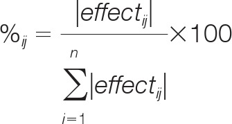where %_ij is the percent variance contributed by the i^th effect to the total variance of observation j. We then summed the percent variances associated with the biological factors for each observation and plotted them against the percent variances contributed by each technical factor (Fig. 7, Supplementary Spreadsheet file, “Var_contrib” worksheet). In general, the biological factors contributed most of the variance to each observation, indicated by the grouping of the data in the lower right quadrants of the plots (Fig. 7). However, the plots reveal a number of cases in which the technical factors contributed as much or more variance than the biological factors, as indicated by data points in the center and upper left quadrants of the plots (Fig. 7). In general, we observed that the Day factor contributed proportionally the highest amount of variance among the three technical factors because the distribution of points in the Day plot was shifted upward compared with those in the Well and DMSO plots (Fig. 7).

Fig. 7.

The contributions of the biological and technical factors to the total explained variance. Scatterplots show the percent contributions to the total explained variance by the biological (treatment) and the individual technical factors (Day, Well, and DMSO) for each measurement (n = 1376). Each plot features a scatter of points triangular in shape, which is expected because the sum of the percent variance contributions cannot exceed 100%. A data point in the lower right quadrant of a plot means that the biological factors contributed more variance than the indicated technical factor for that observation whereas the converse was true for a data point in the upper left quadrant.

Next, we searched for additional technical factors that may have affected the assay but for which we did not account in the model. In particular, we were concerned about order and position effects in the assay plate. Order effects arise if the sequence in which the samples were loaded onto the assay plate contributed systematic variance. Position effects refer to the row and column effects that are sometimes observed in plate-based assays (33). Because we randomly assigned samples to wells on the assay plate, any order or position effects, if present, should manifest themselves as patterns in either the Well effects or the residuals. In accordance with the randomization of sample assignments to the wells, we observed no obvious patterns in the assignment of samples to the assay plate (Fig. 8A). We then plotted the Well effects and residuals as a function of loading order and plate row and column and searched for patterns and substantial deviations from zero. Both the Well effects and residuals were independent of loading order (Fig. 8B) and the residuals were independent of the plate rows and column (Figs. 8C and 8D, right panels). Some variation was observed among the Well effects as a function of the rows and columns but these deviations were not statistically significant (p > 0.05 after correction for the false discovery rate; Figs. 8C and 8D, left panels). The Well effects' variation with position relative to the residuals is reasonable because the sample sizes associated with the Well effects were considerably smaller than for the residuals (n = 9–12 for rows and n = 6–8 for columns for the Well effects versus n = 144–192 for rows and n = 96–128 for columns for the residuals). We concluded that our data were free of order- and position-related technical effects.

Fig. 8.

Evaluation of order and position as possible technical factors. A, Plots of the randomized assignment of samples to the wells of the Bio-Plex assay plate. A filled well denotes that its corresponding sample was treated with the ligand labeled above the plate. A well filled for multiple ligands simply denotes a sample that was treated with a combination of ligands. Note the absence of obvious patterns in the assignment of samples to the assay plate. B, The well effects (left) and residuals (right) were plotted as a function of sample loading order in the Bio-Plex assay plate. The samples were loaded in vertical order, i.e. from well A1 to H1, A2 to H2 and so forth until well H12. A single well effect and 16 residuals were associated with each well, such that we used a bar chart to visualize the Well effects and boxplots to visualize the residuals. The details of the boxplot construction are presented in the Materials and Methods section. Note the lack of obvious patterns in the Well effects plot and the centering of the boxplots at zero in the residuals plot. C and D, Well effects (left) and residuals (right) were plotted as a function of plate column (C) and plate row (D) in the Bio-Plex assay plate. Scatterplots and boxplots were used to visualize the Well effects and residuals, respectively, because the Well effects featured only a few data points (n = 6–12) per group compared with the residuals (n = 96–192; see main text for more details). Position effects would be indicated by an obvious deviation of the average of the data points or boxplots from zero, which we did not observe here.

DISCUSSION

We report here the use of mixed-effects modeling to normalize and statistically analyze multiplexed bead-based immunoassay data. Specifically, we fit a single global model to the data that included terms representing each of the biological and technical factors for which we could account. The model provided estimates of the effects associated with these factors. We then normalized the data by subtracting the technical effects, which left as remainder the intercept, the biological effects and the residual error. We used this normalized data for further analyses.

Benefits of Processing Bead-Based Assay Data Using Mixed-Effects Models

We found that the mixed-effects model offered exceptional insight to our data. By deconvoluting the biological and technical effects, we could analyze them in isolation. Removing the technical effects via normalization led to inferences about the biological effects that were of higher confidence owing to improved precision and sensitivity (Figs. 4 and 5, Table IV). This was particularly true for interaction effects such as those between TNF-α and TGF-α in promoting JNK and p38 MAPK phosphorylation. The significant interaction term indicated a synergistic effect of TNF-α and TGF-α on the phospho-levels of these proteins. Functionally important synergy between these two ligands has been previously found in human mesenchymal stem cells for secretion of hepatocyte growth factor (HGF) and vascular endothelial growth factor (34, 35). In the case of HGF secretion, the synergy was dependent on p38 MAPK signaling (34). Analogous synergy between TNF-α and TGF-α in our hepatic systems is likely physiologically important because signaling from their respective downstream receptors, the TNF receptor and epidermal growth factor receptor, regulates acute-phase protein secretion (27, 36). Synergistic and antagonistic relationships have been typically evaluated using methods incorporating Bliss independence or Loewe additivity, which are widely featured in drug combination studies (37). Applying these methods to evaluate synergy between TNF-α and TGF-α would require a separate set of dose-response experiments and our results motivate further investigation in this regard.

We note that the data featured in this study were generated from experiments in which saturating doses of ligands were used, which elicited biological effects of maximal magnitude. Even with these maximal effects, the technical effects still contributed proportionally substantial variance in many cases (Fig. 7), such that the analysis benefitted from normalization. We expect that the analysis of experiments with treatments featuring submaximal doses of ligands or small-molecule inhibitors, such as dose-response experiments, would especially benefit from normalization using mixed-effects models because the biological and technical effects would be expected to exhibit lesser and similar magnitudes, respectively, to those observed in the experiment reported in this paper.

Normalizing the data with mixed-effects models can benefit downstream analysis of the data using mechanistically oriented network-level modeling methods such as those based on differential equations or logic models (38, 39) or data-driven statistical frameworks (e.g. principal components analysis, partial least squares regression, clustering, etc.) (40). Such models are used to integrate the data from large multivariate data sets to infer network topologies, to quantify the strength of connections between network nodes and to predict the effects of perturbations (2, 38, 40, 41). The biological relevance of the model predictions is intimately linked to the degree to which the data is a function of the biology, which can be compromised by the presence of technical effects. Here we observed that cFL models fit to raw and normalized back-transformed data gave qualitatively different outputs in which fewer edges between dexamethasone and measured signaling nodes were observed in the models from the normalized data (Fig. 6). These results have opposing biological interpretations: Model outputs based on the raw data implied that dexamethasone somehow promoted the phosphorylation of certain signaling proteins whereas outputs based on the normalized back-transformed data implied that dexamethasone did not regulate signaling.

We cannot definitively conclude that more physiologically correct cFL models resulted from using the normalized data, but they do match our expectations from known biology and our data. Specifically, despite the existence of evidence for glucocorticoid hormones being able to regulate cell signaling (15, 32), their principal mode of action is direct transcriptional regulation (31), such that we expected dexamethasone to have little to no effect on phospho-protein levels. Accordingly, we observed that dexamethasone treatment for 4 hours did not alter phospho-protein levels (Fig. 4). The apparent discrepancy between the data (Fig. 4) and the cFL models (Fig. 6) with respect to dexamethasone arose because the cFL algorithm is sensitive to the increase in signal on stimulation compared with its vehicle control, which in this case involved the signals in response to dexamethasone and DMSO being compared (Supplemental Fig. S3B, dex = 1 column). Variance induced by the technical factors caused slight increases in some signals in the dexamethasone-treated samples compared with DMSO (Supplemental Fig. S3B). In contrast, the plot in Fig. 4 featured all of the observations grouped according to whether they were treated with dexamethasone. The ability to rigorously normalize the data allows us to retain the sensitivity of the cFL algorithm while defending against possible false positive results caused by technical variance. We note that normalizing the data by mixed-effects modeling could precede the other types of network-level models such that it represents a general strategy for improving data quality.

Mixed-effects modeling of the data presents an additional possible benefit for network-level modeling. Mixed-effects models provide an estimate of the residual variance, which if all other sources of variance are accounted for in the model, represents an estimate of the random experimental error or noise. This residual variance estimate could be used for sensitivity analyses of the network-level model to random error. Specifically, the model could be fit to synthetic data sets generated by Monte Carlo sampling of the distribution of residuals in order to determine how experimental error propagates through the modeling algorithm and affects the predictions.

We also used the mixed-effects modeling approach to obtain insights into the properties of the technical factors. We compared the model-based estimates of the technical effects and observed that the Day factor contributed the most variance (Fig. 7). This result has two important implications: First, assay reproducibility should be evaluated with experiments performed on different days (or in different batches) and second, the experimental design and analysis should guard against potential batch effects (c.f. 6). We expand on these thoughts in the subsection below on experimental design. Furthermore, we found no evidence that additional technical factors such as order or position were present in our experiments. This result instills further confidence in the robustness of multiplexed bead-based immunoassays.

We used the totality of the data for classifying measurements as outliers. By definition, an outlier is an observation whose value lies outside the typical range of values caused by the known sources of variance. By analyzing the complete data set using a model that included all the sources of variance, we quantitatively established this typical range, which is less than what might be estimated by inspecting replicate measurements or boxplots in isolation. For example, a number of red “+” markers are featured in the boxplots of Fig. 4, which represent data points that lie beyond the whiskers of the boxplot and are conventionally considered “outliers.” Here we eliminated observations whose residuals caused the distribution of residuals to substantially deviate from Gaussian distribution, which is an assumption that must be satisfied when using the model to make statistical inferences. Using this criterion, we removed a mere six observations out of a total of ∼1400. That so few observations were considered outliers demonstrates the internal consistency of our data. We do not know why those six observations were outlying and we acknowledge that it can be unfavorable to remove outliers from a data set unless valid reasons exist to do so. However, because each effect estimate was based on many degrees of freedom, removing the six outliers had little influence on these estimates (data not shown) but did ensure that the distribution of residuals approached Gaussian such that the statistical tests would be valid. Furthermore, we performed all analyses other than the statistical analysis with the outliers reinserted into the data set and found that the interpretations remained unchanged.

Mixed-effects models are advantageous compared with other methods of analysis. Experiments with random factors can be analyzed with analysis of variance (7). However, analysis of variance techniques for designs with random factors have important limitations, most notably that they can only accommodate balanced designs in which the same number of observations are allocated to each experimental treatment (25). Mixed-effects models offer a more flexible approach because they can handle missing data and unbalanced experimental designs (25, 42). Now that powerful software capable of fitting mixed-effects models is widely available, we expect that they will replace analysis of variance as the method of choice for analyzing biological experiments.

Implications for the Design and Conduct of Experiments

A key limitation of multiplexed bead-based immunoassays is their considerable cost. From a statistical perspective, experiments have three basic purposes: To estimate treatment effect magnitudes and their precisions and to demonstrate reproducibility. Experiments should therefore be designed to maximize efficiency in which the minimum number of observations is used to achieve these goals. In practice, this implies that the number of replicates should be minimized. A tradeoff exists, however, because replicate observations are necessary for providing the statistical power necessary to robustly estimate precision and demonstrate reproducibility. Applying a statistical model to the data allows one to minimize the replicates while maintaining statistical power (24). We discuss in detail how the use of statistical models can lead to efficient experimental designs.

Using a statistical model enables the use of three strategies for efficient experimental designs. First, statistical models enable the use of factorial designs, which involve combinatorially applying the treatment factors, rather than varying the factors one-at-a-time. Factorial designs are more efficient because they allow interaction effects to be estimated and because replication is inherently achieved due to each treatment being applied to multiple experimental units (7). Because the treatments are combinatorially applied, a statistical model is necessary to decouple the factor effects from one another. Second, statistical models can serve as the basis for estimating a priori the number of replicates necessary to achieve a desired level of precision (18, 43) such that excess replicates can be avoided.

Third, statistical models enable the use of between-day biological replicates, which allows replicates to be used to simultaneously estimate variance, contribute degrees of freedom and assess reproducibility. A key concept underlying our argument is that of statistical independence. Two events are statistically independent if the probability of occurrence of one event does not affect the probability of occurrence of the other event. In the case of observations in an experiment, statistical independence implies that the residuals of each observation are uncorrelated. A standard assumption of regression and mixed-effects models is that the residuals are independent.

Despite mathematical clarity, defining independence in practice is not straightforward. In cell biology experiments, the minimum standard for classifying replicates as statistically independent is that they be within-day biological replicates (as opposed to technical replicates; see Fig. 1C) (44). However, the threshold for independence becomes murky when certain technical sources of variance such as batch effects impinge on the experiment because they introduce systematic bias that ultimately correlates the measurements. To ensure the statistical independence of replicates, the experiment should be performed in the presence of primary threats to reproducibility such as batch effects.

A downside to replicating experiments in the presence of technical sources of variance is introducing variability that can reduce precision and decrease the probability of finding statistically significant results. Biologists therefore typically attempt to stringently control sources of variance extraneous to the experiment. In particular, experiments are usually performed using within-day biological replicates in order to avoid introducing between-day variation. Reproducibility is then assessed by conducting a separate experiment on another day and comparing the results to those from the first experiment. If the results are sufficiently similar then the experiment is considered reproducible. Typically, the data from only one of the experiments is reported in a publication (as “representative” data).

An alternative, more efficient approach depends on analyzing the data using a statistical model such as the mixed-effects model used in this study. By normalizing the variance contributed by the technical sources of variance, the use of statistical models allows the experiment to be performed using exclusively between-day biological replicates, such that replicates can be simultaneously used to estimate precision and evaluate reproducibility. The gains in efficiency with this approach can be illustrated with the following example. Suppose a biologist conducts an experiment in which three replicates of each treatment are desired. The typical strategy would involve performing one experiment with three within-day biological replicates and then repeating the experiment on a different day to ensure that the results were reproducible. Between the two experiments, six observations per treatment would be collected. The alternative approach would involve collecting a single replicate per treatment on each of 3 days to collect three between-day biological replicates. The variance introduced by performing the experiment on different days could be normalized using a statistical model containing terms adjusting for the between-day effects. The alternative approach is more efficient because it involves collecting half the number of observations per treatment (three versus six) yet features one more between-day replicate to evaluate reproducibility (three versus two). Furthermore, the data from the three between-day replicates would all be presented in a publication. Therefore, by purposefully performing between-day replicates, even if it is logistically unnecessary to do so, and using a statistical model to analyze the data, replication and reproducibility assessment can be achieved efficiently and without adversely affecting statistical power.

Caveats of Using Mixed-effects Models for Data Normalization and Analysis

The mixed-effects modeling approach has some limitations that must be considered. First, to reliably estimate the variance components of the random-effect terms, considerable replication is required. For example, the confidence intervals for the variance estimates of the Day-by-Kit interactions were large (Supplementary spreadsheet file). Therefore, if one uses the model with the intent of rigorously estimating variance components, one must ensure sufficient replication. Second, the models do not distinguish the mechanisms underlying the technical factors. For example, we know that the specific batch of an experiment contributes significant variance but the model does not tell us why; we can propose a number of reasonable mechanisms (Table I) but ultimately cannot prove their contributions. On the one hand, this feature is beneficial because known variance can still be captured without knowing its mechanisms. However it could also be possible to propose terms for the model that improve the appearance of the data but whose inclusion is not mechanistically justified. It is therefore important to justify each term in the model by considering the potential sources of variance in the experiment (e.g. Table I).

The linear mixed-effects modeling approach is powerful for the design presented here. However, other common experimental designs, such as time courses and dose-response experiments, often feature nonlinearity that must be accommodated by the model. Linear and nonlinear mixed-effects models present viable analytical frameworks for such data and several strategies are available for their implementation. First, in some cases, data transformations can sufficiently linearize the data. Second, the levels of continuous factors can be considered as distinct categorical factors, each with their own term in the linear model (21). Third, nonlinear mixed-effects models can also be used if the functional relationship between the predictor and response variables is known (45). This approach would probably be best suited to dose-response data in which sigmoidal functional relationships are commonly observed. A related approach involves using splines in a mixed-effects modeling framework, also known as semiparametric regression (46). Finally, a sequential approach could be used in which a linear mixed-effects model is used to model and normalize the technical effects, after which a modeling framework that can handle nonlinearity (such as cFL) is used to model the normalized values (which correspond to the residuals of the first model). Sequential approaches have been used in several studies to ensure computational tractability of the modeling (18, 23). Although this approach is appealing, it is important to recognize that estimates will likely be more accurate if the data is modeled using a single model (9). Our future work will seek to devise and test methods for handling nonlinear data.

We remark that the mixed-effects model approach does not require the use of housekeeping protein measurements, which often serve as a basis for data normalization. However, including housekeeping protein measurements in the experiment could improve the interpretability of the model. The model requires that a single condition be used as the basis for comparison and its value is equal to the intercept. The effect estimates for all other terms are calculated relative to the intercept, which can obscure the interpretability of those estimates. In our case, phospho-Akt was the basis for comparison such that the intercept was the average log MFI for phospho-Akt in the vehicle-treated condition. Treatment-by-Kit interaction terms distinguished the differences in log MFI values of the remaining analytes from those of Akt. So, if the log MFI of an analyte in response to a treatment was indistinguishable from that of phospho-Akt, the term in the model would be nonsignificant, even if that treatment caused a change in the levels of the analyte. Such was the case for phospho-p38 MAPK in response to TGF-α, for example (Fig. 4). If an unresponsive housekeeping protein was used as the basis for comparison instead, then the treatment-by-kit interaction effect estimates should more closely align with expectations from visually inspecting the data and therefore be more intuitively interpretable. Nevertheless, this is a minor limitation and does not adversely affect the modeling results.

In summary, we have implemented linear mixed-effects models for rigorously normalizing and analyzing multiplexed bead-based immunoassay data. Mixed-effects modeling of our data provided exceptional insights into the biological and technical factors influencing our data and improved its quality for downstream analyses. The models can serve a critical role in conducting informative and efficient experiments, thus promoting the utility and feasibility of multiplexed bead-based immunoassays. Finally, the mixed-effects modeling approach reported here is generally applicable to all types of bead-based assay data, including those used to measure cytokines, secreted proteins, intracellular proteins, and nucleic acids.

REFERENCES

- 1. Downward J. (2001) The ins and outs of signalling. Nature 411, 759–762 [DOI] [PubMed] [Google Scholar]
- 2. Clarke D. C., Lauffenburger D. A. (2012) Multi-pathway network analysis of mammalian epithelial cell responses in inflammatory environments. Biochem. Soc. Trans. 40, 133–138 [DOI] [PubMed] [Google Scholar]
- 3. Krishhan V. V., Khan I. H., Luciw P. A. (2009) Multiplexed microbead immunoassays by flow cytometry for molecular profiling: Basic concepts and proteomics applications. Crit. Rev. Biotechnol. 29, 29–43 [DOI] [PubMed] [Google Scholar]
- 4. Hsu H. Y., Joos T. O., Koga H. (2009) Multiplex microsphere-based flow cytometric platforms for protein analysis and their application in clinical proteomics - from assays to results. Electrophoresis 30, 4008–4019 [DOI] [PubMed] [Google Scholar]
- 5. Hanley B. (2007) Variance in multiplex suspension array assays: carryover of microspheres between sample wells. J. Negat. Results Biomed. 6, 6. [DOI] [PMC free article] [PubMed] [Google Scholar]
- 6. Leek J. T., Scharpf R. B., Bravo H. C., Simcha D., Langmead B., Johnson W. E., Geman D., Baggerly K., Irizarry R. A. (2010) Tackling the widespread and critical impact of batch effects in high-throughput data. Nat. Rev. Genet. 11, 733–739 [DOI] [PMC free article] [PubMed] [Google Scholar]
- 7. Montgomery D. C. (2001) Design and Analysis of Experiments, 5th Ed., John Wiley & Sons, New York, NY [Google Scholar]
- 8. Streichert T., Otto B., Lehmann U. (2011) MicroRNA profiling using fluorescence-labeled beads: data acquisition and processing. Methods Mol. Biol. 676, 253–268 [DOI] [PubMed] [Google Scholar]
- 9. Mecham B. H., Nelson P. S., Storey J. D. (2010) Supervised normalization of microarrays. Bioinformatics 26, 1308–1315 [DOI] [PMC free article] [PubMed] [Google Scholar]
- 10. Cohen G., Raupachova J., Ilic D., Werzowa J., Hörl W. H. (2011) Effect of leptin on polymorphonuclear leucocyte functions in healthy subjects and haemodialysis patients. Nephrol. Dial. Transplant. 26, 2271–2281 [DOI] [PMC free article] [PubMed] [Google Scholar]
- 11. Campbell M., Lie W. R., Zhao J., Hayes D., Mistry J., Kung H. J., Luciw P. A., Khan I. H. (2010) Multiplex analysis of Src family kinase signaling by microbead suspension arrays. Assay Drug Dev. Technol. 8, 488–496 [DOI] [PubMed] [Google Scholar]
- 12. Motazed R., Colville-Nash P., Kwan J. T., Dockrell M. E. (2008) BMP-7 and proximal tubule epithelial cells: activation of multiple signaling pathways reveals a novel anti-fibrotic mechanism. Pharm. Res. 25, 2440–2446 [DOI] [PubMed] [Google Scholar]
- 13. Bouali S., Chrétien A. S., Ramacci C., Rouyer M., Marchal S., Galenne T., Juin P., Becuwe P., Merlin J. L. (2009) P53 and PTEN expression contribute to the inhibition of EGFR downstream signaling pathway by cetuximab. Cancer Gene Ther. 16, 498–507 [DOI] [PubMed] [Google Scholar]
- 14. Jones R. J., Young O., Renshaw L., Jacobs V., Fennell M., Marshall A., Green T. P., Elvin P., Womack C., Clack G., Dixon J. M. (2009) Src inhibitors in early breast cancer: a methodology, feasibility and variability study. Breast Cancer Res. Treat. 114, 211–221 [DOI] [PubMed] [Google Scholar]
- 15. Strehl C., Gaber T., Löwenberg M., Hommes D. W., Verhaar A. P., Schellmann S., Hahne M., Fangradt M., Wagegg M., Hoff P., Scheffold A., Spies C. M., Burmester G. R., Buttgereit F. (2011) Origin and functional activity of the membrane-bound glucocorticoid receptor. Arthritis Rheum. 63, 3779–3788 [DOI] [PubMed] [Google Scholar]
- 16. Won J. H., Goldberger O., Shen-Orr S. S., Davis M. M., Olshen R. A. (2012) Significance analysis of xMap cytokine bead arrays. Proc. Natl. Acad. Sci. U.S.A. 109, 2848–2853 [DOI] [PMC free article] [PubMed] [Google Scholar]
- 17. Kerr M. K., Martin M., Churchill G. A. (2000) Analysis of variance for gene expression microarray data. J. Comput. Biol. 7, 819–837 [DOI] [PubMed] [Google Scholar]
- 18. Wolfinger R. D., Gibson G., Wolfinger E. D., Bennett L., Hamadeh H., Bushel P., Afshari C., Paules R. S. (2001) Assessing gene significance from cDNA microarray expression data via mixed models. J. Comput. Biol. 8, 625–637 [DOI] [PubMed] [Google Scholar]
- 19. Steibel J. P., Poletto R., Coussens P. M., Rosa G. J. (2009) A powerful and flexible linear mixed model framework for the analysis of relative quantification RT-PCR data. Genomics 94, 146–152 [DOI] [PubMed] [Google Scholar]
- 20. Kim R. S., Lin J. (2011) Multi-level mixed effects models for bead arrays. Bioinformatics 27, 633–640 [DOI] [PMC free article] [PubMed] [Google Scholar]
- 21. Kreutz C., Bartolome Rodriguez M. M., Maiwald T., Seidl M., Blum H. E., Mohr L., Timmer J. (2007) An error model for protein quantification. Bioinformatics 23, 2747–2753 [DOI] [PubMed] [Google Scholar]
- 22. Nahtman T., Jernberg A., Mahdavifar S., Zerweck J., Schutkowski M., Maeurer M., Reilly M. (2007) Validation of peptide epitope microarray experiments and extraction of quality data. J. Immunol. Methods 328, 1–13 [DOI] [PubMed] [Google Scholar]
- 23. Yu D., Danku J., Baxter I., Kim S., Vatamaniuk O. K., Salt D. E., Vitek O. (2011) Noise reduction in genome-wide perturbation screens using linear mixed-effect models. Bioinformatics 27, 2173–2180 [DOI] [PMC free article] [PubMed] [Google Scholar]
- 24. Ji H., Liu X. S. (2010) Analyzing 'omics data using hierarchical models. Nat. Biotechnol. 28, 337–340 [DOI] [PMC free article] [PubMed] [Google Scholar]
- 25. Galwey N. W. (2006) Introduction to Mixed Modelling: Beyond Regression and Analysis of Variance, John Wiley & Sons, Chichester, England [Google Scholar]
- 26. Pinheiro J. C., Bates D. M. (2000) Mixed-Effects Models in S and S-PLUS, Springer Verlag, New York [Google Scholar]
- 27. Baumann H., Gauldie J. (1994) The acute-phase response. Immunol. Today 15, 74–80 [DOI] [PubMed] [Google Scholar]
- 28. Bates D. M. (2010) lme4: Mixed-effects modeling with R. Springer. [Google Scholar]
- 29. Morris M. K., Saez-Rodriguez J., Clarke D. C., Sorger P. K., Lauffenburger D. A. (2011) Training signaling pathway maps to biochemical data with constrained fuzzy logic: quantitative analysis of liver cell responses to inflammatory stimuli. PLoS Comput. Biol. 7, e1001099. [DOI] [PMC free article] [PubMed] [Google Scholar]
- 30. Benjamini Y., Hochberg Y. (1995) Controlling the false discovery rate: A practical and powerful approach to multiple testing. J. Roy. Statist. Soc. B 57, 289–300 [Google Scholar]
- 31. Beck I. M., Vanden Berghe W., Vermeulen L., Yamamoto K. R., Haegeman G., De Bosscher K. (2009) Crosstalk in inflammation: the interplay of glucocorticoid receptor-based mechanisms and kinases and phosphatases. Endocr. Rev. 30, 830–882 [DOI] [PMC free article] [PubMed] [Google Scholar]
- 32. Losel R. M., Falkenstein E., Feuring M., Schultz A., Tillmann H. C., Rossol-Haseroth K., Wehling M. (2003) Nongenomic steroid action: controversies, questions, and answers. Physiol. Rev. 83, 965–1016 [DOI] [PubMed] [Google Scholar]
- 33. Malo N., Hanley J. A., Cerquozzi S., Pelletier J., Nadon R. (2006) Statistical practice in high-throughput screening data analysis. Nat. Biotechnol. 24, 167–175 [DOI] [PubMed] [Google Scholar]
- 34. Wang Y., Weil B. R., Herrmann J. L., Abarbanell A. M., Tan J., Markel T. A., Kelly M. L., Meldrum D. R. (2009) MEK, p38, and PI-3K mediate cross talk between EGFR and TNFR in enhancing hepatocyte growth factor production from human mesenchymal stem cells. Am. J. Physiol. Cell Physiol. 297, C1284–C1293 [DOI] [PMC free article] [PubMed] [Google Scholar]
- 35. Wang Y., Wang M., Abarbanell A. M., Weil B. R., Herrmann J. L., Tan J., Novotny N. M., Coffey A. C., Meldrum D. R. (2009) MEK mediates the novel cross talk between TNFR2 and TGF-EGFR in enhancing vascular endothelial growth factor (VEGF) secretion from human mesenchymal stem cells. Surgery 146, 198–205 [DOI] [PubMed] [Google Scholar]
- 36. Wang Y., Ripperger J., Fey G. H., Samols D., Kordula T., Wetzler M., Van Etten R. A., Baumann H. (1999) Modulation of hepatic acute-phase gene expression by epidermal growth factor and Src protein tyrosine kinases in murine and human hepatic cells. Hepatology 30, 682–697 [DOI] [PubMed] [Google Scholar]
- 37. Fitzgerald J. B., Schoeberl B., Nielsen U. B., Sorger P. K. (2006) Systems biology and combination therapy in the quest for clinical efficacy. Nat. Chem. Biol. 2, 458–466 [DOI] [PubMed] [Google Scholar]
- 38. Aldridge B. B., Burke J. M., Lauffenburger D. A., Sorger P. K. (2006) Physicochemical modelling of cell signalling pathways. Nat. Cell Biol. 8, 1195–1203 [DOI] [PubMed] [Google Scholar]
- 39. Morris M. K., Saez-Rodriguez J., Sorger P. K., Lauffenburger D. A. (2010) Logic-based models for the analysis of cell signaling networks. Biochemistry 49, 3216–3224 [DOI] [PMC free article] [PubMed] [Google Scholar]
- 40. Janes K. A., Yaffe M. B. (2006) Data-driven modelling of signal-transduction networks. Nat. Rev. Mol. Cell Biol. 7, 820–828 [DOI] [PubMed] [Google Scholar]
- 41. Janes K. A., Lauffenburger D. A. (2006) A biological approach to computational models of proteomic networks. Curr. Opin. Chem. Biol. 10, 73–80 [DOI] [PubMed] [Google Scholar]
- 42. Gueorguieva R., Krystal J. H. (2004) Move over ANOVA: progress in analyzing repeated-measures data and its reflection in papers published in the Archives of General Psychiatry. Arch. Gen. Psychiatry 61, 310–317 [DOI] [PubMed] [Google Scholar]
- 43. Martens H., Dijksterhuis G. B., Byrne D. V. (2000) Power of experimental designs, estimated by Monte Carlo simulation. J. Chemometrics 14, 441–462 [Google Scholar]
- 44. Lazic S. E. (2010) The problem of pseudoreplication in neuroscientific studies: is it affecting your analysis? BMC Neurosci. 11, 5. [DOI] [PMC free article] [PubMed] [Google Scholar]
- 45. Kennedy M. A., Kabbani N., Lambert J. P., Swayne L. A., Ahmed F., Figeys D., Bennett S. A., Bryan J., Baetz K. (2011) Srf1 is a novel regulator of phospholipase D activity and is essential to buffer the toxic effects of C16:0 platelet activating factor. PLoS Genet. 7, e1001299. [DOI] [PMC free article] [PubMed] [Google Scholar]
- 46. Ruppert D., Wand M. P., Carroll R. J. (2003) Semiparametric regression, Cambridge University Press, Cambridge; New York [Google Scholar]
Associated Data
This section collects any data citations, data availability statements, or supplementary materials included in this article.