

Abstract
Automated structural magnetic resonance imaging (MRI) processing pipelines are gaining popularity for Alzheimer’s disease (AD) research. They generate regional volumes, cortical thickness measures and other measures, which can be used as input for multivariate analysis. It is not clear which combination of measures and normalization approach are most useful for AD classification and to predict mild cognitive impairment (MCI) conversion. The current study includes MRI scans from 699 subjects [AD, MCI and controls (CTL)] from the Alzheimer’s disease Neuroimaging Initiative (ADNI). The Freesurfer pipeline was used to generate regional volume, cortical thickness, gray matter volume, surface area, mean curvature, gaussian curvature, folding index and curvature index measures. 259 variables were used for orthogonal partial least square to latent structures (OPLS) multivariate analysis. Normalisation approaches were explored and the optimal combination of measures determined. Results indicate that cortical thickness measures should not be normalized, while volumes should probably be normalized by intracranial volume (ICV). Combining regional cortical thickness measures (not normalized) with cortical and subcortical volumes (normalized with ICV) using OPLS gave a prediction accuracy of 91.5 % when distinguishing AD versus CTL. This model prospectively predicted future decline from MCI to AD with 75.9 % of converters correctly classified. Normalization strategy did not have a significant effect on the accuracies of multivariate models containing multiple MRI measures for this large dataset. The appropriate choice of input for multivariate analysis in AD and MCI is of great importance. The results support the use of un-normalised cortical thickness measures and volumes normalised by ICV.
Keywords: Freesurfer, MRI, OPLS, AD, MCI conversion, Sensitivity, Specificity
Introduction
Alzheimer’s disease (AD) is the most common form of dementia in the ageing population of today. The estimated cost of dementia worldwide has been calculated as 315.4 billion USD based on an estimated 29.3 million demented patients in 2005 (Wimo et al. 2007). The number of patients with AD has been predicted to quadruple by 2050 (Brookmeyer et al. 2007). The disease is characterized by a gradual loss of cognitive functions, such as episodic memory. The two major pathological hallmarks of AD are extracellular plaques and intracellular tangles. Plaques and tangles are built of aggregates of Aβ (Glenner and Wong 1984; Masters et al. 1985) and hyperphosphorylated tau (Goedert et al. 1991), respectively. Other characteristics of AD are synaptic loss and neuronal cell death, leading to brain atrophy. Magnetic resonance imaging (MRI) provides structural information about the brain and has for many years been widely used for early detection and diagnosis of AD (O’Brien 2007; Ries et al. 2008). The way in which AD atrophy progresses through the brain has been described by Braak and Braak (1991). Atrophy typically starts in the medial temporal and limbic areas, subsequently spreading to parietal association areas and finally to frontal and primary cortices. For many years studies have focused on single structures in the medial temporal lobe for the early diagnosis of AD, such as hippocampus and entorhinal cortex (Fox et al. 1996; Jack et al. 1992, 1997; Juottonen et al. 1999). In recent years however, research has focused on combining different regions to look at patterns of atrophy instead of single measures and the former approach has proven to be more sensitive (McEvoy et al. 2011; Westman et al. 2011c; Zhang et al. 2011). MRI is today an integrated part of the suggested research (Dubois et al. 2007) and diagnostic criterion (McKhann et al. 2011) alongside cerebrospinal fluid (CSF) markers and positron emission tomography (PET).
Freesurfer is a highly automated structural MRI image processing pipeline which produces regional volume, cortical thickness, gray matter volume, surface area, mean curvature, gaussian curvature, folding index and curvature index measures. Automated image analysis pipelines may have particular advantages when it comes to widespread uptake in either clinical or research practice. Manual measures of different brain regions are time consuming and operator dependent and therefore not always practical in a clinical settings. However, automated tools must be precise, accurate, fast and must be validated and tested on large cohorts. Several groups have utilized automated pipelines in AD research (Cui et al. 2011; Li et al. 2011; McEvoy et al. 2009, 2011). We have also previously used automated image analysis pipeline output analyzed with multivariate tools for the purpose of AD classification and to predict conversion from the prodromal stage of the disease, mild cognitive impairment (Westman et al., 2011a, b). Different regional MRI measures have been used in the studies reported in the literature including our own and different approaches have been taken to normalization. For example, should regional volumes be normalized by dividing by intracranial volume to reflect differences in head size between individuals, particularly males and females, and pre-morbid brain size? It is not clear yet which combination of regional measures and which normalization approaches yield the best results for individual classification and prediction.
The current study investigated the use of regional MRI measures analyzed by orthogonal partial least square to latent structure (OPLS) a multivariate tool for classification of individual subjects. The specific aims were to determine: (1) which type of normalization approach is most useful for the different regional measures (2) which combination of regional measures results in the best classification accuracy when distinguishing between AD subjects and healthy controls, and (3) to prospectively predict conversion from MCI to AD at baseline by appropriate choice of multivariate model. We hypothesized that regional volumetric measures would give the best results when normalized by total intracranial volume, that surface area should be normalized by whole brain surface area, while the remaining measures (cortical thickness, mean curvature, gaussian curvature, folding index and curvature index) should not be normalized. Further, we hypothesized that a combination of regional subcortical volumes normalized by intracranial volume and un-normalized cortical thickness measures would generate the most accurate predictions.
Materials and Methods
Data
Data was downloaded from the Alzheimer’s disease Neuroimaging Initiative (ADNI) database (www.loni.ucla.edu/ADNI, PI Michael M. Weiner). ADNI was launched in 2003 by the National Institute on Aging (NIA), the National Institute of Biomedical Imaging and Bioengineering (NIBIB), the Food and Drug Administration (FDA), private pharmaceutical companies and non-profit organizations, as a $60 million, 5-year public–private partnership. The primary goal of ADNI has been to test whether serial MRI, PET and other biological markers are useful in clinical trials of MCI and early AD. Determination of sensitive and specific markers of very early AD progression is intended to aid researchers and clinicians to develop new treatments and monitor their effectiveness, as well as lessen the time and cost of clinical trials. ADNI subjects aged 55–90 from over 50 sites across the U.S. and Canada participated in the research and more detailed information is available at www.adni-info.org.
Inclusion and Diagnostic Criteria
A total of 699 subjects were included in the current study (AD = 187, MCI = 287 and CTL = 225). The demographics of the cohort are given in Table 1. We included all subjects who had successful MRI measures at baseline which passed the quality control steps outlined below. Out of the 287 MCI subjects, 87 had converted at the 18-month follow-up (MCIc) to Alzheimer’s disease. Subjects which did not convert to Alzheimer’s disease at 18 month follow up are referred to as MCI stable (MCIs) here.
Table 1.
Subject characteristics
| AD (n = 187) | MCI (n = 287) | CTL (n = 225) | MCIs (n = 200) | MCIc (n = 87) | p | |
|---|---|---|---|---|---|---|
| Female/male | 88/99 | 104/183 | 108/117 | 66/134 | 38/49 | – |
| Age | 75.4 ± 7.5 | 74.9 ± 7.0 | 75.9 ± 5.1 | 74.7 ± 7.1 | 75.2 ± 6.9 | – |
| Education | 14.7 ± 3.1 | 15.8 ± 3.0 | 16.1 ± 2.9 | 15.9 ± 3.0 | 15.4 ± 3.0 | – |
| MMSE | 23.3 ± 2.0a,b | 27.1 ± 1.7b | 29.1 ± 1.0 | 27.4 ± 1.7 | 26.5 ± 1.7 | <0.001 |
| CDR | 0.7 ± 0.3a,b | 0.5b | 0 | 0.5 | 0.5 | <0.001 |
Data are represented as mean ± standard deviation
Two-way Student t test with Bonferroni correction was used for age and education and neuropsychological tests comparisons. a Significant compared to MCI group. b Significant compared to control group
AD Alzheimer’s disease, MCI mild cognitive impairment, CTL healthy control, Education in years, MMSE mini mental state examination, ADAS1 Word list non-learning (mean), CDR clinical dementia rating. Chi-square was used for gender comparison
A detailed description of the inclusion criteria can be found on the ADNI webpage (http://www.adni-info.org/Scientists/AboutADNI.aspx#). Subjects were between 55 and 90 years of age. They had a study partner able to provide an independent evaluation of functioning, and spoke either English or Spanish. All subjects were willing and able to undergo all test procedures including neuroimaging and agreed to longitudinal follow up. Specific psychoactive medications were excluded.
Alzheimer’s disease (General inclusion/exclusion criteria): (1) Mini mental state examination (MMSE) scores between 20 and 26, (2) Clinical dementia rating scale (CDR) of 0.5 or 1.0, 3) met NINCDS/ADRDA criteria for probable AD, (3) Geriatric Depression Scale <6, (4) Subjects excluded if they had any other significant neurologic disease other than Alzheimer’s disease.
Mild cognitive impairment (General inclusion/exclusion criteria): (1) subjects had MMSE scores between 24 and 30 (inclusive), (2) memory complaint, with objective memory loss measured by education adjusted scores on the Wechsler Memory Scale Logical Memory II, (3) CDR of 0.5, (4) absence of significant levels of impairment in other cognitive domains, essentially preserved activities of daily living, and an absence of dementia, (5) Geriatric Depression Scale <6, (6) Subjects excluded if they had any other significant neurologic disease other than Alzheimer’s disease.
Controls (General inclusion/exclusion criteria): (1) MMSE scores between 24 and 30 inclusive, (2) CDR of zero, (3) they were non-depressed, non MCI, and non-demented.
MRI
MRI data was downloaded from the ADNI website (www.loni.ucla.edu/ADNI). A description of the data acquisition for the ADNI study can be found at www.loni.ucla.edu/ADNI/research/Cores/index.shtml. Briefly, 1.5T MRI data was collected from a variety of MR-systems with protocols optimized for each type of scanner. The MRI protocol included a high resolution sagittal 3D T1-weighted MPRAGE volume (voxel size 1.1 × 1.1 × 1.2 mm3) acquired using a custom pulse sequence specifically designed for the ADNI study to ensure compatibility across scanners. Full brain and skull coverage was required for the MRI datasets and detailed quality control carried out on all MR images from both studies according to previously published quality control criteria (Simmons et al. 2009, 2011).
Regional Volume Segmentation and Cortical Thickness Parcellation
We utilized the Freesurfer pipeline version 5.1.0 (http://surfer.nmr.mgh.harvard.edu/), which includes removal of non-brain tissue using a hybrid watershed/surface deformation procedure (Segonne et al. 2004), automated Talairach transformation, segmentation of the subcortical white matter and deep grey matter volumetric structures (Fischl et al. 2002; Fischl et al. 2004a; Segonne et al. 2004) intensity normalization (Sled et al. 1998), tessellation of the grey matter white matter boundary, automated topology correction (Fischl et al. 2001; Segonne et al. 2007), and surface deformation following intensity gradients to optimally place the grey/white and grey/cerebrospinal fluid borders at the location where the greatest shift in intensity defines the transition to the other tissue class (Dale et al. 1999; Dale and Sereno 1993; Fischl and Dale 2000). Once the cortical models are complete, registration to a spherical atlas takes place which utilizes individual cortical folding patterns to match cortical geometry across subjects (Fischl et al. 1999). This is followed by parcellation of the cerebral cortex into units based on gyral and sulcal structure (Desikan et al. 2006; Fischl et al. 2004b). The pipeline generated 68 cortical thickness, cortical volume, surface area, mean curvature, gaussian curvature, folding index and curvature index measures (34 from each hemisphere) and 46 regional subcortical volumes. Volumes of white matter hypointensities, optic chiasm, right and left vessel, and left and right choroid plexus were excluded from further analysis. Cortical thickness and volumetric measures from the right and left side were averaged (Fjell et al. 2009; Walhovd et al. 2011). In total 259 variables obtained from the pipeline were used as input variables for the OPLS classification, 34 cortical regions (7 types of measures) and 21 regional volumes (Table 2). Figure 1 illustrates the location of both the cortical and subcortical regions. This segmentation approach has been used for multivariate classification of Alzheimer’s disease and healthy controls (Westman et al. 2011d), neuropsychological-image analysis (Liu et al. 2010c, 2011), imaging-genetic analysis (Liu et al. 2010a, b) and biomarker discovery (Thambisetty et al. 2010).
Table 2.
Variable included in OPLS analysis
| Cortical measuresa | Subcortical measuresb |
|---|---|
| Banks of superior temporal sulcus | Third ventricle |
| Caudal anterior cingulate | Fourth ventricle |
| Caudal middle frontal gyrus | Inferior lateral ventricle |
| Cuneus cortex | Lateral ventricle |
| Entorhinal cortex | Cerebrospinal fluid (CSF) |
| Fusiform gyrus | Accumbens |
| Inferior parietal cortex | Amygdala |
| Inferior temporal gyrus | Brainstem |
| Isthmus of cingulate cortex | Caudate |
| Lateral occipital cortex | Cerebellum cortex |
| Lateral orbitofronral cortex | Cerebellum white matter |
| Lingual gyrus | Corpus callosum anterior |
| Medial orbitalfrontal cortex | Corpus callosum central |
| Middle temporal gyrus | Corpus callosum midanterior |
| Parahippocampal gyrus | Corpus callosum midposterior |
| Paracentral sulcus | Corpus callosum posterior |
| Frontal operculum | Hippocampus |
| Orbital operculum | Putamen |
| Triangular part of inferior frontal gyrus | Pallidum |
| Pericalcarine cortex | Thalamus proper |
| Postcentral gyrus | Ventral diencephalon (DC) |
| Posterior cingulate cortex | |
| Precentral gyrus | |
| Precuneus cortex | |
| Rostral anterior cingulate cortex | |
| Rostral middle frontal gyrus | |
| Superior frontal gyrus | |
| Superior parietal gyrus | |
| Superior temporal gyrus | |
| Supramarginal gyrus | |
| Frontal pole | |
| Temporal pole | |
| Transverse temporal cortex | |
| Insular |
259 variables in total included in OPLS analysis
aCortical measures = 34 regions (cortical volumes, cortical thickness, surface area, mean curvature, gaussian curvature, folding index and curvature index)
bSubcortical measures = 21 regions (volumes)
Fig. 1.
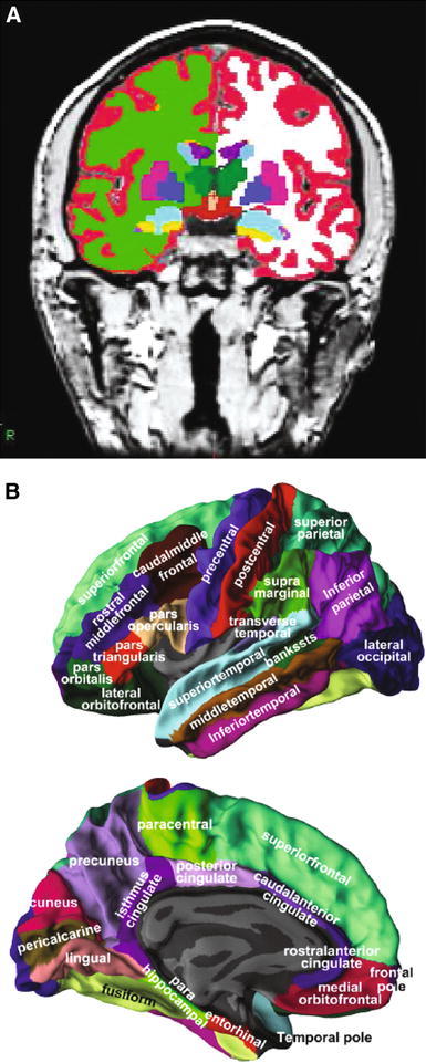
Representations of ROIs included as candidate input variables in the multivariate OPLS model. a Coronal view of a T1-weighted MPRAGE image displaying the regional volumes. b Lateral and medial views of the grey matter surface illustrating the 34 regional cortical thickness measures
Normalization
We wished to compare the effect of different normalisation approaches on multivariate analysis to determine which gave the best discriminant and predictive performance. To this end we normalised the various MRI measures in a series of ways. All sets of regional MRI measures from each subject were considered in their raw form and also normalized by the subject’s intracranial volume. Further, the cortical thickness measures and the surface area measures from each subject were also normalized by the subject’s average global cortical thickness and the subject’s total surface area respectively.
Statistical Analysis
MRI measures were analyzed using OPLS (Bylesjo et al. 2007; Trygg and Wold 2002; Rantalainen et al. 2006; Westman et al. 2011c, 2010; Wiklund et al. 2008), a supervised multivariate data analysis method included in the software package SIMCA (Umetrics AB, Umea, Sweden). A very similar method, partial least squares to latent structures (PLS) has previously been used in several studies to analyze MR-data (Levine et al. 2008; McIntosh and Lobaugh 2004; Oberg et al. 2008; Westman et al. 2009, 2007). OPLS and PLS give the same predictive accuracy, but the advantage of OPLS is that the model created to compare groups is rotated, which means that the information related to class separation is found in the first component of the model, the predictive component. The other orthogonal components in the model, if any, relate to variation in the data not connected to class separation. Focusing the information related to class separation on the first component makes data interpretation easier (Wiklund et al. 2008). There are also many similarities between linear support vector machine (SVM) and OPLS. Both methods can handle datasets with more dimensions than samples. Linear SVM weights illustrate the importance of the variables for the classification in descending order in the same way as the loadings plots do for OPLS. The unique property of OPLS when compared to other linear regression methods is its ability to separate the modeling of correlated variation from structured noise (uncorrelated variation). The structured noise is defined as orthogonal variation in Y. At the same time the model maximizes the covariance between X and Y.
Pre-processing was performed using mean centring and unit variance scaling. Mean centring improves the interpretability of the data, by subtracting the variable average from the data. By doing so the data set is repositioned around the origin. Large variance variables are more likely to be expressed in modeling than low variance variables. Consequently, unit variance scaling was selected to scale the data appropriately. This scaling method calculates the standard deviation of each variable. The inverse standard deviation is used as a scaling weight for each MR-measure.
The results from the OPLS analysis are visualized in a scatter plot by plotting the predictive component, which contains the information related to class separation. Components are vectors, which are linear combinations of partial vectors and are dominated by the input variables (x), in this case the regional MRI output. Each point in the scatter plot represents one individual subject.
Each model receives a Q2(Y) value that describes its statistical significance for separating groups. Q2(Y) values >0.05 are regarded as statistically significant (Umetrics 2008), where
| 1 |
where PRESS (predictive residual sum of squares) = Σ(yactual − ypredicted)2 and SSY is the total variation of the Y matrix after scaling and mean centring (Eriksson et al. 2006). Q2(Y) is the fraction of the total variation of the Ys (expected class values) that can be predicted by a component according to cross validation (CV). CV is a statistical method for validating a predictive model which involves building a number of parallel models. These models differ from each other by leaving out a part of the data set each time. The data omitted is then predicted by the respective model. In this study we used seven fold CV, which means that 1/7th of the data is omitted for each CV round. Data is omitted once and only once.
Variables can be plotted according to their importance for the separation of groups. The plot shows the MRI measures and their corresponding jack-knifed confidence intervals. Jack-knifing is used to estimate the bias and standard error. Measures with confidence intervals that include zero have low reliability (Wiklund et al. 2008). Covariance is plotted on the y-axis, where
| 2 |
where t is the transpose of the score vector t in the OPLS model, i is the centered variable in the data matrix X and N is the number of variables (Wiklund et al. 2008). A measure with high covariance is more likely to have an impact on group separation than a variable with low covariance. MRI measures below zero in the scatter plot have lower values in AD subjects compared to CTL subjects, while MRI measures above zero are higher in AD subjects compared to CTL subjects in the model.
Altogether eight types of regional MRI measures were used (cortical thickness, cortical volumes, subcortical volumes surface area, mean curvature, gaussian curvature, folding index and curvature index), resulting in a total of 259 variables to be used for OPLS analysis (Table 2). A series of OPLS models were created for comparing the CTL versus AD groups. For each of the eight types of measures, both raw measures and measures normalized by intracranial volume (ICV) were used in these models. In addition cortical thickness measures were also normalised by mean cortical thickness and surface area measures by total surface area. Subsequently hierarchical models consisting of combinations of two or three sets of regional measures were also created (for example raw cortical thickness measures and raw subcortical volumes, or cortical thickness measures normalised by intracranial volume and subcortical volumes normalised by intracranial volume). Feature selection was not used other than excluding measures which resulted in non-significant models. Excluding specific regions from the models might make the models less representative and structural features measured from a limited set of pre-defined regions might not be able to reflect the pattern of structural abnormalities in their entirety (Zhang et al. 2011). Further, Cuignet et al. (2011) showed that feature selection does not improve the classification but it does increase the computational time. Another recent paper investigated the effect of feature selection (Chu et al. 2012) and they concluded that feature selection improves the results particularly for small cohorts but it does not seem to have a great affect on larger samples. We have a much larger sample than the largest sample used in this latter study.
The MCI subjects were also assessed against the best CTL versus AD models to investigate how well the model could predict conversion at 18 month follow-up from baseline. Sensitivity, specificity, accuracy and area under the receiver operating characteristic curve (AUC) of the different models were calculated from the cross-validated prediction values of the OPLS models. Areas under the receiver operating characteristic curve were compared by using the method of Hanley and McNeil (1983; McEvoy et al. 2011), p-values <0.05 after correcting for multiple comparisons using Bonferroni correction were considered statistically significant.
The two-way Student t test with Bonferroni correction (p-values > 0.05 considered significant) was used for univariate analysis to investigate the effect of normalization of single regional measures (Tables 6; 7).
Table 6.
Univariate analysis of subcortical volumes using different normalization approaches for AD versus CTL
| Subcortical measures | Subcortical volumes | |
|---|---|---|
| Normalization | Raw | ICV |
| Third ventricle | ns | p < 0.01 |
| Fourth ventricle | ns | ns |
| Inferior lateral ventricle | p < 0.00001 | p < 0.00001 |
| Lateral ventricle | p < 0.00001 | p < 0.00001 |
| Cerebrospinal fluid (CSF) | P < 0.001 | p < 0.00001 |
| Accumbens | p < 0.00001 | p < 0.00001 |
| Amygdala | p < 0.00001 | p < 0.00001 |
| Brainstem | ns | p < 0.00001 |
| Caudate | ns | ns |
| Cerebellum cortex | ns | ns |
| Cerebellum white matter | ns | ns |
| Corpus callosum anterior | ns | ns |
| Corpus callosum central | p < 0.001 | p < 0.001 |
| Corpus callosum midanterior | p < 0.01 | p < 0.001 |
| Corpus callosum midposterior | p < 0.001 | p < 0.00001 |
| Corpus callosum posterior | ns | p < 0.01 |
| Hippocampus | p < 0.00001 | p < 0.00001 |
| Putamen | ns | ns |
| Pallidum | ns | ns |
| Thalamus proper | ns | ns |
| Ventral diencephalon (DC) | p < 0.001 | p < 0.00001 |
Bold values illustrate that there are differences in normalization method
AD = Alzheimer’s disease, CTL = healthy control, ICV = intra cranial volume and raw = not normalized. Two-way Student t test with Bonferroni correction is used for univariate analysis. P-values <0.05 considered significant after Bonferroni correction
Table 7.
Univariate analysis of cortical thickness and volumes using different normalization approaches for AD versus CTL
| Cortical measures | Cortical thickness | Cortical volume | |||
|---|---|---|---|---|---|
| Normalization | Raw | ICV | Mean CT | Raw | ICV |
| Banks of superior temporal sulcus | p < 0.00001 | p < 0.00001 | p < 0.00001 | p < 0.00001 | p < 0.00001 |
| Caudal anterior cingulate | ns | ns | p < 0.00001 | Ns | ns |
| Caudal middle frontal gyrus | p < 0.00001 | p < 0.001 | ns | Ns | ns |
| Cuneus cortex | ns | ns | p < 0.00001 | Ns | ns |
| Entorhinal cortex | p < 0.00001 | p < 0.00001 | p < 0.00001 | p < 0.00001 | p < 0.00001 |
| Fusiform gyrus | p < 0.00001 | p < 0.00001 | p < 0.00001 | p < 0.00001 | p < 0.00001 |
| Inferior parietal cortex | p < 0.00001 | p < 0.00001 | p < 0.00001 | p < 0.00001 | p < 0.00001 |
| Inferior temporal gyrus | p < 0.00001 | p < 0.00001 | p < 0.00001 | p < 0.00001 | p < 0.00001 |
| Isthmus of cingulate cortex | p < 0.00001 | p < 0.001 | ns | p < 0.001 | p < 0.00001 |
| Lateral occipital cortex | p < 0.00001 | p < 0.05 | ns | Ns | p < 0.001 |
| Lateral orbitofronral cortex | p < 0.00001 | ns | ns | Ns | p < 0.05 |
| Lingual gyrus | p < 0.00001 | ns | p < 0.01 | p < 0.05 | p < 0.01 |
| Medial orbitalfrontal cortex | p < 0.00001 | p < 0.01 | Ns | p < 0.01 | p < 0.00001 |
| Middle temporal gyrus | p < 0.00001 | p < 0.00001 | p < 0.00001 | p < 0.00001 | p < 0.00001 |
| Parahippocampal gyrus | p < 0.00001 | p < 0.00001 | p < 0.00001 | p < 0.00001 | p < 0.00001 |
| Paracentral sulcus | ns | ns | p < 0.00001 | Ns | ns |
| Frontal operculum | p < 0.00001 | ns | p < 0.00001 | Ns | ns |
| Orbital operculum | p < 0.00001 | ns | ns | p < 0.05 | p < 0.01 |
| Triangular part of inferior frontal gyrus | p < 0.00001 | ns | p < 0.01 | p < 0.01 | p < 0.001 |
| Pericalcarine cortex | ns | ns | p < 0.00001 | ||
| Postcentral gyrus | p < 0.01 | ns | p < 0.00001 | p < 0.01 | |
| Posterior cingulate cortex | p < 0.001 | ns | p < 0.01 | p < 0.01 | p < 0.00001 |
| Precentral gyrus | p < 0.001 | ns | |||
| Precuneus cortex | p < 0.00001 | p < 0.00001 | p < 0.00001 | p < 0.00001 | |
| Rostral anterior cingulate cortex | ns | ns | p < 0.01 | Ns | ns |
| Rostral middle frontal gyrus | p < 0.00001 | p < 0.001 | ns | p < 0.001 | p < 0.00001 |
| Superior frontal gyrus | p < 0.00001 | p < 0.01 | ns | p < 0.01 | p < 0.00001 |
| Superior parietal gyrus | p < 0.00001 | p < 0.01 | ns | p < 0.01 | p < 0.00001 |
| Superior temporal gyrus | p < 0.00001 | p < 0.00001 | ns | p < 0.00001 | p < 0.00001 |
| Supramarginal gyrus | p < 0.00001 | p < 0.00001 | ns | p < 0.00001 | p < 0.00001 |
| Frontal pole | p < 0.001 | ns | ns | p < 0.001 | p < 0.001 |
| Temporal pole | p < 0.00001 | p < 0.00001 | ns | p < 0.00001 | p < 0.00001 |
| Transverse temporal cortex | ns | ns | ns | Ns | p < 0.01 |
| Insular | p < 0.00001 | ns | ns | Ns | p < 0.0001 |
Bold values illustrate that there are differences in normalization method
AD = Alzheimer’s disease, CTL = healthy control, ICV = intra cranial volume, Raw = not normalized and mean CT = normalized by mean cortical thickness. Two-way Student t test with Bonferroni correction is used for univariate analysis
Results
OPLS models were created using CTL versus AD data for all eight types of regional MRI measures (cortical thickness, cortical volume, subcortical volume, surface area, mean curvature, gaussian curvature, folding index and curvature index) for both raw data and normalized data. Hierarchical models were also created using up to three types of different regional MRI measures. No feature selection was performed for any of the eight different types of measures, meaning all data was included.
Modeling and quality parameters are only shown for the statistically significant single measure models and the most robust [highest Q2(Y)] hierarchical models (Table 3: raw data, Table 4: ICV normalized data, Table 5: data normalized by total surface area, average cortical thickness and mixed models including both normalized and raw data).
Table 3.
Raw data (data not normalized)

|
Q2(Y) = predictive ability of model and AUC = area under the curve. Confidence interval within parentheses. Thick line separating models (within the table content) means that the block of models are significantly different in AUC compared to the other models in that category of normalization method and number of input measures
* Significant difference in AUC between raw data versus normalized with intra cranial volume. ** Significant difference in AUC between raw data and normalized with intra cranial volume and raw data versus normalized with mean cortical thickness. P-values <0.05 considered significant after Bonferroni correction
Table 4.
Data normalized by intra cranial volume
|
Q2(Y) = predictive ability of model and AUC = area under the curve. Confidence interval within parentheses. Thick line separating models (within the table content) means that the block of models are significantly different in AUC compared to the other models in that category of normalization method and number of input measures
* Significant difference in AUC between raw data versus normalized with intra cranial volume. P-values <0.05 considered significant after Bonferroni correction
Table 5.
Other normalization models
| Model | Q2(Y) | Accuracy | Sensitivity | Specificity | AUC | |||
|---|---|---|---|---|---|---|---|---|
| CT (normalized with average CT) | 0.476 | 83.7 | (80.0-87.0) | 83.0 | (76.8-87.6) | 84.8 | (79.6-88.9) | 0.912** |
| SA (normalized with total SA) | 0.169 | 69.2 | (64.6-73.4) | 71.1 | (64.3-77.4) | 67.6 | (61.2-73.3) | 0.744 |
| Hierarchial model | ||||||||
| SV + CT* | 0.603 | 89.3 | (86.0-92.0) | 87.2 | (81.6-91.2) | 91.1 | (86.7-94.2) | 0.951 |
| CV + CT* | 0.592 | 88.4 | (84.9-91.1) | 86.6 | (81.0-90.8) | 89.8 | (85.1-93.1) | 0.951 |
| Hierarchial model | ||||||||
| SV + CV + CT* | 0.626 | 91.5 | (88.4-93.8) | 89.8 | (86.5-92.4) | 92.9 | (88.8-95.6) | 0.960 |
Q2(Y) = predictive ability of model, CV cortical volume, SV subcortical volume, CT cortical thickness, SA surface area and AUC area under the curve. Confidence interval within parentheses. * Mixed model = SV and CV normalized by ICV with raw CT data. ** Significant difference in AUC between raw data and normalized with mean cortical thickness. P-values <0.05 considered significant after Bonferroni correction
Figure 2 shows the variables of importance for the three most robust single measure models [subcortical volumes (ICV normalized), cortical volumes (ICV normalized) and cortical thickness measures (raw data)]. Variables of greatest importance for the separation between groups were as expected the medial temporal lobe structures such as hippocampus, amygdala and entorhinal cortex. To illustrate the effect of normalization approaches on single measures univariate analysis was performed for subcortical volumes (Table 6), cortical volumes and cortical thickness measures (Table 7). As can be observed in Tables 6 and 7, normalizing volumes with ICV and raw cortical thickness measures gave the best results.
Fig. 2.
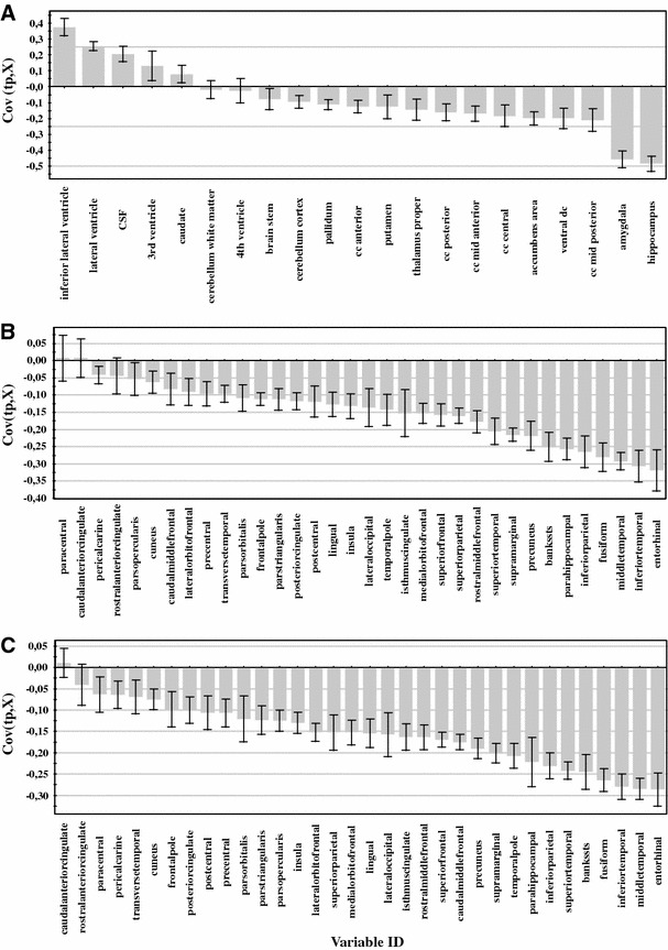
Variables of importance for the separation between CTL versus AD. a subcortical volumes (normalized by intra cranial volume) b cortical gray matter volumes (normalized by intra cranial volume) c cortical thickness (raw data). Measures above zero have a larger value in AD compared to controls and measures below zero have a lower value in AD compared to controls. A measure with a high covariance is more likely to have an impact on group separation than a measure with a low covariance. Measures with jack knifed confidence intervals that include zero have low reliability
AD Classification and MCI Conversion
The results from the different models used for AD classification can be observed in Tables 3, 4, 5. The AUC values for the different models were compared using the method of Hanley and McNeil and p-values <0.05 after Bonferroni correction for multiple comparisons were considered statistically significant. Only five out of the eight single measure models gave significant results for both raw and normalized data. Gaussian curvature, folding index and curvature index were therefore excluded from further analysis. Out of the five remaining measures the best results were obtained from the cortical thickness, cortical volume and subcortical volume measures (these measures were significantly different from surface area and mean curvature for both raw data and data normalized to ICV). Using raw data the best discrimination was obtained for cortical thickness measures with an accuracy of 85.2 % (significantly different from cortical and subcortical volumes) and for data normalized by ICV the best discrimination was obtained from the cortical volumes with an accuracy of 83.5 % (significantly different from cortical thickness and subcortical volumes). Looking at the normalization approaches for the single measures, a significantly better result was obtained for the cortical thickness measures when the data was not normalized, compared to normalization with ICV and mean cortical thickness (85.2 % compared to 83.5 and 83.7 % respectively). For cortical volumes it was significantly better to normalize with ICV than to use raw data (83.5 % compared to 81.8 %). For the other measures normalization did not have an effect. Figure 3 shows the scatter plots for the top three single measures (raw data cortical thickness and ICV normalized cortical and subcortical volumes) illustrating the separation between the AD and CTL groups.
Fig. 3.
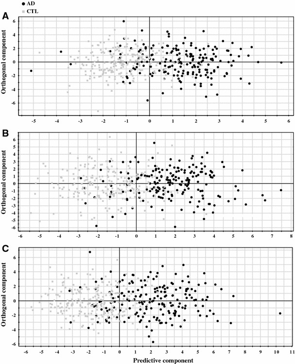
Scatter plots illustrating the separation between CTL versus AD. a subcortical volumes (normalized by intra cranial volume) b cortical gray matter volumes (normalized by intra cranial volume) c cortical thickness (raw data). The scatter plots visualise group separation and the predictability of three different AD versus CTL models. Each black circle represents an AD subject and each gray square a control subject. Control subjects to the right of zero and AD subjects to the left of zero are falsely predicted
For the hierarchical models containing a combination of two different measures the best models were the combination of subcortical volumes with either cortical thickness or cortical volumes for both raw data and ICV normalization (Raw data: subcortical volumes + cortical thickness = 89.8 %, subcortical volumes + cortical volumes = 88.6 %. ICV normalized data: subcortical volumes + cortical volumes = 89.8 %, subcortical volumes + cortical thickness = 88.4 %). There seemed to be no effect of normalization approaches for the most accurate and robust models combining two different measures. No effect of normalization approach was observed either for the models containing three different measures.
Combining three different measures did not significantly affect the prediction accuracy compared to using two different measures. Only the three best models are shown using the combination of cortical thickness, cortical volume and subcortical volumes. However, the best overall prediction accuracy was obtained using this combination with raw cortical thickness data and volumes normalized to ICV (91.5 %).
Finally the best AD versus CTL models containing the measures cortical thickness, cortical volumes and subcortical volumes were used to predict conversion at 18 month follow-up. Out of 287 MCI subjects 87 had converted to AD at follow up. Similar results were observed for the MCI predictions as for the models discriminating between AD patients and cognitively normal subjects (Table 8). The best results were obtained with a hierarchical model of two sets of measures when subcortical volumes were combined with either cortical volumes or cortical thickness. Combining the three measures did not improve the predictions and normalization approach did not seem to significantly affect the results either. The best results were obtained from the two models combining cortical thickness with subcortical volumes (both ICV normalized data and mixed data where the volumes are normalized to ICV and the raw cortical thickness data was used) with 77 % of the MCIc subjects correctly classified.
Table 8.
MCI predictions using the CTL versus AD models as training data
| Raw data | Sensitivity (%) | Specificity (%) | Accuracy (%) | AUC |
|---|---|---|---|---|
| SV + CV | 75.9 | 60.5 | 65.1 | 0.734 |
| SV + CT | 74.7 | 62.5 | 66.2 | 0.746 |
| CV + CT | 67.8 | 69.0 | 68.6 | 0.742 |
| SV + CV + CT | 75.9 | 64.0 | 67.6 | 0.753 |
| Average | 73.6 | 64.0 | 66.9 | 0.744 |
| ICV normalized | ||||
| SV + CT | 77.0 | 65.0 | 68.6 | 0.739 |
| SV + CV | 75.9 | 60.5 | 65.1 | 0.729 |
| CV + CT | 68.9 | 67.0 | 67.6 | 0.736 |
| SV + CV + CT | 73.5 | 64.0 | 66.9 | 0.743 |
| Average | 73.8 | 64.1 | 67.1 | 0.737 |
| Mixed models* | ||||
| SV + CT | 77.0 | 64.5 | 68.3 | 0.749 |
| CV + CT | 70.1 | 67.0 | 67.9 | 0.743 |
| SV + CV + CT | 75.9 | 66.5 | 69.3 | 0.748 |
| Average | 74.3 | 66.0 | 68.5 | 0.747 |
CV cortical volume, SV subcortical volume, CT cortical thickness, AD Alzheimer’s disease, CTL healthy control, MCI mild cognitive impairment and ICV intra cranial volume. 287 MCI subjects are predicted on to the different AD versus CTL models, 87 MCI converters and 200 MCI stable. Sensitivity = MCI converters predicted as AD and specificity = MCI stable predicted as CTL. * Mixed model = SV and CV normalized by ICV and raw CT data
Discussion
The Freesurfer pipeline has been utilized in a number of studies for AD classification and predicting MCI conversion (Cui et al. 2011; Cuingnet et al. 2011; McEvoy et al. 2009, 2011; Westman et al. 2011a, b), but the complete range of measures which can be obtained have not yet been fully explored.
Normalization
The way in which different regional measures such as volumes and cortical thickness should be normalized is very important. Previous studies (Barnes et al. 2010; Cui et al. 2011; Farias et al. 2011; Fjell et al. 2009; Walhovd et al. 2011; Westman et al. 2011b) have utilized different approaches which can make results difficult to compare. The results from the present study indicate that cortical thickness measures should not be normalized, while volumes should probably be normalized to ICV. Normalizing cortical volumes improved the classification accuracy while normalizing subcortical volumes did not show any statistically significant improvement using the single measure OPLS multivariate models. Further, looking at the single regions (Tables 6, 7), it seems that normalizing the volumes results in the largest differences while using the raw data for cortical thickness yields the best results. When combining the different measures in multivariate models the normalization effect disappears. A potential explanation for this could be that the use of multiple regional measures provides enough anatomical information about the brain atrophy pattern such that multivariate models are robust enough to handle the variation caused by different normalization approaches. In a recent paper, the consistency of volumetric measures derived by FreeSurfer was investigated in five different cohorts (a total of 883 subjects) (Walhovd et al. 2011). This study normalized regional volume measurements by ICV as we propose here. They concluded that ICV normalization is the most commonly used normalization approach in the literature. However, it has also been stated that normalizing to ICV is unlikely to be adequate due to the non-linear relationship between volumes and ICV which was found in a sample of 78 healthy controls (Barnes et al. 2010). Another recent study also stated that normalizing volumes to ICV is inadequate due to the fact that the maximal brain size seems to be an important predictor of cognition in old age, independent of brain pathology (Farias et al. 2011). By normalizing to ICV, the authors claim that investigators may overlook the effect of ICV itself. Especially in longitudinal studies, ICV may be an important variable in itself for quantifying the effect of brain reserve (Farias et al. 2011). Reviewing the literature regarding normalizing cortical thickness, there seems to be a common agreement that these measures should not be normalized (Fjell et al. 2009). This is also confirmed in the present study, where normalized cortical thickness measures gave significantly lower prediction accuracies regardless of normalization approach (mean thickness or ICV).
Previous studies have drawn different conclusions on the best normalization approach to adopt for regional MRI measures. However, we feel fairly confident to say from the results of the present study and results from previous studies that cortical thickness should not be normalized. Normalizing volumes seems to be a more complicated issue however. We believe that considering single regions, the best approach is to normalize to ICV. Even though the relationship between ICV and volumes may not be linear and the effect of ICV itself may be removed if data is normalized, we still believe this may be the best approach to take. This is due to the fact that changes in neurodegenerative disorders are relatively small and could be overlooked if data is not normalized. When we consider multivariate models containing multiple brain regions the normalization approach does not seem to be that important. This need to be further validated in larger studies.
AD Classification and MCI Conversion
Previous studies have utilized different types of regional MRI measures for AD classification and to predict MCI conversion (Cui et al. 2011; Cuingnet et al. 2011; McEvoy et al. 2009, 2011; Westman et al. 2011a, b). Whole brain volume, regional volumes and cortical thickness measures (volumes normalized to ICV and raw cortical thickness data) were included in a recent study (McEvoy et al. 2011). This study obtained a prediction accuracy of 90.4 % between AD and CTL using a smaller sample from the same cohort as in this study (ADNI). This is very similar to the best accuracies obtain in this study ranging between 89.3 and 91.5 %. Data from the ADNI cohort was also utilized in another study, which included cortical thickness measures and regional cortical and subcortical volumes (data not normalized), to train a SVM classifier using AD and CTL data (Cui et al. 2011). The MCI subjects were then used as a test set (in the same way as in the present study) to predict future conversion at baseline. Using the measures mentioned above 57.1 % of the MCIc and 65.5 % of MCIs were correctly classified, compared to 77 and 65.0 % respectively in the present study.
Other recent studies which did not use Freesurfer as input for multivariate analysis have also found results in line with ours. SVM has been successfully utilized with voxel based input with accuracies up to 90.8 % (Chu et al. 2012; Liu et al. 2012). Our results are also in line with those of Zhang et al. (2011) who found a classification accuracy of 93.2 % when combining ROI based MRI measures with FDG-PET and CSF.
Conclusion
Automated MRI image analysis pipelines can be used as input for multivariate data analysis and machine learning techniques, but there is also the option of using raw images as the input to similar multivariate or machine learning approaches. One of the major advantages of automated analysis pipelines is their use of a number of predefined regions which are easy to interpret and have a defined biological meaning. These have greater face validity as a biomarker of disease than a complex pattern of individual voxels across the brain (McEvoy et al. 2011). This study demonstrates that combining raw cortical thickness measures with subcortical volumes normalized by intracranial volume gives the best prediction accuracy for separating AD subjects from cognitively normal subjects. Adding further measures did not significantly improve the classification accuracy, most likely because these additional measures are also derived from the same regions as the cortical thickness measures and provide similar information. Further, normalization approach does not seem to have such a great effect as we initially hypothesized. We do however believe that volumes should be normalized by ICV and that raw cortical thickness data should be used, especially when looking at single regions or measures. This need to be further validated in alternative cohorts. Finally, the combination of cortical thickness measures with subcortical volumes shows potential for prospectively predicting future conversion to AD from baseline. We believe this is a sensible approach using MRI patterns as a biomarker of disease. Combining this approach with other biomarkers such as CSF markers (Westman et al. 2012) and PET markers is likely to further improve AD classification and MCI conversion accuracy. This will hopefully lead to improved tools to aid AD diagnosis and allow targeting of the right populations for clinical trials.
Acknowledgments
Data collection and sharing for this project was funded by the Alzheimer’s disease Neuroimaging Initiative (ADNI) (National Institutes of Health Grant U01 AG024904). ADNI is funded by the National Institute on Aging, the National Institute of Biomedical Imaging and Bioengineering, and through generous contributions from the following: Abbott, AstraZeneca AB, Bayer Schering Pharma AG, Bristol-Myers Squibb, Eisai Global Clinical Development, Elan Corporation, Genentech, GE Healthcare, GlaxoSmithKline, Innogenetics, Johnson and Johnson, Eli Lilly and Co., Medpace, Inc., Merck and Co., Inc., Novartis AG, Pfizer Inc, F. Hoffman-La Roche, Schering-Plough, Synarc, Inc., as well as non-profit partners the Alzheimer’s Association and Alzheimer’s Drug Discovery Foundation, with participation from the U.S. Food and Drug Administration. Private sector contributions to ADNI are facilitated by the Foundation for the National Institutes of Health (www.fnih.org). The grantee organization is the Northern California Institute for Research and Education, and the study is coordinated by the Alzheimer’s disease Cooperative Study at the University of California, San Diego. ADNI data are disseminated by the Laboratory for Neuro Imaging at the University of California, Los Angeles. This research was also supported by NIH Grants P30 AG010129, K01 AG030514, and the Dana Foundation.Also thanks to the Strategic Research Programme in Neuroscience at Karolinska Institutet (StratNeuro), Hjärnfonden and Swedish Brain Power. Andrew Simmons and Eric Westman were supported by funds from the NIHR Biomedical Research Centre for Mental Health, at the South London and Maudsley NHS Foundation Trust and Institute of Psychiatry, Kings College London.
Open Access
This article is distributed under the terms of the Creative Commons Attribution License which permits any use, distribution, and reproduction in any medium, provided the original author(s) and the source are credited.
Footnotes
This study is conducted for the Alzheimer’s Disease Neuroimaging Initiative. Data used in preparation of this article were obtained from the Alzheimer’s disease Neuroimaging Initiative (ADNI) database (www.loni.ucla.edu/ADNI). As such, the investigators within the ADNI contributed to the design and implementation of ADNI and/or provided data but did not participate in analysis or writing of this report. ADNI investigators include (complete listing available at http://adni.loni.ucla.edu/wp-content/uploads/how_to_apply/ADNI_Authorship_List.pdf).
References
- Barnes J, Ridgway GR, Bartlett J, Henley SM, Lehmann M, Hobbs N, Clarkson MJ, MacManus DG, Ourselin S, Fox NC. Head size, age and gender adjustment in MRI studies: a necessary nuisance? Neuroimage. 2010;53:1244–1255. doi: 10.1016/j.neuroimage.2010.06.025. [DOI] [PubMed] [Google Scholar]
- Braak H, Braak E. Neuropathological stageing of Alzheimer-related changes. Acta Neuropathol. 1991;82:239–259. doi: 10.1007/BF00308809. [DOI] [PubMed] [Google Scholar]
- Brookmeyer R, Johnson E, Ziegler-Graham K, Arrighi HM. Forecasting the global burden of Alzheimer’s disease. Alzheimer’s Dement. 2007;3:186–191. doi: 10.1016/j.jalz.2007.04.381. [DOI] [PubMed] [Google Scholar]
- Bylesjo M, Eriksson D, Kusano M, Moritz T, Trygg J. Data integration in plant biology: the O2PLS method for combined modeling of transcript and metabolite data. Plant J. 2007;52:1181–1191. doi: 10.1111/j.1365-313X.2007.03293.x. [DOI] [PubMed] [Google Scholar]
- Chu C, Hsu A-L, Chou K-H, Bandettini P, Lin C. Does feature selection improve classification accuracy? Impact of sample size and feature selection on classification using anatomical magnetic resonance images. Neuroimage. 2012;60:59–70. doi: 10.1016/j.neuroimage.2011.11.066. [DOI] [PubMed] [Google Scholar]
- Cui Y, Liu B, Luo S, Zhen X, Fan M, Liu T, Zhu W, Park M, Jiang T, Jin JS, the Alzheimer’s Disease Neuroimaging, I Identification of conversion from mild cognitive impairment to Alzheimer’s disease using multivariate predictors. PLoS ONE. 2011;6:e21896. doi: 10.1371/journal.pone.0021896. [DOI] [PMC free article] [PubMed] [Google Scholar]
- Cuingnet R, Gerardin E, Tessieras J, Auzias G, Lehericy S, Habert MO, Chupin M, Benali H, Colliot O. Automatic classification of patients with Alzheimer’s disease from structural MRI: a comparison of ten methods using the ADNI database. Neuroimage. 2011;56:766–781. doi: 10.1016/j.neuroimage.2010.06.013. [DOI] [PubMed] [Google Scholar]
- Dale AM, Sereno MI. Improved localizadon of cortical activity by combining EEG and MEG with MRI cortical surface reconstruction: a linear approach. J Cogn Neurosci. 1993;5:162–176. doi: 10.1162/jocn.1993.5.2.162. [DOI] [PubMed] [Google Scholar]
- Dale AM, Fischl B, Sereno MI. Cortical surface-based analysis. I. Segmentation and surface reconstruction. Neuroimage. 1999;9:179–194. doi: 10.1006/nimg.1998.0395. [DOI] [PubMed] [Google Scholar]
- Desikan RS, Ségonne F, Fischl B, Quinn BT, Dickerson BC, Blacker D, Buckner RL, Dale AM, Maguire RP, Hyman BT, Albert MS, Killiany RJ. An automated labeling system for subdividing the human cerebral cortex on MRI scans into gyral based regions of interest. Neuroimage. 2006;31:968–980. doi: 10.1016/j.neuroimage.2006.01.021. [DOI] [PubMed] [Google Scholar]
- Dubois B, Feldman HH, Jacova C, DeKosky ST, Barberger-Gateau P, Cummings J, Delacourte A, Galasko D, Gauthier S, Jicha G, Meguro K, O’Brien J, Pasquier F, Robert P, Rossor M, Salloway S, Stern Y, Visser PJ, Scheltens P. Research criteria for the diagnosis of Alzheimer’s disease: revising the NINCDS-ADRDA criteria. Lancet Neurol. 2007;6:734–746. doi: 10.1016/S1474-4422(07)70178-3. [DOI] [PubMed] [Google Scholar]
- Eriksson L, Johansson E, Kettaneh-Wold N, Trygg J, Wiksröm C, Wold S. Multi- and megavariate data analysis (Part I-Basics and principals and applications) 2. Umeå: Umetrics AB; 2006. [Google Scholar]
- Farias ST, Mungas D, Reed B, Carmichael O, Beckett L, Harvey D, Olichney J, Simmons A, Decarli C. Maximal brain size remains an important predictor of cognition in old age, independent of current brain pathology. Neurobiol Aging. 2011;33(8):1758–1768. doi: 10.1016/j.neurobiolaging.2011.03.017. [DOI] [PMC free article] [PubMed] [Google Scholar]
- Fischl B, Dale AM. Measuring the thickness of the human cerebral cortex from magnetic resonance images. Proc Natl Acad Sci USA. 2000;97:11050–11055. doi: 10.1073/pnas.200033797. [DOI] [PMC free article] [PubMed] [Google Scholar]
- Fischl B, Sereno MI, Tootell RB, Dale AM. High-resolution intersubject averaging and a coordinate system for the cortical surface. Hum Brain Mapp. 1999;8:272–284. doi: 10.1002/(SICI)1097-0193(1999)8:4<272::AID-HBM10>3.0.CO;2-4. [DOI] [PMC free article] [PubMed] [Google Scholar]
- Fischl B, Liu A, Dale AM. Automated manifold surgery: constructing geometrically accurate and topologically correct models of the human cerebral cortex. IEEE Trans Med Imaging. 2001;20:70–80. doi: 10.1109/42.906426. [DOI] [PubMed] [Google Scholar]
- Fischl B, Salat DH, Busa E, Albert M, Dieterich M, Haselgrove C, van der Kouwe A, Killiany R, Kennedy D, Klaveness S, Montillo A, Makris N, Rosen B, Dale AM. Whole brain segmentation: automated labeling of neuroanatomical structures in the human brain. Neuron. 2002;33:341–355. doi: 10.1016/S0896-6273(02)00569-X. [DOI] [PubMed] [Google Scholar]
- Fischl B, Salat DH, van der Kouwe AJ, Makris N, Segonne F, Quinn BT, Dale AM. Sequence-independent segmentation of magnetic resonance images. Neuroimage. 2004;23(Suppl 1):S69–S84. doi: 10.1016/j.neuroimage.2004.07.016. [DOI] [PubMed] [Google Scholar]
- Fischl B, van der Kouwe A, Destrieux C, Halgren E, Segonne F, Salat DH, Busa E, Seidman LJ, Goldstein J, Kennedy D, Caviness V, Makris N, Rosen B, Dale AM. Automatically parcellating the human cerebral cortex. Cereb Cortex. 2004;14:11–22. doi: 10.1093/cercor/bhg087. [DOI] [PubMed] [Google Scholar]
- Fjell AM, Westlye LT, Amlien I, Espeseth T, Reinvang I, Raz N, Agartz I, Salat DH, Greve DN, Fischl B, Dale AM, Walhovd KB. High consistency of regional cortical thinning in aging across multiple samples. Cereb Cortex. 2009;19:2001–2012. doi: 10.1093/cercor/bhn232. [DOI] [PMC free article] [PubMed] [Google Scholar]
- Fox NC, Warrington EK, Freeborough PA, Hartikainen P, Kennedy AM, Stevens JM, Rossor MN. Presymptomatic hippocampal atrophy in Alzheimer’s disease. A longitudinal MRI study. Brain. 1996;119(Pt 6):2001–2007. doi: 10.1093/brain/119.6.2001. [DOI] [PubMed] [Google Scholar]
- Glenner GG, Wong CW. Alzheimer’s disease: initial report of the purification and characterization of a novel cerebrovascular amyloid protein. Biochem Biophys Res Commun. 1984;120:885–890. doi: 10.1016/S0006-291X(84)80190-4. [DOI] [PubMed] [Google Scholar]
- Goedert M, Spillantini MG, Crowther RA. Tau proteins and neurofibrillary degeneration. Brain Pathol. 1991;1:279–286. doi: 10.1111/j.1750-3639.1991.tb00671.x. [DOI] [PubMed] [Google Scholar]
- Hanley J, McNeil B. A method of comparing the areas under receiver operating characteristic curves derived from the same cases. Radiology. 1983;148:839–843. doi: 10.1148/radiology.148.3.6878708. [DOI] [PubMed] [Google Scholar]
- Jack CR, Jr, Petersen RC, O’Brien PC, Tangalos EG. MR-based hippocampal volumetry in the diagnosis of Alzheimer’s disease. Neurology. 1992;42:183–188. doi: 10.1212/WNL.42.1.183. [DOI] [PubMed] [Google Scholar]
- Jack CR, Jr, Petersen RC, Xu YC, Waring SC, O’Brien PC, Tangalos EG, Smith GE, Ivnik RJ, Kokmen E. Medial temporal atrophy on MRI in normal aging and very mild Alzheimer’s disease. Neurology. 1997;49:786–794. doi: 10.1212/WNL.49.3.786. [DOI] [PMC free article] [PubMed] [Google Scholar]
- Juottonen K, Laakso MP, Partanen K, Soininen H. Comparative MR analysis of the entorhinal cortex and hippocampus in diagnosing Alzheimer disease. AJNR Am J Neuroradiol. 1999;20:139–144. [PubMed] [Google Scholar]
- Levine B, Kovacevic N, Nica EI, Cheung G, Gao F, Schwartz ML, Black SE. The Toronto traumatic brain injury study: injury severity and quantified MRI. Neurology. 2008;70:771–778. doi: 10.1212/01.wnl.0000304108.32283.aa. [DOI] [PubMed] [Google Scholar]
- Li C, Wang J, Gui L, Zheng J, Liu C, Du H. Alterations of whole-brain cortical area and thickness in mild cognitive impairment and Alzheimer’s disease. J Alzheimer’s Dis. 2011;27(2):281–290. doi: 10.3233/JAD-2011-110497. [DOI] [PubMed] [Google Scholar]
- Liu Y, Paajanen T, Westman E, Wahlund LO, Simmons A, Tunnard C, Sobow T, Proitsi P, Powell J, Mecocci P, Tsolaki M, Vellas B, Muehlboeck S, Evans A, Spenger C, Lovestone S, Soininen H. Effect of APOE epsilon4 allele on cortical thicknesses and volumes: the AddNeuroMed study. J Alzheimer’s Dis. 2010;21:947–966. doi: 10.3233/JAD-2010-100201. [DOI] [PubMed] [Google Scholar]
- Liu Y, Paajanen T, Westman E, Zhang Y, Wahlund LO, Simmons A, Tunnard C, Sobow T, Proitsi P, Powell J, Mecocci P, Tsolaki M, Vellas B, Muehlboeck S, Evans A, Spenger C, Lovestone S, Soininen H. APOE epsilon2 allele is associated with larger regional cortical thicknesses and volumes. Dement Geriatr Cogn Disord. 2010;30:229–237. doi: 10.1159/000320136. [DOI] [PubMed] [Google Scholar]
- Liu Y, Paajanen T, Zhang Y, Westman E, Wahlund L-O, Simmons A, Tunnard C, Sobow T, Mecocci P, Tsolaki M, Vellas B, Muehlboeck S, Evans A, Spenger C, Lovestone S, Soininen H. Analysis of regional MRI volumes and thicknesses as predictors of conversion from mild cognitive impairment to Alzheimer’s disease. Neurobiol Aging. 2010;31:1375–1385. doi: 10.1016/j.neurobiolaging.2010.01.022. [DOI] [PubMed] [Google Scholar]
- Liu Y, Paajanen T, Zhang Y, Westman E, Wahlund LO, Simmons A, Tunnard C, Sobow T, Mecocci P, Tsolaki M, Vellas B, Muehlboeck S, Evans A, Spenger C, Lovestone S, Soininen H. Combination analysis of neuropsychological tests and structural MRI measures in differentiating AD, MCI and control groups: The AddNeuroMed study. Neurobiol Aging. 2011;32:1198–1206. doi: 10.1016/j.neurobiolaging.2009.07.008. [DOI] [PubMed] [Google Scholar]
- Liu M, Zhang D, Shen D. Ensemble sparse classification of Alzheimer’s disease. Neuroimage. 2012;60:1106–1116. doi: 10.1016/j.neuroimage.2012.01.055. [DOI] [PMC free article] [PubMed] [Google Scholar]
- Masters CL, Simms G, Weinman NA, Multhaup G, McDonald BL, Beyreuther K. Amyloid plaque core protein in Alzheimer disease and Down syndrome. Proc Natl Acad Sci USA. 1985;82:4245–4249. doi: 10.1073/pnas.82.12.4245. [DOI] [PMC free article] [PubMed] [Google Scholar]
- McEvoy LK, Fennema-Notestine C, Roddey JC, Hagler JDJ, Jr, Holland D, Karow DS, Pung CJ, Brewer JB, Dale AM. Alzheimer disease: quantitative structural neuroimaging for detection and prediction of clinical and structural changes in mild cognitive impairment. Radiology. 2009;251(1):195–205. doi: 10.1148/radiol.2511080924. [DOI] [PMC free article] [PubMed] [Google Scholar]
- McEvoy LK, Holland D, Hagler DJ, Fennema-Notestine C, Brewer JB, Dale AM. Mild cognitive impairment: baseline and longitudinal structural MR imaging measures improve predictive prognosis. Radiology. 2011;259:834–843. doi: 10.1148/radiol.11101975. [DOI] [PMC free article] [PubMed] [Google Scholar]
- McIntosh AR, Lobaugh NJ. Partial least squares analysis of neuroimaging data: applications and advances. Neuroimage. 2004;23:S250–S263. doi: 10.1016/j.neuroimage.2004.07.020. [DOI] [PubMed] [Google Scholar]
- McKhann GM, Knopman DS, Chertkow H, Hyman BT, Jack CR, Jr, Kawas CH, Klunk WE, Koroshetz WJ, Manly JJ, Mayeux R, Mohs RC, Morris JC, Rossor MN, Scheltens P, Carrillo MC, Thies B, Weintraub S, Phelps CH. The diagnosis of dementia due to Alzheimer’s disease: recommendations from the National Institute on Aging-Alzheimer’s Association workgroups on diagnostic guidelines for Alzheimer’s disease. Alzheimer’s Dement. 2011;7:263–269. doi: 10.1016/j.jalz.2011.03.005. [DOI] [PMC free article] [PubMed] [Google Scholar]
- Oberg J, Spenger C, Wang FH, Andersson A, Westman E, Skoglund P, Sunnemark D, Norinder U, Klason T, Wahlund LO, Lindberg M. Age related changes in brain metabolites observed by 1H MRS in APP/PS1 mice. Neurobiol Aging. 2008;29:1423–1433. doi: 10.1016/j.neurobiolaging.2007.03.002. [DOI] [PubMed] [Google Scholar]
- O’Brien JT. Role of imaging techniques in the diagnosis of dementia. Br J Radiol. 2007;80(Spec No 2):S71–S77. doi: 10.1259/bjr/33117326. [DOI] [PubMed] [Google Scholar]
- Rantalainen M, Cloarec O, Beckonert O, Wilson ID, Jackson D, Tonge R, Rowlinson R, Rayner S, Nickson J, Wilkinson RW, Mills JD, Trygg J, Nicholson JK, Holmes E. Statistically integrated metabonomic-proteomic studies on a human prostate cancer xenograft model in mice. J Proteome Res. 2006;5:2642–2655. doi: 10.1021/pr060124w. [DOI] [PubMed] [Google Scholar]
- Ries ML, Carlsson CM, Rowley HA, Sager MA, Gleason CE, Asthana S, Johnson SC. Magnetic resonance imaging characterization of brain structure and function in mild cognitive impairment: a review. J Am Geriatr Soc. 2008;56:920–934. doi: 10.1111/j.1532-5415.2008.01684.x. [DOI] [PMC free article] [PubMed] [Google Scholar]
- Segonne F, Dale AM, Busa E, Glessner M, Salat D, Hahn HK, Fischl B. A hybrid approach to the skull stripping problem in MRI. Neuroimage. 2004;22:1060–1075. doi: 10.1016/j.neuroimage.2004.03.032. [DOI] [PubMed] [Google Scholar]
- Segonne F, Pacheco J, Fischl B. Geometrically accurate topology-correction of cortical surfaces using nonseparating loops. IEEE Trans Med Imaging. 2007;26:518–529. doi: 10.1109/TMI.2006.887364. [DOI] [PubMed] [Google Scholar]
- Simmons A, Westman E, Muehlboeck S, Mecocci P, Vellas B, Tsolaki M, Kloszewska I, Wahlund L-O, Soininen H, Lovestone S, Evans A, Spenger C. MRI measures of Alzheimer's disease and the AddNeuroMed study. Ann NY Acad Sci. 2009;1180:47–55. doi: 10.1111/j.1749-6632.2009.05063.x. [DOI] [PubMed] [Google Scholar]
- Simmons A, Westman E, Muehlboeck S, Mecocci P, Vellas B, Tsolaki M, Kloszewska I, Wahlund L-O, Soininen H, Lovestone S, Evans A, Spenger C, for the AddNeuroMed Consortium (2011) The AddNeuroMed framework for multi-centre MRI assessment of longitudinal changes in Alzheimer’s disease: experience from the first 24 months. Int J Geriatr Psychiatry 26(1):75–82 [DOI] [PubMed]
- Sled JG, Zijdenbos AP, Evans AC. A nonparametric method for automatic correction of intensity nonuniformity in MRI data. IEEE Trans Med Imaging. 1998;17:87–97. doi: 10.1109/42.668698. [DOI] [PubMed] [Google Scholar]
- Thambisetty M, Simmons A, Velayudhan L, Hye A, Campbell J, Zhang Y, Wahlund LO, Westman E, Kinsey A, Guntert A, Proitsi P, Powell J, Causevic M, Killick R, Lunnon K, Lynham S, Broadstock M, Choudhry F, Howlett DR, Williams RJ, Sharp SI, Mitchelmore C, Tunnard C, Leung R, Foy C, O’Brien D, Breen G, Furney SJ, Ward M, Kloszewska I, Mecocci P, Soininen H, Tsolaki M, Vellas B, Hodges A, Murphy DG, Parkins S, Richardson JC, Resnick SM, Ferrucci L, Wong DF, Zhou Y, Muehlboeck S, Evans A, Francis PT, Spenger C, Lovestone S. Association of plasma clusterin concentration with severity, pathology, and progression in Alzheimer disease. Arch Gen Psychiatry. 2010;67:739–748. doi: 10.1001/archgenpsychiatry.2010.78. [DOI] [PMC free article] [PubMed] [Google Scholar]
- Trygg J, Wold S. Orthogonal projections to latent structures (O-PLS) J Chemom. 2002;16:119–128. doi: 10.1002/cem.695. [DOI] [Google Scholar]
- Umetrics (2008) Users guide to SIMCA-P+. http://www.umetrics.com/Content/Document%20Library/Files/UserGuides-Tutorials/SIMCA-P_12_UG.pdf. Accessed 03 Aug 2012
- Walhovd KB, Westlye LT, Amlien I, Espeseth T, Reinvang I, Raz N, Agartz I, Salat DH, Greve DN, Fischl B, Dale AM, Fjell AM. Consistent neuroanatomical age-related volume differences across multiple samples. Neurobiol Aging. 2011;32:916–932. doi: 10.1016/j.neurobiolaging.2009.05.013. [DOI] [PMC free article] [PubMed] [Google Scholar]
- Westman E, Spenger C, Wahlund L-O, Lavebratt C. Carbamazepine treatment recovered low N-acetylaspartate + N-acetylaspartylglutamate (tNAA) levels in the megencephaly mouse BALB/cByJ-Kv1.1mceph/mceph. Neurobiol Dis. 2007;26:221–228. doi: 10.1016/j.nbd.2006.12.012. [DOI] [PubMed] [Google Scholar]
- Westman E, Spenger C, Oberg J, Reyer H, Pahnke J, Wahlund LO. In vivo 1H-magnetic resonance spectroscopy can detect metabolic changes in APP/PS1 mice after donepezil treatment. BMC Neurosci. 2009;10:33. doi: 10.1186/1471-2202-10-33. [DOI] [PMC free article] [PubMed] [Google Scholar]
- Westman E, Wahlund L-O, Foy C, Poppe M, Cooper A, Murphy D, Spenger C, Lovestone S, Simmons A. Combining MRI and MRS to distinguish between Alzheimer’s disease and healthy controls. J Alzheimer’s Dis. 2010;22:171–181. doi: 10.3233/JAD-2010-100168. [DOI] [PubMed] [Google Scholar]
- Westman E, Cavallin L, Muehlboeck JS, Zhang Y, Mecocci P, Vellas B, Tsolaki M, Kloszewska I, Soininen H, Spenger C, Lovestone S, Simmons A, Wahlund LO. Sensitivity and specificity of medial temporal lobe visual ratings and multivariate regional MRI classification in Alzheimer’s disease. PLoS One. 2011;6:e22506. doi: 10.1371/journal.pone.0022506. [DOI] [PMC free article] [PubMed] [Google Scholar]
- Westman E, Simmons A, Muehlboeck JS, Mecocci P, Vellas B, Tsolaki M, Kloszewska I, Soininen H, Weiner MW, Lovestone S, Spenger C, Wahlund LO. AddNeuroMed and ADNI: similar patterns of Alzheimer’s atrophy and automated MRI classification accuracy in Europe and North America. Neuroimage. 2011;58:818–828. doi: 10.1016/j.neuroimage.2011.06.065. [DOI] [PubMed] [Google Scholar]
- Westman E, Simmons A, Zhang Y, Muehlboeck JS, Tunnard C, Liu Y, Collins L, Evans A, Mecocci P, Vellas B, Tsolaki M, Kloszewska I, Soininen H, Lovestone S, Spenger C, Wahlund LO. Multivariate analysis of MRI data for Alzheimer’s disease, mild cognitive impairment and healthy controls. Neuroimage. 2011;54:1178–1187. doi: 10.1016/j.neuroimage.2010.08.044. [DOI] [PubMed] [Google Scholar]
- Westman E, Wahlund L-O, Foy C, Poppe M, Cooper A, Murphy D, Spenger C, Lovestone S, Simmons A. Magnetic resonance imaging and magnetic resonance spectroscopy for detection of early Alzheimer’s disease. J Alzheimer’s Dis. 2011;26:307–319. doi: 10.3233/JAD-2011-0028. [DOI] [PubMed] [Google Scholar]
- Westman E, Muehlboeck JS, Simmons A. Combining MRI and CSF measures for classification of Alzheimer’s disease and prediction of mild cognitive impairment conversion. Neuroimage. 2012;62:229–238. doi: 10.1016/j.neuroimage.2012.04.056. [DOI] [PubMed] [Google Scholar]
- Wiklund S, Johansson E, Sjostrom L, Mellerowicz EJ, Edlund U, Shockcor JP, Gottfries J, Moritz T, Trygg J. Visualization of GC/TOF-MS-based metabolomics data for identification of biochemically interesting compounds using OPLS class models. Anal Chem. 2008;80:115–122. doi: 10.1021/ac0713510. [DOI] [PubMed] [Google Scholar]
- Wimo A, Winblad B, Jönsson L. An estimate of the total worldwide societal costs of dementia in 2005. Alzheimer’s Dement. 2007;3:81–91. doi: 10.1016/j.jalz.2007.02.001. [DOI] [PubMed] [Google Scholar]
- Zhang D, Wang Y, Zhou L, Yuan H, Shen D. Multimodal classification of Alzheimer’s disease and mild cognitive impairment. Neuroimage. 2011;55:856–867. doi: 10.1016/j.neuroimage.2011.01.008. [DOI] [PMC free article] [PubMed] [Google Scholar]