Identifying human influences on atmospheric temperature

Abstract

We perform a multimodel detection and attribution study with climate model simulation output and satellite-based measurements of tropospheric and stratospheric temperature change. We use simulation output from 20 climate models participating in phase 5 of the Coupled Model Intercomparison Project. This multimodel archive provides estimates of the signal pattern in response to combined anthropogenic and natural external forcing (the fingerprint) and the noise of internally generated variability. Using these estimates, we calculate signal-to-noise (S/N) ratios to quantify the strength of the fingerprint in the observations relative to fingerprint strength in natural climate noise. For changes in lower stratospheric temperature between 1979 and 2011, S/N ratios vary from 26 to 36, depending on the choice of observational dataset. In the lower troposphere, the fingerprint strength in observations is smaller, but S/N ratios are still significant at the 1% level or better, and range from three to eight. We find no evidence that these ratios are spuriously inflated by model variability errors. After removing all global mean signals, model fingerprints remain identifiable in 70% of the tests involving tropospheric temperature changes. Despite such agreement in the large-scale features of model and observed geographical patterns of atmospheric temperature change, most models do not replicate the size of the observed changes. On average, the models analyzed underestimate the observed cooling of the lower stratosphere and overestimate the warming of the troposphere. Although the precise causes of such differences are unclear, model biases in lower stratospheric temperature trends are likely to be reduced by more realistic treatment of stratospheric ozone depletion and volcanic aerosol forcing.

Pattern-based fingerprint studies seek to elucidate the complex causes of historical climate change (1–9). An initial focus of fingerprint research was on the vertical structure of atmospheric temperature changes (3, 5, 7, 10–15). This work indicated that natural external forcings, such as volcanic eruptions and solar variability, produce atmospheric temperature fingerprints that differ from the fingerprints of human-caused changes in greenhouse gases or aerosols (3, 11, 16). Fingerprinting with atmospheric temperature changes has provided strong scientific evidence of a discernible human influence on global climate (17–19).

Most fingerprint studies involving atmospheric temperature have relied on individual models, with relatively little consideration of how results are affected by model and observational uncertainty. The key model uncertainties are in the anthropogenic and natural external forcings (20), the climate responses to these forcings, and the estimates of internal variability (17–19). Uncertainties in observations of atmospheric temperature change arise because of the different choices analysts make in adjusting raw measurements for the effects of nonclimatic influences (21–28).

Here, we explore the impact of model and observational uncertainties on our ability to identify an anthropogenic fingerprint in satellite measurements of stratospheric and tropospheric temperature change. We also consider whether fingerprint identification is sensitive to methodological choices, such as the inclusion or removal of the global mean component of temperature change. The fingerprint method that we employ is based on the method in ref. 1, and it has been successfully used for the identification of an externally forced fingerprint in a number of different climate variables (12, 29–32).

Our observational estimates of atmospheric temperature change are derived from satellites rather than weather balloons. Measurements made by both observing systems are affected by a variety of nonclimatic factors (18, 21–24). We focus on satellite-based estimates of atmospheric temperature change, because they have continuous near-global coverage, whereas the spatial coverage of weather balloon temperature measurements has varied over time (18, 21, 22).

Observational and Model Temperature Data

We compare simulated and observed changes in the temperature of the lower stratosphere (TLS), the mid- to upper troposphere (TMT), and the lower troposphere (TLT). The observations are measurements of microwave emissions made by microwave sounding units (MSUs) on polar-orbiting satellites. We used MSU-based temperature data from three different observational groups: Remote Sensing Systems (RSS) in Santa Rosa, California (26), the University of Alabama at Huntsville (UAH) (27), and the Center for Satellite Applications and Research (STAR) in Maryland (28).

Recently, RSS attempted to quantify the impact of their dataset construction choices (26). They generated separate 400-member ensembles of observations for TLS, TMT, and TLT. Each ensemble member is a gridded, monthly mean temperature dataset for the period from January 1979 to December 2011. Our fingerprint study relied on a smaller number of RSS observational realizations. We reduced the full ensemble by ranking individual members based on the size of their global mean temperature trends, and then selecting 11 RSS percentiles for each atmospheric layer (the 5th, 10th, 20th, 30th, 40th, 50th, 60th, 70th, 80th, 90th, and 95th percentiles of the ranked distributions). Ranking was performed separately for TLS, TMT, and TLT.

Model estimates of atmospheric temperature change are from phase 5 of the Coupled Model Intercomparison Project (CMIP-5) (33). We analyzed results from 20 climate models (SI Appendix, Tables S1–S5). Model output was from (i) preindustrial control runs with no changes in external influences on climate (SI Appendix, Figs. S1 and S2), which provide information on internal climate variability; (ii) simulations with specified historical changes in human and natural external forcings; and (iii) simulations with 21st century changes in greenhouse gases and anthropogenic aerosols prescribed according to the Representative Concentration Pathway 8.5 (RCP8.5), which has radiative forcing of roughly 8.5 W/m² in 2100 (34), equivalent to an atmospheric CO₂ concentration of ca. 1,360 ppm.

We used local weighting functions to calculate synthetic MSU temperatures from model simulation output (35). Weighting functions depend on the surface pressure and surface type (land, ocean, or sea ice) at each grid point. This calculation facilitates direct comparisons with observational MSU data. Because most CMIP-5 historical simulations end in 2005 (SI Appendix, Table S4), we spliced together synthetic MSU temperatures from the historical simulations and RCP8.5 runs. Splicing allows us to compare modeled and observed temperature changes over the full 33-y satellite record. The impact of splicing on signal-to-noise (S/N) ratios is discussed in SI Appendix.

In addition to TLS, TMT, and TLT, we also analyzed temperature changes over the total troposphere (TTT). Estimates of overall tropospheric warming are difficult to obtain from TMT alone, because TMT receives a substantial contribution from the cooling of the lower stratosphere (36). Previous work attempted to remove this stratospheric influence on tropospheric temperature by forming a linear combination of TLS and TMT (37). We calculate TTT using the same approach.

Global Mean Temperature Changes in TLS and TLT

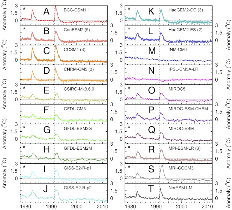
Of the 20 CMIP-5 models analyzed here, 18 models explicitly treat the radiative impact of aerosol particles injected into the stratosphere after major volcanic eruptions (Fig. 1). These aerosols absorb incoming solar radiation and outgoing long-wave radiation, leading to pronounced short-term (2–3 y) warming of the lower stratosphere (38). After the eruption of Pinatubo in 1991, the simulated maximum warming in TLS varies from roughly 1–3 °C. The two models that do not represent the full radiative effects of volcanic aerosols are IPSL-CM5A-LR and INM-CM4 (see Table S1 in SI Appendix for explanation of all model acronyms).

Fig. 1.

Time series of simulated monthly mean anomalies in TLS. Results are from spliced historical/RCP8.5 simulations performed with 20 individual CMIP-5 models (panels A–T). Anomalies were averaged over 82.5°N to 82.5°S, and are defined with respect to climatological monthly means from 1979 to 2011. The y axis range is identical in each panel. All available realizations of the spliced historical/RCP8.5 run are plotted; for models with more than one realization, the ensemble size is given in parentheses. For the CNRM-CM3 model, splicing was performed with the historicalExt simulation instead of RCP8.5 (SI Appendix). Dashed vertical lines indicate the start dates of the El Chichón and Pinatubo eruptions. Models used in estimating the O3+V fingerprint are identified with asterisks.

Human-caused depletion of stratospheric ozone is the main driver of lower stratospheric cooling over the satellite era (29, 38, 39). Of the 20 CMIP-5 models analyzed here, 7 are classified as CHEM models with fully interactive or semioffline calculation of ozone chemistry, and 13 as NOCHEM models with prescribed ozone changes (SI Appendix, Table S3).

Our fingerprint analysis involves a number of sensitivity tests (see below). In the first test, fingerprints were calculated using multimodel average temperature changes from 12 models with more reliable estimates of forcing by ozone and volcanic aerosols (O3+V; see Fig. 1). Because most CHEM models have errors in their simulations of historical ozone changes, the O3+V fingerprint was estimated with NOCHEM models only; 1 of the 13 NOCHEM models, INM-CM4, was excluded because of its incomplete treatment of volcanic aerosol forcing. We compare the 12-model O3+V results with the baseline (BASE) case, in which fingerprints were computed with model-average temperature changes from all 20 CMIP-5 models analyzed here (SI Appendix, Fig. S3).

The lower stratospheric cooling trend is nearly 10% larger in the more realistically forced O3+V subset than in the BASE subset, and it is closer to the observational results (SI Appendix, Table S7). Even in the O3+V case, however, the model-average cooling of the lower stratosphere from 1979 to 2011 is smaller than in all three observational TLS datasets, and smaller than in 9 of 11 RSS percentile realizations.

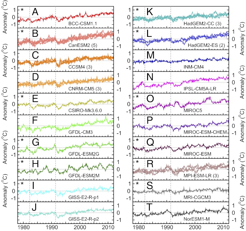
In the lower troposphere (Fig. 2), model TLT trends over the satellite era vary from 0.121 °C to 0.392 °C per decade (SI Appendix, Table S6). The BASE and O3+V multimodel average TLT trends are similar (0.262 °C and 0.266 °C per decade) and roughly 1.9 times larger than the RSS and UAH lower tropospheric temperature trends (0.139 °C and 0.140 °C per decade). There is no overlap between the 5–95 percentile ranges of the RSS trends and the multimodel average TLT trend results (SI Appendix, Table S7). Possible reasons for the biases in model TLS and TLT trends are discussed below.

Fig. 2.

The same as for Fig. 1, but for monthly mean anomalies in TLT. Results are from spliced historical/RCP8.5 simulations performed with 20 individual CMIP-5 models (panels A–T). Model anomalies are averaged over 82.5°N to 70°S.

Zonal Mean Temperature Trends

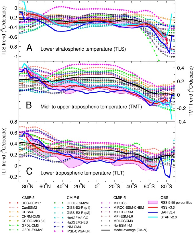
Fig. 3 shows zonal mean trends in TLS, TMT, and TLT from 1979 to 2011. All model results are for the O3+V case. For both lower stratospheric cooling and tropospheric warming, patterns of change at hemispheric scales are similar in models and observations. There are, however, some noticeable differences in the zonal mean structure of the modeled and observed temperature trends. Many of these differences are consistent across observational datasets, latitude, and altitude.

Fig. 3.

Zonal mean trends in observed and synthetic (A) TLS, (B) TMT, and (C) TLT between 1979 and 2011. Observational results are from UAH, STAR, version 3.3 of the RSS dataset, and the 11 RSS percentile realizations. Model synthetic MSU temperatures are from the spliced historical/RCP8.5 runs performed with 20 CMIP-5 models; only the first realization is shown for each model. The CMIP-5 multimodel averages are for the O3+V case. The 5th to 95th percentile range of the RSS results was computed as described in SI Appendix. The close agreement between RSS and UAH global mean TLT trends (SI Appendix, Table S7) masks large differences in the latitudinal structure of each group’s TLT changes. The spatial coverage of the observational datasets differs at high latitudes and over areas of high elevation (SI Appendix). Note that STAR does not produce a TLT dataset.

In the lower stratosphere, the O3+V model average cooling trend is smaller than in two of three observed datasets (UAH and STAR) over a wide range of latitudes (Fig. 3A). Poleward of roughly 60°N, the sign of the model TLS trend bias is reversed. In all tropospheric layers, the O3+V trends are biased warm over the Southern Hemisphere, tropics, and Northern Hemisphere midlatitudes, and are biased cool over the Arctic (Fig. 3 B and C and SI Appendix, Fig. S5). The multimodel average tropospheric temperature trends are outside the 5–95 percentile range of RSS results at most latitudes.

The likely causes of these biases include forcing errors in the historical simulations (40–42), model response errors (43), remaining errors in satellite temperature estimates (26, 44), and an unusual manifestation of internal variability in the observations (35, 45). These explanations are not mutually exclusive.

Our results suggest that forcing errors are a serious concern. Consider the example of stratospheric ozone forcing. At least three of seven CHEM models analyzed here (CCSM4, CNRM-CM5, and IPSL-CM5A-LR) appear to underestimate observed global mean ozone decreases over 1980–2000 by more than 50%. All three of these models underestimate the observed cooling of the lower stratosphere from 1979 to 2011 (compare SI Appendix, Table S6 with SI Appendix, Table S7).* This finding highlights the importance of accurate representation of stratospheric ozone changes for accurate simulation of TLS trends (3, 11, 39, 46–48).

Errors in ozone forcing are not restricted to CHEM models; many of the NOCHEM models may have also underestimated observed ozone loss over the satellite era (42). To date, it has been difficult to determine the contribution of ozone forcing errors to model biases in tropospheric temperature trends.^† Reliable quantification of this contribution is hampered by large uncertainties in observational estimates of ozone changes (42).

Based on analyses of earlier CMIP-3 results, a recent critique of fingerprint research claims that anthropogenic forcing by tropospheric aerosols could have been “tuned” to improve the correspondence between simulated and observed changes in global mean surface temperature (49). There are at least two reasons why such tuning concerns are unlikely to impact our S/N results: (i) fingerprint studies consider complex spatio-temporal patterns of climate change, and not global mean changes alone; and (ii) almost all modeling groups participating in CMIP-5 used the same prescribed aerosol precursor emissions.

Geographical Patterns of Temperature Trends

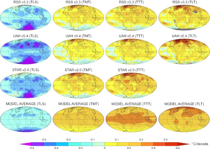
Fig. 4 shows geographical patterns of modeled (O3+V) and observed changes in atmospheric temperature from 1979 to 2011. Because some modeling groups produced ensembles of the spliced historical/RCP8.5 runs (SI Appendix, Table S4), temperature changes are first averaged over individual ensemble members and then averaged over the 12 O3+V models. The first averaging step reduces the noise introduced by internal variability, which can be large at high latitudes (SI Appendix, Fig. S4). The second averaging step reduces some of the smaller-scale pattern differences in the individual model responses to external forcing (SI Appendix, Figs. S6 and S7). This is why the simulated patterns of temperature change in Fig. 4 are noticeably smoother than the temperature changes in a single realization of the observations.

Fig. 4.

Geographical patterns of observed and simulated trends (in degrees Celsius per decade) in TLS, TMT, TTT, and TLT (columns 1–4, respectively). All trends are from 1979 to 2011. Simulated trends are the O3+V multimodel averages of synthetic MSU temperature changes from the spliced historical/RCP8.5 runs. Gray shading denotes areas where temperature information is not provided (SI Appendix).

In the lower stratosphere, there is a common signal of global-scale cooling in models and observations, with the largest cooling at high latitudes in the Southern Hemisphere. This cooling maximum is approximately zonally uniform in the O3+V multimodel average, but it is more wave-like in the observations. Satellite TLS trends exhibit secondary cooling maxima centered at roughly 40°N and 40°S (Fig. 3A). These cooling lobes are not evident in the multimodel average.

In the lower troposphere (Fig. 4), the O3+V models reproduce both the large-scale observed warming pattern from 1979 to 2011 and its hemispheric asymmetry. This asymmetry is characterized by maximum warming over the Arctic and minimum warming at high latitudes in the Southern Hemisphere. In the observations, hemispherically asymmetric warming of the lower troposphere is physically consistent with ice/albedo feedbacks arising from the large decrease in Arctic sea ice extent and the smaller increase in Antarctic sea ice coverage (50, 51).

The muted lower tropospheric warming over the Antarctic has not been fully explained. There is considerable evidence that the large human-caused decline in stratospheric ozone over this region is the primary driver of recent multidecadal changes in the intensity of the Southern Hemisphere polar vortex (52, 53). Such externally forced circulation changes can affect Antarctic sea ice extent (51, 54), although the strength (and even the direction) of this effect is still unclear (55). Model simulations with combined forcing by well-mixed greenhouse gases and stratospheric ozone are capable of replicating observed changes in the intensity of the Antarctic polar vortex (52, 53), implying that some of the factors driving hemispheric-scale asymmetries in patterns of tropospheric trends may be similar in models and observations.

In the mid to upper troposphere and total troposphere, models and observations also show a common pattern of hemispherically asymmetric warming (Fig. 4). The O3+V warming pattern, however, is larger and more coherent than in observations, and it does not reproduce the Arctic warming maximum evident in satellite TMT and TTT datasets. The enhanced tropical warming in the simulated TTT results is due to both the pronounced warm bias in the O3+V tropical TMT trends and the smaller than observed tropical TLS trends.

Evaluating Model Noise Estimates

Model estimates of internal climate variability are a key component of detection and attribution (D&A) studies (5, 35). Here, we describe how we selected subsets of models with more credible estimates of the size of atmospheric temperature variability. We also address the question of whether CMIP-5 models systematically underestimate observed temperature variability, which would spuriously inflate the S/N ratios in our D&A analysis.

One strategy in model vs. observed variability comparisons is to estimate and remove externally forced climate signals from the observations, and then compare the residual variability with control run internal variability (4). There are a number of uncertainties in such signal removal strategies (17). We use a different approach here, and directly compare estimates of the total variability (arising from both natural external forcing and processes internal to the climate system) in the observations and the spliced historical/RCP8.5 runs.

Our analysis period extends from January 1979 to December 2011. After detrending modeled and observed time series of globally averaged monthly mean temperature anomalies, we applied a band-pass filter with half-power points at 5 and 20 y to the residuals (35). We also used a high-pass filter to extract variability information on 1- to 2-y timescales (SI Appendix).

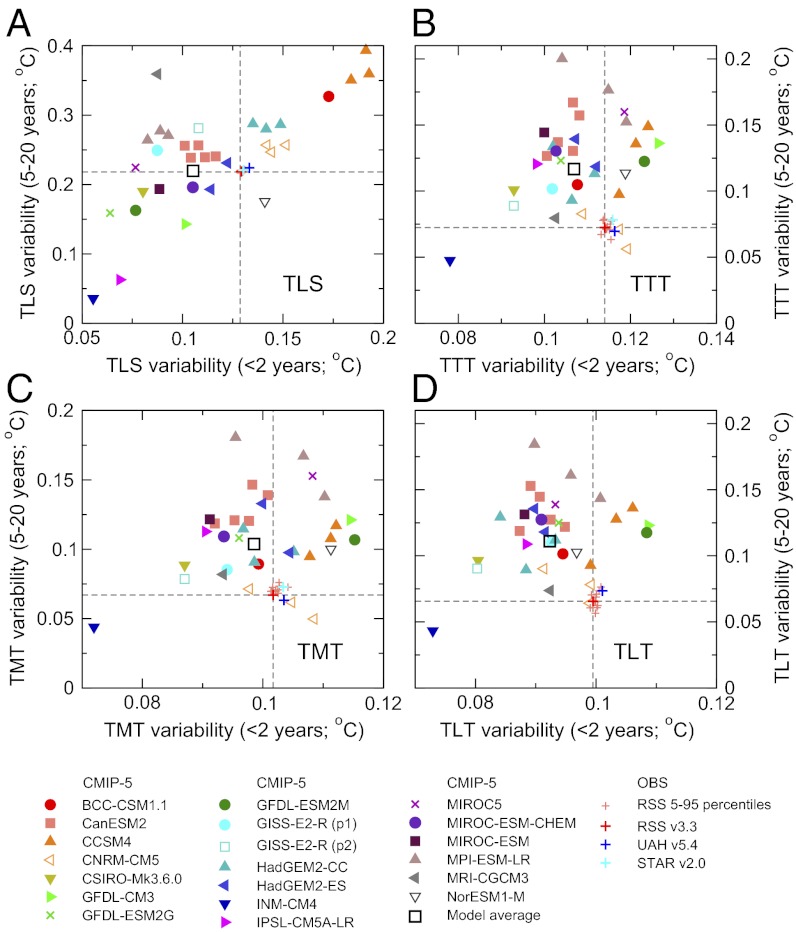
Because the decadal variability is more important in D&A applications, only band pass-filtered results were used in ranking and selecting the five models closest to observations (TOP-5). Model ranking was based on , the temporal standard deviation of the band-pass-filtered data, and it relied on RSS v3.3 results as the observational target. Model vs. observed differences in are much larger than the observational uncertainties in this metric, so the choice of observational target has little influence on the ranking results.

For TLS, the model average and observed values are almost identical (Fig. 5A). In the troposphere, the multimodel average value of is 55–69% larger than the RSS values (Fig. 5 B–D). On 5- to 20-y timescales, therefore, we find no evidence that CMIP-5 models systematically underestimate the amplitude of observed atmospheric temperature variability. In contrast, the CMIP-5 models underestimate variability on 1- to 2-y timescales by an average of 3–7% in the troposphere and 19% in the stratosphere. This finding may be partly because of differences in how atmospheric temperature is sampled in models and observations.^‡

Fig. 5.

Comparison of simulated and observed variability of monthly mean near-global anomalies in (A) TLS, (B) TTT, (C) TMT, and (D) TLT. In each panel, the monthly to interannual timescale variability of detrended, high pass-filtered temperature data (, x axis) is plotted against the 5- to 20-y timescale variability of band pass-filtered data (, y axis). The dashed lines are centered on the observed values of and for version 3.3 of the RSS dataset. The multimodel average and values were calculated by averaging over the ensemble mean and results for each of the 20 individual CMIP-5 models. The same 396 months (January 1979 to December 2011) were used for the analysis of observations and synthetic MSU temperatures from the spliced historical/RCP8.5 runs.

Fingerprint Method

Detection and attribution studies require an estimate of the climate signal in response to external forcing. This signal is the fingerprint. Fingerprints are defined in a number of different ways (19). Typically, they provide information about the signal’s spatial properties or combined space–time structure. This information is valuable in discriminating between two external forcings with similar global mean signals, but with different patterns or timescales of climate response (1, 2).

In most applications, the climate change fingerprint is a geographical pattern (4, 12), a vertical profile through the atmosphere or ocean (3, 9, 11), or a vector with information on the combined spatial and temporal properties of the signal (6–8). Here, the fingerprint is a fixed geographical pattern, calculated with the time-varying atmospheric temperature changes from 1861 to 2011 in the CMIP-5 historical/RCP8.5 simulations (SI Appendix). provides an estimate of the century-timescale climate response to external forcing by a combination of human and natural factors.

The implicit assumption in this approach is that the spatial pattern of response does not change markedly over time (56). This assumption is unlikely to hold, particularly for externally forced changes in lower stratospheric temperature. We examine the impact of this assumption on S/N results by defining the fingerprint over different time intervals. Even in the case of TLS changes, the nonstationarity of does not hamper fingerprint detection in the observations (SI Appendix).

In the next section, we focus on S/N ratios obtained with the O3+V fingerprint (calculated over 1861 to 2011) and internal variability information from the TOP-5 models. SI Appendix provides S/N results from a number of additional sensitivity tests, which consider the choice of an alternative period for calculating (1979–2011), as well as the use of alternative fingerprint and noise estimates (obtained from the BASE models).

Fingerprint Results

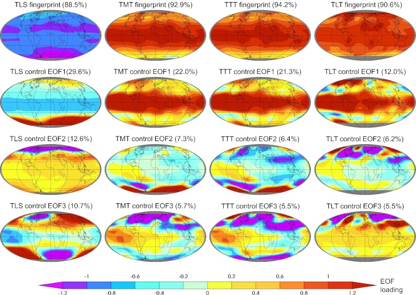
The O3+V fingerprints (Fig. 6, row 1) have temperature changes of the same sign at virtually all grid points, and primarily reflect the global-scale cooling of the lower stratosphere and warming of the troposphere. The fingerprints preserve the above-described hemispheric differences in temperature change signals, such as the enhanced warming of the Arctic relative to the Antarctic in the lower troposphere. In contrast, the three leading noise modes estimated from the TOP-5 control runs do not have the same spatial coherence of temperature changes; they are characterized by variability at smaller spatial scales (Fig. 6, rows 2–4).

Fig. 6.

Leading signal and noise modes from the pattern-based S/N analysis, together with the percentage variance explained by each mode. Results are for TLS, TMT, TTT, and TLT (columns 1–4, respectively). The fingerprint is the leading empirical orthogonal function (EOF) of multimodel average atmospheric temperature changes between 1861 and 2011. Fingerprints were calculated with synthetic MSU temperatures from the spliced historical/RCP8.5 runs, using results from the 12 O3+V models (row 1). The leading noise modes are EOFs 1, 2, and 3 of the concatenated preindustrial control runs (rows 2–4, respectively). Only the TOP-5 CMIP-5 models were used in noise estimation. Details of fingerprint and noise mode calculations are in SI Appendix.

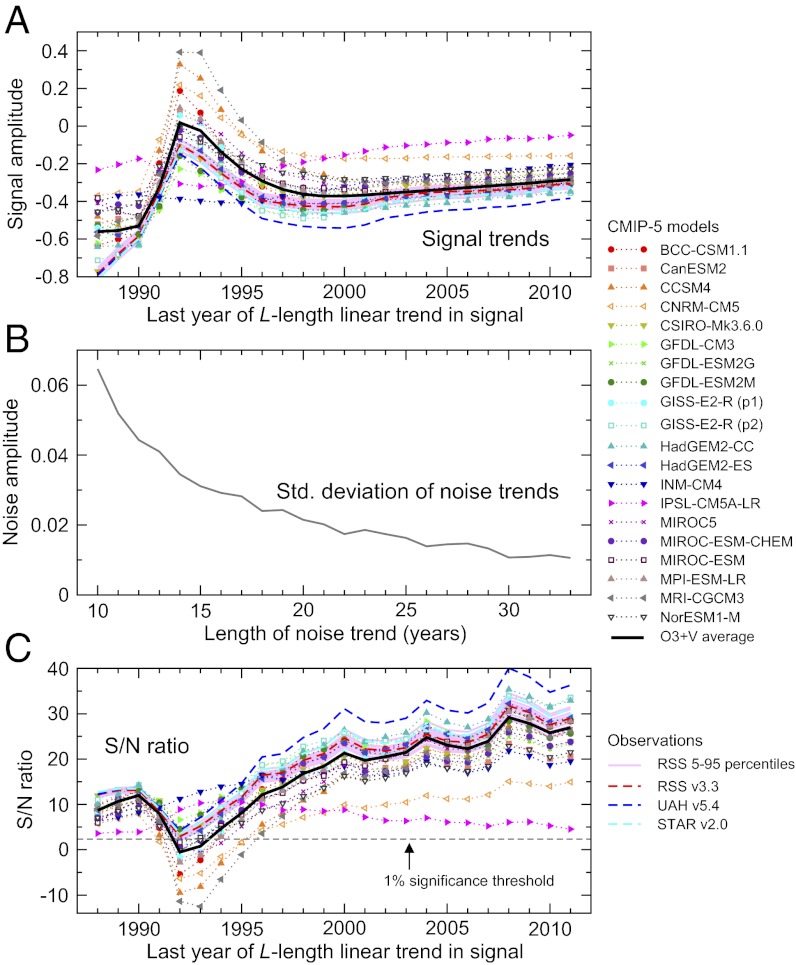
In our D&A analysis, atmospheric temperature changes from observations and the historical/RCP8.5 simulations are projected onto , yielding signal time series. We fit trends of increasing length L to these time series. TLS signal trends are shown in Fig. 7A. As L increases, the Pinatubo-induced stratospheric warming in 1992 and 1993 damps stratospheric cooling trends, except in the two models without absorption of solar and outgoing long-wave radiation by volcanic aerosols (INM-CM4 and IPSL-CM5A-LR). After recovery from Pinatubo, stratospheric cooling trends show relatively little change as the trend-fitting period increases.

Fig. 7.

Results from the D&A analysis of simulated and observed changes in lower stratospheric temperature. Signal time series provide information on the similarity between the time-invariant TLS fingerprint pattern and the time-varying patterns of lower stratospheric temperature change in observations and individual model simulations of forced climate change. The L year trends in these signal time series are plotted in A. The noise time series indicate the level of similarity between the fingerprint and the TOP-5 model estimates of internal variability. The standard deviation of the distribution of L year trends in the noise time series, , is plotted in B. The S/N ratio between L year signal trends (A) and values of (B) is shown in C. The TLS fingerprint is for the O3+V case, calculated using the multimodel average TLS changes from 1861 to 2011 (Fig. 6). The model average results in A and C are the projections of the O3+V multimodel average TLS changes onto the O3+V fingerprint. The sign of signal trends is stipulated to be negative in A (because models and observations both show cooling of the lower stratosphere), and the absolute value of the S/N ratio is plotted in C. Full details of the D&A analysis are in SI Appendix.

Our noise time series are obtained by projecting temperature changes from the concatenated control runs onto . As in the case of the signals, we fit L year trends to the noise time series. The noise trends decrease in amplitude as the trend-fitting period increases (Fig. 7B), which is a well-known property of many meteorological and oceanographic time series (35). The decay in the size of noise trends is the primary driver of the increase in S/N ratios with longer trend-fitting periods (Fig. 7C).

We discuss two different types of S/N ratio. The first type provides information on the strength of the fingerprint in observational temperature data (relative to fingerprint strength in model internal variability estimates). The second type of S/N ratio involves no observational data, and quantifies the strength of in each individual model’s forced atmospheric temperature changes. We refer to these subsequently as model-observed and model–model S/N ratios.

For TLS signal trends from 1979 to 2011, model-observed S/N ratios range from 26 to 36, depending on the observational dataset used (a S/N ratio greater than 2.33 is significant at the 1% level). These results indicate that natural internal variability is highly unlikely to explain the time-increasing similarity between the O3+V fingerprint and observed patterns of lower stratospheric temperature change. The large range of model–model S/N ratios (from 4 to 29) primarily reflects intermodel differences in the size of the lower stratospheric cooling signal (SI Appendix, Table S6).

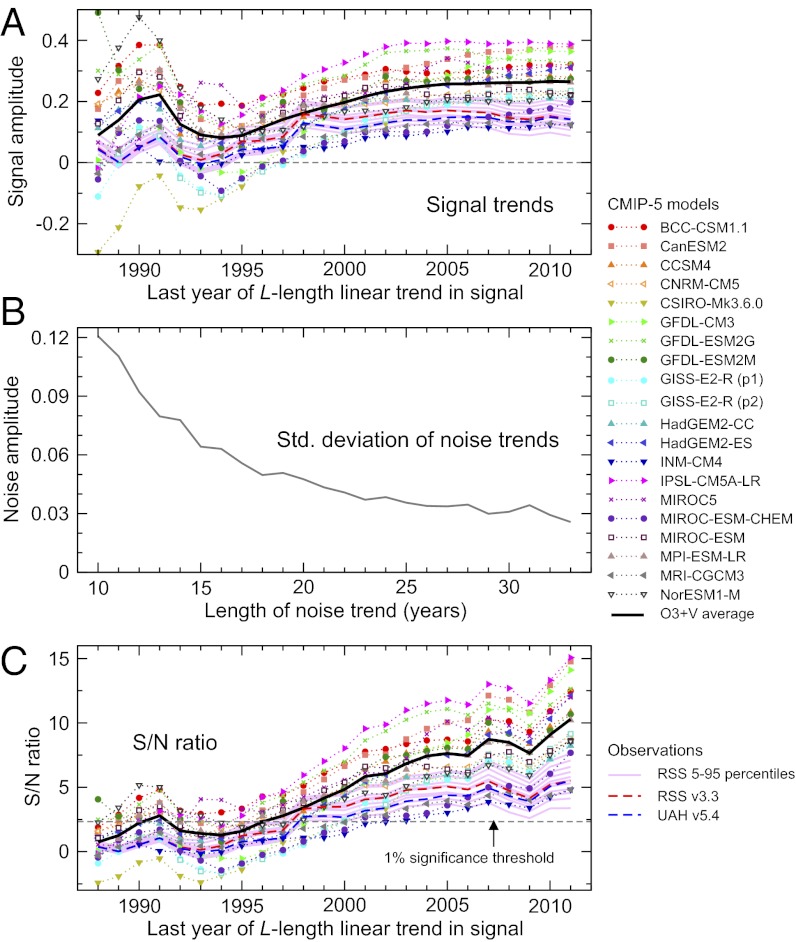
In the lower troposphere, signal trends in most individual models and observational datasets increase as the trend length L increases, but trends show little change after 2005 (Fig. 8A). The decline in the size of TLT signal trends in the early 1990s is caused by the cooling effect of Pinatubo on tropospheric temperature. As for TLS, the decrease in the size of noise trends with increasing trend length is the main cause of the overall increase in S/N ratios (Figs. 8 B and C).

Fig. 8.

The same as in Fig. 7, but for changes in TLT. Results are for signal trends (A), noise trends (B), and S/N ratios (C).

Model-observed S/N ratios for 33-y TLT signal trends are smaller than in the TLS case, but still highly significant (Fig. 8C). The RSS 5th and 95th percentiles yield the lowest and highest S/N ratios (3.4 and 7.6). Model–model S/N ratios vary from 4.8 to 15.1 for 33-y TLT trends, and scale with intermodel differences in global mean tropospheric warming (SI Appendix, Table S6). Only the INM-CM4 and MRI-CGCM3 models have 33-y model–model S/N ratios contained within the RSS 5th to 95th percentile range.

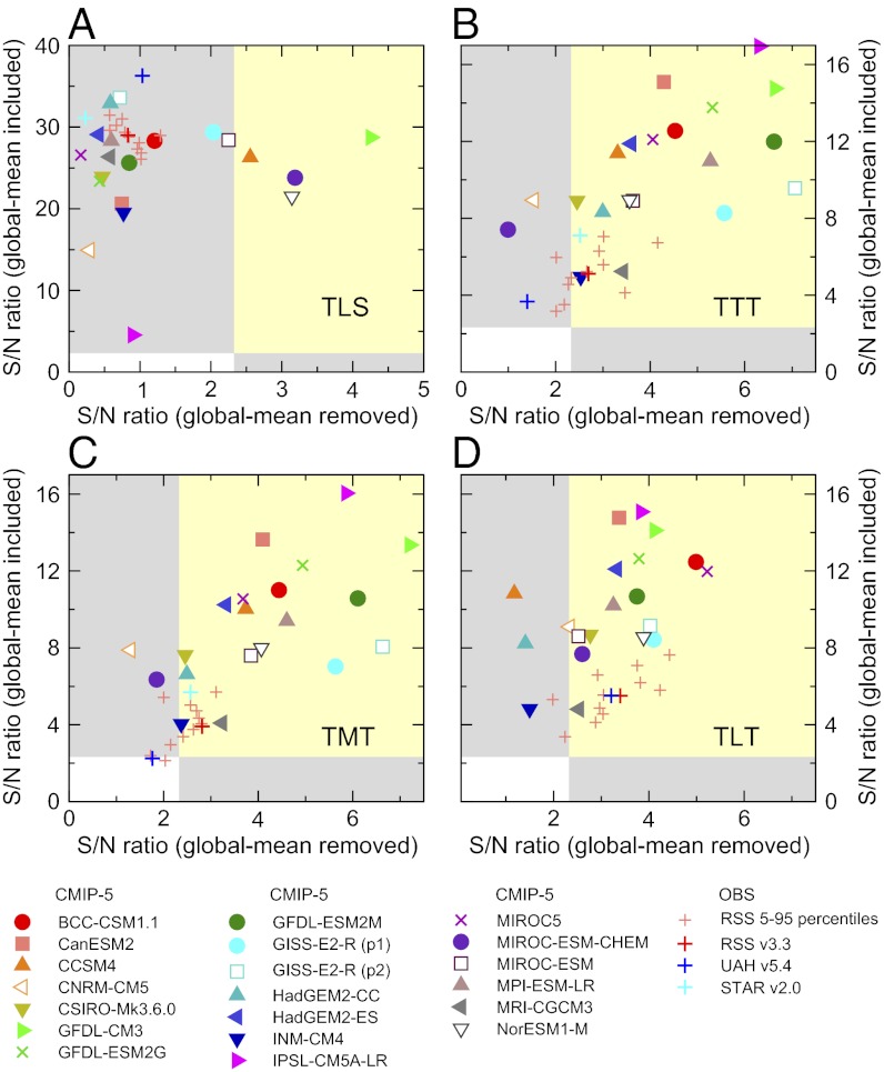
Fig. 9 summarizes these results, and shows S/N ratios for trends over the full 33-y satellite era. Results are for each of the four atmospheric temperature variables, and for cases with and without the global mean component of temperature change. In the latter, global mean temperature changes in each year of each model and observational dataset were removed before calculation of S/N ratios, so that large S/N ratios can only reflect true pattern similarity.

Fig. 9.

Summary plot of S/N ratios for (A) TLS, (B) TTT, (C) TMT, and (D) TLT. Results are for trends over the entire 33-y satellite record (1979–2011). The D&A analysis was performed in two different ways: with removal of the global mean component of temperature change from each model and observational dataset, and with the global mean change included. Results for these two processing choices are plotted on the x and y axes, respectively. The S/N analysis relies on the O3+V fingerprints (estimated using multimodel average temperature changes from 1861 to 2011) and the TOP-5 model noise estimates. The yellow shading denotes the region where S/N ratios are significant at the 1% level or better for both the global mean removed and global mean included cases. In the gray shaded regions, statistically significant S/N ratios are obtained in only one of these two cases. See Figs. 7 and 8 and SI Appendix for additional information.

Consider first the results with the global mean included. For model-observed S/N ratios, there are a total of 55 comparisons.^§ In 53 of these comparisons, S/N ratios are significant at the 1% level, and the model-predicted O3+V fingerprint is identifiable with high statistical confidence in the observed datasets.

When information on global mean temperature changes is removed, the O3+V fingerprint is still detectable in over 50% of the model-observed comparisons (29 of 55 cases). In the lower troposphere, the global mean removed fingerprint is identifiable in 11 of 13 observational TLT datasets (Fig. 9D), because the pronounced warming of the Arctic relative to the Antarctic is common to the fingerprint and the observations. The global mean removed fingerprint is also identifiable in 9 observational TTT records and 9 observational TMT datasets (Fig. 9 B and C).

In the lower stratosphere, however, the global mean removed fingerprint is not detectable in any of the 14 observational TLS datasets (Fig. 9A). This null result occurs because the O3+V fingerprint does not capture the full subglobal structure of observed TLS trends, particularly the lobes of pronounced cooling at 40°N and 40°S (Figs. 3A and 4).

Conclusions

We used a multimodel archive to obtain fingerprints of atmospheric temperature change. These fingerprints are estimates of the climate responses to external forcing by the combined effects of anthropogenic factors, volcanoes, and solar irradiance. The primary components of external forcing over the past century are human-caused increases in well-mixed greenhouse gases, depletion of stratospheric ozone, and changes in atmospheric burdens of various aerosol particles (20, 57). Our fingerprints, therefore, mainly reflect human influences on climate (7, 19, 29).

When global mean changes were included in our detection method, we were able to identify the model fingerprints with high statistical confidence in 53 of 55 model data comparisons. For changes in TLS from 1979 to 2011, S/N ratios varied from 26 to 36, depending on the choice of observational dataset. For changes in TLT, S/N ratios ranged from roughly three to eight. Although the TLT ratios are lower than for TLS, they are still highly significant.

There is no evidence that these results are spuriously inflated by model variability errors. In the troposphere, CMIP-5 estimates of variability on 5- to 20-y timescales are (on average) 55–69% larger than in observations. In the lower stratosphere, observed and model average estimates of 5- to 20-y variability are of similar size. This finding suggests that our S/N ratios for multidecadal trends are conservative, and that our inferences regarding fingerprint detection are also likely to be conservative.

We repeated our S/N analysis after removing global mean temperature change information from all datasets. This analysis provides a more stringent test of the ability of models to represent observed temperature change patterns. In the lower troposphere, the global mean removed fingerprint was detected in 11 of 13 observational datasets. Positive detection arises because of a common signal of warming of the Arctic relative to the Antarctic. For lower stratospheric temperature changes, however, the subglobal features of the model TLS fingerprint were not detectable in any observational dataset.

Our fingerprint results are interpretable in terms of basic physical mechanisms. The global-scale lower stratospheric cooling is primarily a direct radiative response to human-caused depletion of stratospheric ozone (29, 39, 58). Tropospheric warming is mainly driven by human-caused increases in well-mixed greenhouse gases (16, 29). The multidecadal cooling of the stratosphere and warming of the troposphere, which is evident in all satellite datasets and simulations of forced climate change examined here, cannot be explained by solar or volcanic forcing, or by any known mode of internal variability (3, 11).

Our ability to identify an externally forced fingerprint in satellite estimates of atmospheric temperature change is robust to current uncertainties in both models and observations, and to choices made in the application of our fingerprint method (SI Appendix). However, important questions still remain. Although we found a match between modeled and observed geographical patterns of temperature change, there are still noticeable differences in the size of these changes. On average, the CMIP-5 models underestimate the observed cooling of the lower stratosphere and overestimate the warming of the troposphere. Biases are largest over the tropics and the Southern Hemisphere. Results presented here and elsewhere (40–42) suggest that forcing errors make an important contribution to such biases. These results point to the need for a more systematic exploration of the impact of forcing uncertainties on simulations of historical climate change.

References

- 1.Hasselmann K. On the signal-to-noise problem in atmospheric response studies. In: Shaw DB, editor. Meteorology of Tropical Oceans. London: Royal Meteorology Society; 1979. pp. 251–259. [Google Scholar]
- 2.North GR, Kim KY, Shen SSP, Hardin JW. Detection of forced climate signals. Part 1: Filter theory. J Clim. 1995;8:401–408. [Google Scholar]
- 3.Santer BD, et al. A search for human influences on the thermal structure of the atmosphere. Nature. 1996;382:39–46. [Google Scholar]
- 4.Hegerl GC, et al. Detecting greenhouse-gas-induced climate change with an optimal fingerprint method. J Clim. 1996;9:2281–2306. [Google Scholar]
- 5.Allen MR, Tett SFB. Checking for model consistency in optimal fingerprinting. Clim Dyn. 1999;15:419–434. [Google Scholar]
- 6.Stott PA, et al. External control of 20th century temperature by natural and anthropogenic forcings. Science. 2000;290(5499):2133–2137. doi: 10.1126/science.290.5499.2133. [DOI] [PubMed] [Google Scholar]
- 7.Tett SFB, et al. Estimation of natural and anthropogenic contributions to twentieth century temperature change. J Geophys Res. 2002 doi: 10.1029/2000JD000028. [DOI] [Google Scholar]
- 8.Gillett NP, et al. Detecting anthropogenic influence with a multi-model ensemble. Geophys Res Lett. 2002;29:1970. [Google Scholar]
- 9.Barnett TP, et al. Penetration of human-induced warming into the world’s oceans. Science. 2005;309(5732):284–287. doi: 10.1126/science.1112418. [DOI] [PubMed] [Google Scholar]
- 10.Karoly DJ, et al. An example of fingerprint detection of greenhouse climate change. Clim Dyn. 1994;10:97–105. [Google Scholar]
- 11.Tett SFB, Mitchell JFB, Parker DE, Allen MR. Human influence on the atmospheric vertical temperature structure: Detection and observations. Science. 1996;274(5290):1170–1173. doi: 10.1126/science.274.5290.1170. [DOI] [PubMed] [Google Scholar]
- 12.Santer BD, et al. Influence of satellite data uncertainties on the detection of externally forced climate change. Science. 2003a;300(5623):1280–1284. doi: 10.1126/science.1082393. [DOI] [PubMed] [Google Scholar]
- 13.Thorne PW, et al. Assessing the robustness of zonal mean climate change detection. Geophys Res Lett. 2002 doi: 10.1029/2002GL015717. [DOI] [Google Scholar]
- 14.Sexton DMH, Rowell DP, Folland CK, Karoly DJ. Detection of anthropogenic climate change using an atmospheric GCM. Clim Dyn. 2001;17:669–685. [Google Scholar]
- 15.Jones GS, Tett SFB, Stott PA. Causes of atmospheric temperature change 1960-2000: A combined attribution analysis. Geophys Res Lett. 2003 doi: 10.1029/2002GL016377. [DOI] [Google Scholar]
- 16.Hansen JE, et al. Efficacy of climate forcings. J Geophys Res. 2005 doi: 10.1029/2005JD005776. [DOI] [Google Scholar]
- 17. Santer BD, Wigley TML, Barnett TP, Anyamba E (1996) Detection of climate change and attribution of causes. Climate Change 1995: The Science of Climate Change, Contribution of Working Group I to the Second Assessment Report of the Intergovernmental Panel on Climate Change, eds Houghton JT, et al. (Cambridge Univ Press, Cambridge, UK)
- 18.Karl TR, Hassol SJ, Miller CD, Murray WL, editors. Temperature Trends in the Lower Atmosphere: Steps for Understanding and Reconciling Differences. A Report by the U.S. Climate Change Science Program and the Subcommittee on Global Change Research. Asheville, NC: National Oceanic and Atmospheric Administration, National Climatic Data Center; 2006. [Google Scholar]
- 19. Hegerl GC, et al. (2007) Understanding and attributing climate change. Climate Change 2007: The Physical Science Basis, Contribution of Working Group I to the Fourth Assessment Report of the Intergovernmental Panel on Climate Change, eds Solomon S, et al. (Cambridge Univ Press, Cambridge, UK)
- 20. Forster P, et al. (2007) Changes in atmospheric constitutents and in radiative forcing. Climate Change 2007: The Physical Science Basis, Contribution of Working Group I to the Fourth Assessment Report of the Intergovernmental Panel on Climate Change, eds Solomon S, et al. (Cambridge Univ Press, Cambridge, UK)
- 21.Thorne PW, Lanzante JR, Peterson TC, Seidel DJ, Shine KP. Tropospheric temperature trends: History of an ongoing controversy. Wiley Interdisciplinary Reviews. 2011;2:66–88. [Google Scholar]
- 22.Seidel DJ, Gillett NP, Lanzante JR, Shine KP, Thorne PW. Stratospheric temperature trends: Our evolving understanding. Wiley Interdisciplinary Reviews. 2011;2:592–616. [Google Scholar]
- 23.Wentz FJ, Schabel M. Effects of orbital decay on satellite-derived lower-tropospheric temperature trends. Nature. 1998;394:661–664. [Google Scholar]
- 24.Mears CA, Schabel MC, Wentz FW. A reanalysis of the MSU channel 2 tropospheric temperature record. J Clim. 2003;16:3650–3664. [Google Scholar]
- 25.Mears CA, Wentz FJ. The effect of diurnal correction on satellite-derived lower tropospheric temperature. Science. 2005;309(5740):1548–1551. doi: 10.1126/science.1114772. [DOI] [PubMed] [Google Scholar]
- 26.Mears C, Wentz FJ, Thorne P, Bernie D. Assessing uncertainty in estimates of atmospheric temperature changes from MSU and AMSU using a Monte-Carlo technique. J Geophys Res. 2011 doi: 10.1029/2010JD014954. [DOI] [Google Scholar]
- 27.Christy JR, Norris WB, Spencer RW, Hnilo JJ. Tropospheric temperature change since 1979 from tropical radiosonde and satellite measurements. J Geophys Res. 2007 doi: 10.1029/2005JD006881. [DOI] [Google Scholar]
- 28.Zou CZ, et al. Recalibration of microwave sounding unit for climate studies using simultaneous nadir overpasses. J Geophys Res. 2006 doi: 10.1029/2005JD006798. [DOI] [Google Scholar]
- 29.Santer BD, et al. Contributions of anthropogenic and natural forcing to recent tropopause height changes. Science. 2003b;301(5632):479–483. doi: 10.1126/science.1084123. [DOI] [PubMed] [Google Scholar]
- 30.Bonfils C, et al. Detection and attribution of temperature changes in the mountainous western United States. J Clim. 2008;21:6404–6424. [Google Scholar]
- 31.Santer BD, et al. Incorporating model quality information in climate change detection and attribution studies. Proc Natl Acad Sci USA. 2009;106(35):14778–14783. doi: 10.1073/pnas.0901736106. [DOI] [PMC free article] [PubMed] [Google Scholar]
- 32.Gleckler PJ, et al. Human-induced global ocean warming on multi-decadal time scales. Nat Clim Change. 2012;2:524–529. [Google Scholar]
- 33.Taylor KE, Stouffer RJ, Meehl GA. An overview of CMIP5 and the experiment design. Bull Am Meteor Soc. 2012;93(4):485–498. [Google Scholar]
- 34.Meinshausen M, et al. The RCP greenhouse gas concentrations and their extensions from 1765 to 2300. Clim Change. 2011;109(1–2):213–241. [Google Scholar]
- 35.Santer BD, et al. Separating signal and noise in atmospheric temperature changes: The importance of timescale. J Geophys Res. 2011 doi: 10.1029/2011JD016263. [DOI] [Google Scholar]
- 36.Fu Q, Johanson CM, Warren SG, Seidel DJ. Contribution of stratospheric cooling to satellite-inferred tropospheric temperature trends. Nature. 2004;429(6987):55–58. doi: 10.1038/nature02524. [DOI] [PubMed] [Google Scholar]
- 37.Fu Q, Johanson CM. Satellite-derived vertical dependence of tropical temperature trends. Geophys Res Lett. 2005 doi: 10.1029/2004GL22266. [DOI] [Google Scholar]
- 38.Ramaswamy V, et al. Stratospheric temperature trends: Observations and model simulations. Rev Geophys. 2001;39:71–122. [Google Scholar]
- 39.Ramaswamy V, et al. Anthropogenic and natural influences in the evolution of lower stratospheric cooling. Science. 2006;311(5764):1138–1141. doi: 10.1126/science.1122587. [DOI] [PubMed] [Google Scholar]
- 40.Solomon S, et al. Contributions of stratospheric water vapor to decadal changes in the rate of global warming. Science. 2010;327(5970):1219–1223. doi: 10.1126/science.1182488. [DOI] [PubMed] [Google Scholar]
- 41.Solomon S, et al. The persistently variable “background” stratospheric aerosol layer and global climate change. Science. 2011;333(6044):866–870. doi: 10.1126/science.1206027. [DOI] [PubMed] [Google Scholar]
- 42.Solomon S, Young PJ, Hassler B. Uncertainties in the evolution of stratospheric ozone and implications for recent temperature changes in the tropical lower stratosphere. Geophys Res Lett. 2012 doi: 10.1029/2012GL052723. [DOI] [Google Scholar]
- 43.Trenberth KE, Fasullo JT. Simulation of present-day and twenty-first-century energy budgets of the Southern Oceans. J Clim. 2010 doi: 10.1175/2009JCL3152.1. [DOI] [Google Scholar]
- 44.Po-Chedley S, Fu Q. A bias in the mid-tropospheric channel warm target factor on the NOAA-9 microwave sounding unit. J Atmos Ocean Technol. 2012;29:646–652. [Google Scholar]
- 45.Fu Q, Manabe S, Johanson CM. On the warming in the tropical upper troposphere: Models versus observations. Geophys Res Lett. 2011 doi: 10.1029/2011GL048101. [DOI] [Google Scholar]
- 46.Lanzante JR. Diagnosis of radiosonde vertical temperature trend profiles: Comparing the influence of data homogenization versus model forcings. J Clim. 2007;20:5356–5364. [Google Scholar]
- 47.Hu Y, Xia Y, Fu Q. Tropospheric temperature response to stratospheric ozone recovery in the 21st century. Atmos Chem Phys. 2011;11:7687–7699. [Google Scholar]
- 48.McLandress C, Perlwitz J, Shepherd TG. Comment on “Tropospheric temperature response to stratospheric ozone recovery in the 21st century” by Hu et al. (2011) Atmos Chem Phys. 2012;12:2533–2540. [Google Scholar]
- 49.Curry JA, Webster PJ. Climate science and the uncertainty monster. Bull Am Meteor Soc. 2011;92(12):1667–1682. [Google Scholar]
- 50.Stroeve J, Holland MM, Meier W, Scambos T, Serreze MC. Arctic sea ice decline: Faster than forecast. Geophys Res Lett. 2007;34:L09501. [Google Scholar]
- 51.Turner J, et al. Non-annular atmospheric circulation change induced by stratospheric ozone depletion and its role in the recent increase of Antarctic sea ice extent. Geophys Res Lett. 2009;36:L08502. [Google Scholar]
- 52.Arblaster JM, Meehl GA. Contributions of external forcings to Southern Annular Mode trends. J Clim. 2006;19:2896–2905. [Google Scholar]
- 53.Karpechko AY, Gillett NP, Marshall GJ, Scaife AA. Stratospheric influence on circulation changes in the Southern Hemisphere troposphere in coupled climate models. Geophys Res Lett. 2008;35:L20806. [Google Scholar]
- 54.Goosse H, Lefebvre W, Montety A, Crespin E, Orsi AH. Consistent past half-century trends in the atmosphere, the sea ice and the ocean at high southern latitudes. Clim Dyn. 2009;33:999–1016. [Google Scholar]
- 55.Sigmond M, Fyfe JC. Has the ozone hole contributed to increased Antarctic sea ice extent? Geophys Res Lett. 2010;37:L18502. [Google Scholar]
- 56.Wigley TML, Jaumann PJ, Santer BD, Taylor KE. Relative detectability of greenhouse-gas and aerosol climate change signals. Clim Dyn. 1998;14:781–790. [Google Scholar]
- 57.Wigley TML, Santer BD. A probabilistic quantification of the anthropogenic component of 20th century global warming. Clim Dyn. 2012 doi: 10.1007/s00382-012-1585-8. [DOI] [Google Scholar]
- 58.Gillett NP, et al. Attribution of observed changes in stratospheric ozone and temperature. Atmos Chem Phys. 2011;11:599–609. [Google Scholar]
Associated Data
This section collects any data citations, data availability statements, or supplementary materials included in this article.