Obscuring Surface Anatomy in Volumetric Imaging Data

Abstract

The identifying or sensitive anatomical features in MR and CT images used in research raise patient privacy concerns when such data are shared. In order to protect human subject privacy, we developed a method of anatomical surface modification and investigated the effects of such modification on image statistics and common neuroimaging processing tools. Common approaches to obscuring facial features typically remove large portions of the voxels. The approach described here focuses on blurring the anatomical surface instead, to avoid impinging on areas of interest and hard edges that can confuse processing tools. The algorithm proceeds by extracting a thin boundary layer containing surface anatomy from a region of interest. This layer is then “stretched” and “flattened” to fit into a thin “box” volume. After smoothing along a plane roughly parallel to anatomy surface, this volume is transformed back onto the boundary layer of the original data. The above method, named normalized anterior filtering, was coded in MATLAB and applied on a number of high resolution MR and CT scans. To test its effect on automated tools, we compared the output of selected common skull stripping and MR gain field correction methods used on unmodified and obscured data. With this paper, we hope to improve the understanding of the effect of surface deformation approaches on the quality of de-identified data and to provide a useful de-identification tool for MR and CT acquisitions.

Introduction

Imaging methods, such as MRI and CT, are now commonly used in biomedical research. MR and CT images of the head may be used to create high resolution representations of the face, potentially allowing to identify the human subjects involved in such research. Several studies (Prior et al. 2009; Chen et al. 2007; Budin et al. 2008) examined the ability of human observers to identify a facial anatomy rendering with an image as presented in a photograph set. Budin et al. (2008) indicated that the chance of correctly connecting a 3D face rendering with a photographic portrait is higher than random guess, and Prior et al. (2009) also reported statistical significance of such probability. On the other hand, named studies report high difficulty of recognition experienced by raters, which may indicate that, while maintaining a potential privacy risk, facial anatomy renderings are still very poor substitutes for a photograph.

Although recognition by human observer may be difficult, progress in automatic face recognition software may also increase the risk of identification. Mazura et al. (2011) explored the ability of automatic face recognition software to identify 3D face renderings of CT scans, reporting the success in identification of 27.5 % of 3D renderings with photographs. Ability to automatically analyze face renderings on high volumes of 3D data may increase the probability of occasional identification.

With the increasingly common practice of sharing imaging data within the research community, including via open access resources (Marcus et al. 2007a), the need for methods to protect the privacy of the human subjects is of great importance. Within the United States, the requirements for patient and research subject privacy are described in the HIPAA¹; in particular, identifying information that should be removed includes photographs and equivalent images. Several techniques have been developed to remove potentially identifiable features from images, especially to prevent face recognition.

Many prior de-identification methods have employed pre-existing techniques that were developed for other purposes, such as MR skull stripping, a common preprocessing step in many neuroimaging studies. Skull stripping algorithms such as (Smith 2002) classify voxels into brain and non-brain, and leave only brain voxels in the dataset. This approach has the drawback that it removes anatomical features that are necessary to calculate important values such as intracranial volume and cerebrospinal fluid volume. A variation on this approach used to de-identify the open access dataset (Marcus et al. 2007a) involved creating brain mask using skull stripping and then enlarging this mask slightly. This approach has the advantage that it preserves the cranial vault. In our experience, however, skull stripping requires careful supervision and may be affected by variation in diagnoses, age groups, MR field inhomogeneity, etc. (Fennema-Notestine et al. 2006).

Since skull stripping methods remove too much data, some investigators employed voxel masking methods that remove only part of surface voxels pertaining to face only. For example, an approach implemented by Bischoff-Grethe et al. (2007) suggests removing only corresponding skull structures. Their method uses an atlas registration framework together with Bayesian classifier for generating facial anatomy probability map. The algorithm further removes voxels that have high probability of belonging to orbits, nasal cavity, or lower/upper jaws. The authors ran several different brain extraction algorithms on de-identified data; their evidence suggests that their face stripping preprocessing step has little effect on the outcome of skull stripping.

De-identification methods based on segmentation of tissues or external organs require a voxel classifier, which usually works best when tuned to specific data characteristics such as specific body part, contrast mechanism and other acquisition parameters, or demographic and pathology characteristics of a training sample. Using a classifier out of its original context can lead to unexpected results that are hard to predict in bulk processing environments with highly heterogeneous data. In our experience, de-identification by removing internal facial features in Marcus et al. (2007a) frequently led to failure of automated pre-processing pipelines.

As classifier-based approaches are in general hard to implement efficiently for a broad range of data, less context-specific (i.e. requiring no preliminary training to run) algorithms were also used for de-identification. Budin et al. (2008) suggested an approach that uses local morphological operators to modify a given surface. Obtained facial surfaces were used in the forced choice user performance study to evaluate the recognition rates by observers; the results suggest that the recognition rate decreases when a certain minimum neighborhood size (8–12 mm) for deformation is chosen.

The work by Budin et al. (2008) provides evidence that local surface deformation by their method reduces face recognition rate under certain conditions, as it removes high frequency details from a surface. An earlier study (Jarudi and Sinha 2003) also points out that decrease in image resolution reduces recognition rate. However, the impact of surface deformation on the integrity of data is not completely clear. In this paper, we describe a framework that isolates a layer of voxels around a surface and allows the signal to be degraded directly within the “flattened” representation of this layer. Using the developed methodology, we compare the effects of several surface degradation methods on the integrity of the images.

Methods

Generation of the Boundary Layer

In the case of tomographic scans, general proportions and surface structures (internal facial features in face recognition literature) are relevant for identification. These features are primary targets for removal by de-identification algorithms. However, altering internal features inevitably introduces disturbance that can influence the outcome of further processing and potentially make data unusable. For instance, some brain extraction methods (such as Smith 2002) assume the head to be roughly ellipsoid, which would no longer hold if large portions of the facial area were removed. Even if deep internal organs such as the brain are not affected by data stripping, the input of any algorithm that uses histogram analysis is likely to be disrupted.

Since our ability to recognize and identify a face based on internal features decreases with spatial resolution (Budin et al. 2008; Jarudi and Sinha 2003), removal of significant parts of the anterior head can be avoided. The proposed method masks out surface features on the scale of several mm in depth, but much larger in surface tangent directions, effectively “flattening” the anatomical surface. The key first step is to isolate a thin layer that contains the anatomical surface for subsequent blurring. At this stage, we create a binary mask of the original object and generate a triangular tessellation of the surface, as shown on Fig. 1. This triangulation is generated using Cartesian parameterization of the foundation plane, as detailed in Appendix.

Fig. 1.

Triangulation of the anatomical surface over rectangular grid. Base plane with rectangular coordinates in relation to a head volume (left), rectangular grid on this plane (middle) and face surface triangulation mesh (right), with arrow showing coordinate mapping

To confine all data alteration to a small fraction of voxels near the anatomical surface, we define a volumetric layer with the following properties: a) it should include the anatomical surface; b) it should be of roughly constant pre-set depth and c) it should include pre-defined fraction of air above skin and tissue under the skin (Fig. 2). Then, through averaging voxel intensities within this layer only, the resolution of the anatomical surface can be reduced so that the new surface will appear blurred.

Fig. 2.

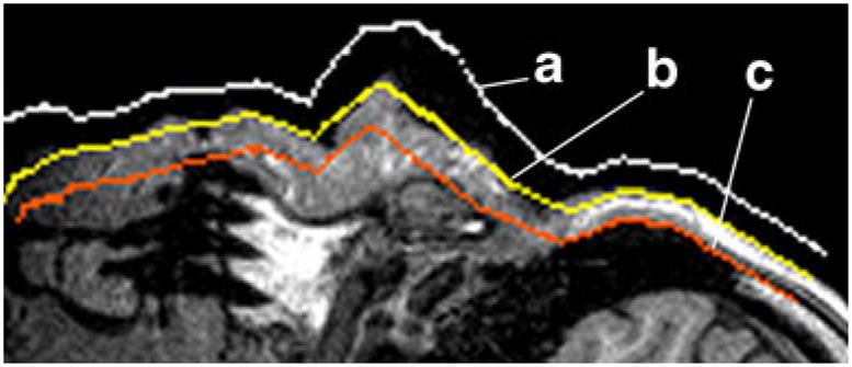
2D face ROI of an MR image with computed surface boundary for a “external” surface, b anatomical surface and c “deep” surface

To define the boundary layer, we enclose the triangulated anatomical surface (Fig. 1) in “interior” (deep) and “exterior” (superficial) tessellations (Fig. 2). These triangulated surfaces are obtained by translating each vertex of anatomical surface triangulation up or down the normal. The resulting boundary layer contains voxels roughly up to h mm deep under the skin, and shares the same parameterization (a function defining how coordinates on a surface depend on plane coordinates) with anatomical surface. (See Appendix for the mathematical derivation of anatomical surface parameterization).

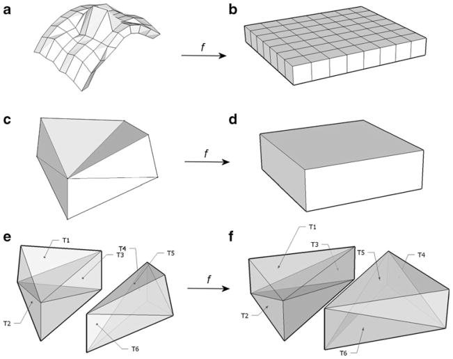
Corresponding deep and superficial triangulation vertices are connected by verticals, creating the partition of intermediate layer into oblique box-like blocks (quasi-blocks) with eight vertices and 12 triangular faces each, as illustrated on Fig. 3(a) and (c). Adjacent quasi-blocks share two triangular faces and four vertices. Each quasi-block can be consistently partitioned into six tetrahedrons (Fig. 3(e)), allowing geometric query whether any given voxel belongs to the boundary layer or not. To establish that, it is sufficient to determine whether the voxel belongs to any tetrahedron that constitute the boundary layer. (For detailed mathematical description of quasi-block partition, refer to Appendix).

Fig. 3.

a boundary layer partition L, b rectangular box partition L̂, c, d quasi-block Ω and corresponding regular block Ω̂, e, f tetrahedral partitions of Ω and Ω̂

Masking of the Boundary Layer

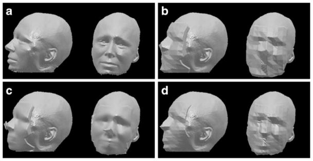
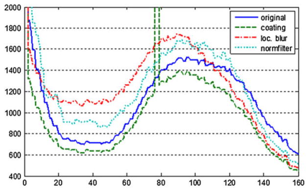
The boundary layer isolated in the previous step (Fig. 3a) contains all voxels to be modified in the original scan. The simplest choice to mask the enclosed surface would be to set all voxels within this layer to a fixed constant, such as average value. This technique, termed fill coating, effectively replaces the anatomical surface with the exterior or the interior tessellation (Figs. 4b and 5b). This approach removes all information from the boundary layer and introduces a single peak at pre-set intensity in the masked volume (Fig. 6). This peak can interfere with subsequent histogram analysis and may increase segmentation and shape reconstruction analysis errors.

Fig. 4.

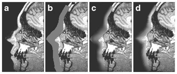
Effect of various masking methods on an MR slice. a unmodified, b fill coating, c localized blur, d normalized filtering

Fig. 5.

Surface renderings of a unmodified MR head acquisition, b modified by fill coating, c localized blur, d normalized filtering

Fig. 6.

Histograms of a head T1 acquisition: unmodified original (solid line) and masked (interrupted lines) with fill coating, localized blur, and normalized filtering

To make the transition between modified and non-modified anatomical surface less drastic, we also tried another approach termed localized blur. With this method, an averaging filter is applied to a copy of the original scan, and then only voxels within the boundary layer are replaced by those from the blurred volume (Figs. 4c and 5c).

Since in the case of localized blur the entire volume is averaged, outside voxels still contribute to actual values inside the boundary layer. A typical lowpass filter increases local continuity in voxel intensities by replacing each voxel with a weighted sum of its neighbors. Therefore, we can expect jumps in intensity along the edges of the boundary layer. This is indeed noticeable on Fig. 4c, where bright fat signal is averaged with dark bone and background signal from voxels outside the boundary layer, giving distinct greyish/white edge to the deep surface of the boundary layer. We also found that histograms of volumes processed with localized blur often show a noticeable shift in peak signal intensities, as illustrated on Fig. 6.

To mitigate the shortcomings of localized blur filtering, we formulated the following requirements to the ideal boundary layer degradation filter: a) continuity: signal jump at the interface between the boundary layer across deep surface and internal tissue should be minimal; b) tangentiality: voxels near the anatomical surface should be the result of averaging with other voxels near the surface, and the contribution of other types of voxels (much deeper or much higher above the surface) should be minimal. The latter condition simply requires that surface degradation is performed mainly along directions tangent rather than normal to the surface, so that more information pertaining to the surface is removed and less information pertaining to deeper tissues is altered or used for calculation of boundary layer voxels (see Fig. 7 for the illustration of the summation direction for a two-dimensional image).

Fig. 7.

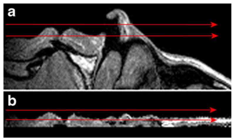
Arrows show the lines along which voxel values are averaged in case of a original, b “flattened” anatomical surface

Tangentiality is equivalent to including more voxels near the surface and less “external” or “deep” voxels in calculating the final voxel value. To model that, we used the filter kernel shape resembling a shallow box, with width and height much higher than depth. At the same time, the orientation of this box depends on the surface normal, whereas averaging directions for localized blur are co-aligned with volume’s natural coordinate system. A direct approach to ensure tangentiality would be to implement a filter with oblique neighborhood summation directions dependent on voxel position. If done directly, this would require multiple interpolations along these directions at each voxel, requiring impractical implementation complexity and computation time. Another approach would be to “flatten” the boundary layer to the coordinates where the normal at each vertex of triangulation does not change. Doing this for every voxel may be impractical, but if we assume the surface normal to be constant within every quasi-block, the problem reduces to transforming quasi-block into right-angled (proper) block, as detailed in the next section.

Boundary Layer Projection

In order to enable tangential smoothing, quasi-blocks produced in the tessellation steps above can be transformed to a regular flat rectangular box (a proper block) (Fig. 3a and b). A convolution filter is applied to this transformed mesh in directions tangent to the average anatomical surface or perpendicular to it, satisfying both the continuity and tangentiality conditions. This transformation of the irregular tessellated boundary layer is called here normalization, to indicate “normal” conditions for applying a degrading filter to the boundary layer.

Normalization transforms a layer of voxels onto another layer of voxels. As internal and external surface meshes of the boundary layer are parameterized by rectangular coordinates (Fig. 1), the same coordinates can be used to parameterize “external” and “internal” surfaces for the target flat box (Fig. 3b). Thus, there is one-to-one correspondence between each quasi-block and proper block in the target (Fig. 3c and d). Therefore, all we need is to find a transform between (c) and (d) on Fig. 3, and then combine for all blocks to perform normalization.

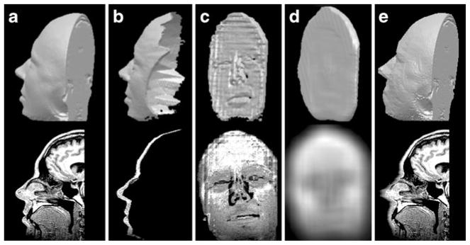
Since each quasi-block has 8 distinct vertices, both oblique and regular boxes can be partitioned into six tetrahedrons (Fig. 3e and f). For the actual transform, we pre-compute six affine transforms for each tetrahedral pair. Then, for each voxel in the target box, we find the tetrahedron it belongs to, and obtain the source voxel by applying a precomputed inverse affine transform for this tetrahedron to the voxel coordinates. By repeating this for all boxes in the target, the entire boundary layer is transformed (normalized). Figure 8b and c illustrates an isolated 3D surface rendering of a boundary layer and its projection onto the flat box.

Fig. 8.

Intermediate steps of normalized filtering applied to a T1 head acquisition (face ROI is shown). a volume of interest, b boundary layer (sagittal), c normalized boundary layer (coronal), d filtered boundary layer (coronal), e inverse transform of the filtered layer to the original volume (sagittal). Upper row: 3D surface rendering, lower row: a middle 2D slice from the volume

Normalized Filtering

If an averaging filter much wider in X and Y (right-left and top-bottom in the case of a face) directions than in Z (shallow-deep) direction is applied to the normalized boundary layer, more voxels from the nearby anatomical surface will contribute to the resulting voxel value than from voxels high above or deep below the surface, satisfying the tangentiality condition from “Masking of the boundary layer”. To satisfy the continuity condition, we used an averaging filter with variable kernel width. The kernel size was set to vary smoothly with depth below the surface, which resulted in smaller blur at the interface between the detected boundary layer and unmodified voxels.

The averaged layer is projected back to the original volume using the same “normalization” process of transforming a tetrahedral partition of a “flat” layer onto an equivalent tetrahedral partition of the original boundary layer (see Appendix). The algorithm that performs boundary layer projection, anisotropic filtering, and back-projection to the original volume is termed here normalized filtering. The result of each step of the normalized filtering applied to a T1 head acquisition is shown on Fig. 8.

Evaluation and Results

Face Masking Pipeline and Testing Datasets

We have implemented fill coating, localized blur and normalized filtering of the surface layer as MATLAB functions². At the initial step, the object binary mask is generated using automatic object/background thresholding (Ridler and Calvard 1978). The resulting mask is morphologically closed with 2 mm spherical kernel to simplify surface topology and reduce random noise, after which control is passed to the boundary layer generation routine.

These generic MATLAB functions can be applied to any external anatomical surface region. They require the coordinates of the box-like ROI and the coordinate axis perpendicular to the anatomical surface. In order to automatically obscure a face on MR head scan, we developed an automatic pipeline based on Linux shell scripts that first registers the volume to an atlas space using an in-house global 12-parameter affine transform optimization (Rowland et al. 2005).³ We used normal adult post-gadolinium contrast atlas as a target for selecting face ROI and pre-calculated a generous ROI containing face region in atlas space. The boundaries of this ROI are transformed to the original image space to automatically determine the input coordinates. As a result, the defacing pipeline does not require any input parameters.

MR Data

To validate the code, each of the three surface masking techniques was automatically applied to over 300 T1 and T2 weighted MR head volumes obtained using various sequences with approximately 1×1×1 mm or smaller voxel size and 3T magnetic field strength. Further comparison and numerical analysis described below was done on 16 randomly selected subjects, with age ranging from 10 to 88 and randomized disease state. Surface obscuring results are illustrated on Figs. 4 and 5. According to automatic parameter selection within the defacing pipeline, typical proper block size was 15×15 mm (left to right and top to bottom) and layer thickness (block depth) was 9 mm. For all methods, we used averaging filter. For the localized volume blur, filter neighborhood size was auto-selected to be 20×20×20 mm; and for the normalized anterior filtering, the size typically ranged from 10×10×3 mm at the deepest point to 30×30×10 mm at anatomical surface and above. The average running time per volume on a 2.8 GHz 64 bit processing node for localized blur and anterior coating was about 60 s, and 100 s for normalized filtering. Two reviewers visually inspected each of the 300 processed volumes to understand 1) alteration to the facial surface by comparing surface renderings of the original and processed volumes; 2) “invasiveness” into brain tissues; 3) how much of the perceived anatomical surface was captured inside the generated boundary layer. Both reviewers agreed that surface degradation was significant and uniform across most cases, with a few outliers that showed significant deviation in morphology from the rest and could possibly be identified by non-facial features such as general head shape. A number of cases also showed invasion of altered voxels into the nervous tissue, particularly in subjects with unusually thin frontal bone and meninges. To compensate for this misbehavior in the later versions of the automatic processing, we prohibited brain voxel alterations using pre-calculated brain mask (Smith 2002). Finally, boundary layer extraction captured facial surface properly in all cases except for acquisitions with high bias of MR signal, where both actual threshold and signal-to-noise ratio in the inferior facial region could drop by as much as 300 % compared to the superior. In these volumes, the boundary layer could “slip” under the actual anatomy. Our current experiments show that using multiple region-specific thresholds for anatomical surface generation helps to improve the accuracy of captured boundary layer.

We also compared the impact of boundary layer degradation techniques on certain image statistics and MR analysis tools, as discussed in the next section. The pre- and post-modified data for sample cases can be accessed at https://central.xnat.org/data/projects/surfmask_smpl.

CT Data

We applied normalized filtering to facial areas of 25 full body CT scans with voxel resolution 1×1×1 mm. The effect of normalized filtering on a CT acquisition is shown on Fig. 9.

Fig. 9.

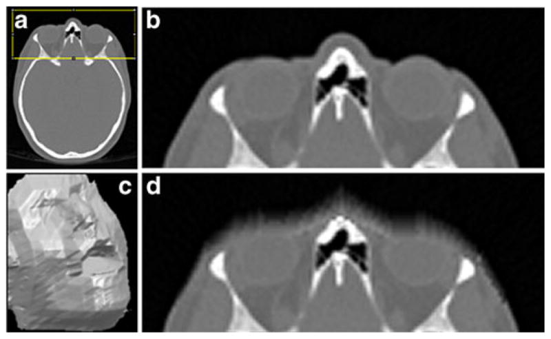
CT head acquisition modified by normalized filtering. a 2D axial slice with marked face ROI, b 2D slice from the face ROI, c surface rendering of the volume masked with normalized filtering, d filtered 2D slice from (b)

Impact of Surface Degradation on Image Statistics and Processing Tools

In this section, we consider several imaging metrics and how they change after application of face masking. For all statistical comparisons, we used Kolmogorov-Smirnov test for normality of distribution with unknown parameters (Lilliefors 1967). For normally distributed samples, paired t-test was used for comparison between different methods. When sample data did not pass normality test, we used Wilcoxon signed rank test.

The first test was to compare similarity between original and face surface masked (or simply masked) volumes. We used 16 pairs of unmodified and masked MR images for quantitative evaluation. MR data was chosen because of good contrast of soft tissues and availability of MR processing tools. For similarity measures, we used normalized mutual information (NMI) and average pixel distance (APD). NMI is widely used in image registration problems as a measure of how well two images are aligned (Collignon et al. 1995; Wells III et al. 1996). In our case, normalized mutual information indicates how much orientation information is preserved after applying the volume masking. A higher NMI with the original volume implies that atlas registration methods based on mutual information calculation, for example, would perform better.

Average NMI between original and surface-degraded versions for the 16 MR head volumes is shown in Table 1, first row. We tested the null hypothesis that NMI for normalized filtering is not statistically different from NMI for coating and blur. The p value for both cases was below 0.001, indicating that normalized filtering maintained the highest NMI with statistically significant difference.

Table 1.

The effect of different volume obscuring methods on results of selected skull stripping and gain field correction methods for sixteen evaluated MR head volumes. Notations: NMI - normalized mutual information; APD - average pixel distance. Statistical test p values indicate probability that the null hypothesis (i.e. the method for this column is not statistically different from the normalized filtering) is true

Applied processing	Similarity measure	Localized blur		Fill coating		Normalized filtering
		Mean	Statistical test	Mean	Statistical test	Mean
Original volume	NMI between the original and masked volumes	0.075	paired t, p = 5e-8	0.074	paired t, p = 4e-8	0.076
	APD between the original and masked volumes	11.1	paired t, p = 2e-6	14.3	paired t, p = 2e-8	9.2
Skull stripping	Volume overlap between the skull-stripped original and masked volumes	99.2 %	Wilcoxon signed rank, p = 4e-4	99.2 %	Wilcoxon signed rank, p = 3e-3	99.4 %
MR gain field correction	APD between the corrected original and masked volumes	0.42	Wilcoxon signed rank, p = 0.04	0.37	Wilcoxon signed rank, p = 0.09	0.33

The Average Pixel Distance APD between images A and B is described by the quantity

$$\mathit{APD}(A,B)={\left(\frac{1}{N}\sum _{i=1}^N{(a_i-b_i)}^2\right)}^{1/2}.$$ (1)

This integrative measure is useful to show the degree of localized intensity difference between two grayscale images. Since in all our tests the original and masked images were perfectly aligned, the pixel difference for unaffected voxels did not contribute to the sum. The APD between the original and masked images therefore provides a measure of volume change confined to the boundary layer. Again we hypothesized that this difference for images processed with normalized filtering is not different from those processed by localized blur and coating. The probability (p value) to see this in the observed data was below 0.001, suggesting that normalized filtering on average maintains higher intensity similarity with the original images (Table 1, second row).

To study the effect of surface degradation on typical MR processing tools, we applied commonly used skull stripping (Smith 2002) and MR gain field correction (Zhang et al. 2001) algorithms to original and masked images. For the resulting brain binary masks, we computed the volume overlap

$$J(A,B)=\mid A\cap B\mid /\mid A\cup B\mid ,$$ (2)

also known as Jaccard similarity index (Table 1, third row). This reflects the ratio of voxels that are different to the total number of voxels in the brain mask. If surface degradation did not affect the performance of skull stripping, volume overlap of skull-stripped images based on original and masked versions should be close to 100 %. In practice, this overlap was above 99 % for all masking methods, with normalized filtering maintaining highest average overlap (99.4 %). In statistical comparison, we tested the assumption that overlap of BET-processed images based on localized blur and coating was not different from the overlap based on normalized filtering. P values for this assumption were 1e-5 and 1e-3, accordingly, suggesting that normalized filtering maintained the highest overlap. In other words, brain masks generated from images processed with normalized filtering were closest to brain masks generated from unmodified images.

Finally, to compare the results of gain field correction, we estimated APD between original and corrected volumes (Table 1, bottom row). Using the same statistical test on the results showed that selection of one or the other masking algorithm produced a less significant effect on the result of gain field correction algorithm, which can be explained by the fact that this algorithm makes most use of white and gray matter voxels unaffected by the de-identification preprocessing.

Discussion

Previous research (Prior et al. 2009; Chen et al. 2007; Budin et al. 2008) on our ability to recognize MR or CT datasets as belonging to a specific individual based on head surface renderings indicates that such renderings are poor substitutes for photographs, although chances for such recognition are higher than random. It is hard to model conditions for potential person identification under which MR or CT images are shared for analysis; forced choice recognition evaluation used in studies represents somewhat simpler recognition problem, whereas in real situation one may have to compare a surface rendering with images from memory. The extent of human ability to recognize a head surface rendering still remains unclear; but in the context of research data sharing, addressing subject privacy by modifying the original data can potentially interfere with accurate data analysis. Local surface deformation is less invasive compared to other de-identification methods that entirely delete the face and is therefore less likely to interfere with image analysis. Yet it still reduces the recognition rate, which is confirmed by results obtained by Budin et al. (2008). Our approach to boundary surface deformation based on filtering of the “flattened” boundary surface layer provides a framework for studying the effects of different kinds of surface modification on visual appearance of modified surface renderings, image statistics and processing tools.

Face masking cannot be reversed with deconvolution methods. In normalized filtering, we are using averaging filter, which, similar to motion blur filter, largely eliminates high frequencies from image. The algorithm uses filter sizes between 20 and 50 for 256×256 slices, which will amplify any random noise to suppress signal beyond possibility of restoration. (This is illustrated in Jahne 1997 for frequency domain). Additionally, any attempt of deconvolution using unaltered voxels on the boundary with altered mask will meet two obstacles. First, normalized filtering doesn’t use unaltered voxels in computation of altered ones, so knowledge of boundary intensities would be irrelevant. Second, variability in MR signal from superficial to deep areas in the head is too high to predict based on low-frequency data. In areas near brain, for instance, two or more of epidermis, cranium, CSF and meninges, is crossed when we sample MRI intensities in depth from skin surface. The intensity vs. traveled distance curve will have several spikes that are not possible to predict based on closest internal unaltered voxels, and during deconvolution any small error in prediction will be multiplied many times, suppressing useful signal.

The presented algorithm requires face region of interest coordinates input. To automatically generate this ROI, we perform pre-registration to a normal MR T1 post-gadolinium adult brain atlas. Since the initial atlas-based face ROI is quite generous (it includes about 1/3 of the frontal head), registration error up to a few millimeters is acceptable for the input ROI. We found this atlas suitable for both normal adults and tumor patient data that we used. A different target atlas may be preferable for age-specific or disease-specific population.

The results of testing of three different boundary layer modification approaches suggest that post-processing tools, such as skull stripping, can be sensitive to even slight changes in voxel intensity distribution. Closeness measures of original and modified volumes correlate with accuracy of skull stripping with high significance. Anisotropic filtering of the “flattened” surface layer resulted in higher volume similarity and accuracy of post-processing tools compared to two other techniques.

It has been demonstrated that the boundary surface deformation can be used to protect privacy of research patients (Budin et al. 2008). This work describes a new method for localized surface filtering that works with MR and CT volumes, and can incorporate different boundary filtering techniques. Our hope is that this work will provide a helpful tool for de-identification and illustrate the use of some quantitative performance measures for volume de-identification tools.

Information Sharing Statement

The MATLAB source code of the algorithm, distributed under the BSD open source license, can be downloaded from https://bitbucket.org/mmilch01/surfacemask. Instructions on setting up the environment to use surface masking combined with automatic registration with FSL software should be sought under the “Face masking” section at http://nrg.wustl.edu/software/. Examples of MR data processed with the face masking algorithm can be accessed at https://central.xnat.org/data/projects/surfmask_smpl. The face masking pipeline that can be integrated with the open source imaging research database toolkit XNAT (eXtensible Neuroimaging Tool-kit, Marcus et al. 2007b) can be acquired from https://marketplace.xnat.org/plugins/.

Appendix

Generating the “internal” and “external” Surfaces

Given the original volume V with dimensions {m, n, k}, we can represent an anatomical surface S as a height field F⁰(x,y) over plane XY (Fig. 1). Using ray casting with discrete step w along X and Y axes, values of F are obtained in points

$$\begin{array}{l}{F}_{i,j}^0=F^0(iw,jw),i=0,\dots ,[m/w]-1,j\\ =0,\dots ,[n/w]-1.\end{array}$$ (3)

Denoting for $s_{i,j}^0$ a vertex with coordinates $\left(iw,jw,F_{i,j}^0\right)$ belonging to an anatomical surface, a “natural” triangulation T of S⁰ composed of triangles $T_{ij}^1=(s_{i,j},s_{i,j+1},s_{i+1,j})$ and $T_{ij}^2=(s_{i,j+1},s_{i+1,j+1},s_{i+1,j})$ can be selected (Fig. 10). Using T, it is now possible to describe the thin layer L that encloses anatomical surface and has roughly constant thickness. For that purpose, we construct triangulation meshes T^t and T^b of “external” S^t (“above” S) and “deep” S^b (“below” S) surfaces. Noting that ${\displaystyle \sum _{k=1}^4}{(-1)}^k{n}_{i,j}^k=0$, an averaged unit normal n̄_{i, j} at this vertex is computed as

Fig. 10.

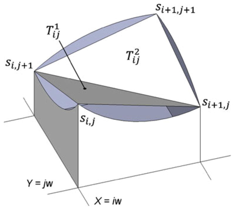
Triangulation S of the anatomical surface S⁰

$${\overline{n}}_{i,j}=\left(n_{i,j}^1+n_{i,j}^3\right)/\Vert n_{i,j}^1+n_{i,j}^3\Vert ,$$ (4)

where $n_{i,j}^k$, k = 1, …, 4 are outer unit normals of four triangular faces Θ¹,…, Θ⁴ of T that have a common vertex (Fig. 11).

Fig. 11.

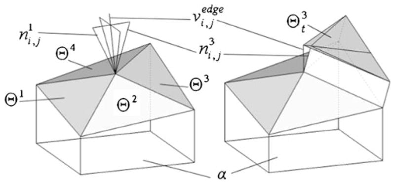
The average normal in vertex S_i,j (left) and construction of upper triangulation Θ_t (right)

If we travel a fixed distance h along n̄_{i, j} in “outer” (“upward”) direction, we will arrive at a vertex of the “external” triangulation T^t sharing the XY parameterization with T, and similarly for “internal” surface triangulation T^b:

$$s_{i,j}^t=s_{i,j}+v_{i,j}^{\mathit{edge}},s_{i,j}^b=s_{i,j}-v_{i,j}^{\mathit{edge}},$$ (5)

where

$$v_{i,j}^{\mathit{edge}}=\frac{1}{4}h{\overline{n}}_{i,j}\sum _{k=1}^4\frac{1}{({\overline{n}}_{i,j},n_{i,j}^k)}.$$ (6)

Thus, T^t and T^b are fully determined by (9–10). Since these surfaces have triangular faces that are nearly parallel to the corresponding faces of S, the thickness of L is maintained about 2h.

Boundary Volume Projection

The purpose of this derivation is to describe projection of L onto “thin” rectangular volume L̂ with dimensions m×n×h (Fig. 3b). Consider the quasi-block Ω_{i, j} formed by two space quadrilateral faces of S^t and S^b(Fig. 12). Each Ω_i,j can be consistently partitioned into six tetrahedra, as illustrated on Fig. 3e and f. Since cuboid box is an instance of octahedral element, establishing one-to-one correspondence between quasi-block Ω_{i, j} and a proper block Ω̂_{i, j} is equivalent to establishing correspondence between each pair of matching tetrahedra.

Fig. 12.

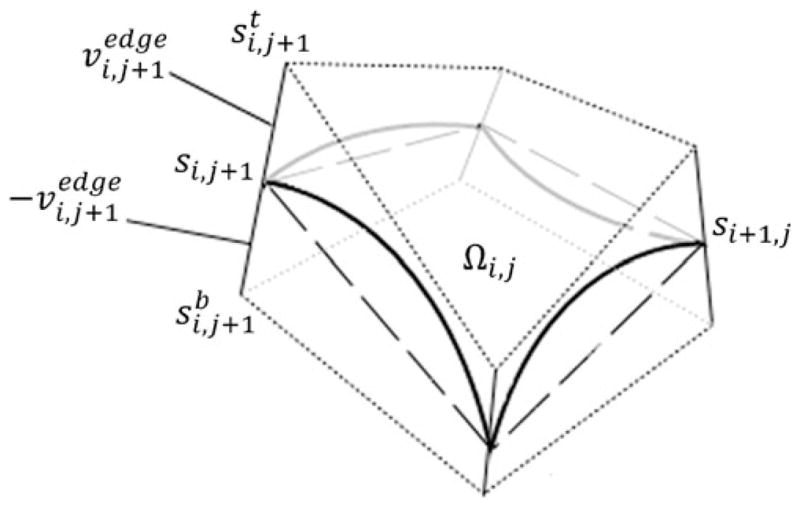
Quasi-block partition element Ω_{i, j} of the anterior layer L

Combining all transformed boxes together constitutes the new “flattened” rectangular volume L̂ (Fig. 3). Thus, one-to-one correspondence between L and is established via piecewise linear transform.

Consider the box volume L̂ with dimensions m×n×h (Fig. 3b). Consider the partition of L̂ into proper blocks Ω̂_i,j, where indices i and j have the same meaning as in Figs. 10, 11 and 12. Our aim is to establish a transformation f between these partitions such that:

$$f(L)=f(\cup {\mathrm{\Omega }}_{i,j})=\cup f({\mathrm{\Omega }}_{i,j})=\cup {\stackrel{⌢}{\mathrm{\Omega }}}_{i,j}=\stackrel{⌢}{L}.$$ (7)

Since each Ω_{i, j} has eight vertices, it is possible to partition it into six tetrahedra $T_{i,j}^1,\dots ,T_{i,j}^6$ (As illustrated on Fig. 3e), and because there is a one to one correspondence between ω_{i, j} and ω̂_{i, j}, a matching tetrahedral partition ${\stackrel{⌢}{T}}_{i,j}^1,\dots ,{\stackrel{⌢}{T}}_{i,j}^6$ can be also selected for ω̂_{i, j} (Fig. 3f) and matching affine transformation $f_{i,j}^k:T_{i,j}^k\to {\stackrel{⌢}{T}}_{i,j}^k$ be computed. Since ω_{i, j} provides a partition of L, combining individual affine transformations $f_{i,j}^k$ for each pair of ${\mathrm{\Omega }}_{i,j}^b$ and ω_{i, j} (Fig. 3c and d) will define a continuous non-degenerate piecewise linear transformation f between L and L̂:

$$f(L)=\underset{i,j}{\cup }f({\mathrm{\Omega }}_{i,j})=\underset{i,j}{\cup }\underset{k}{\cup }{f}_{i,j}^k(T_{i,j}^k)=\underset{i,j}{\cup }{\stackrel{⌢}{\mathrm{\Omega }}}_{i,j}=\stackrel{⌢}{L}.$$ (8)

Denoting the 4×4 affine transformation matrix from $T_{i,j}^k$ to ${\stackrel{⌢}{T}}_{i,j}^k$ for $A_{i,j}^k,f_{i,j}^k$ for an arbitrary point $P(\begin{array}{cccc}{x}_p& y_p& z_p& 1\end{array})$ in ω_{i, j} can be expressed as

$$f_{i,j}^k(P)=A_{i,j}^k(\begin{array}{cccc}{x}_p& y_p& z_p& 1\end{array}),P\in T_{i,j}^k$$ (9)

Coefficients of $A_{i,j}^k$ are calculated from the system of 12 linear equations with 12 unknowns matching the vertices of T_k and $T_k^b$. Once this transform is calculated, intensities in target tetrahedron $T_k^b$ are assigned by discrete 3D scanline filling (Kaufman and Shimony 1987) of its bounding box, and applying ${\left(A_{i,j}^k\right)}^{-1}$ to each voxel that is determined to be inside of $T_k^b$ to find the matching voxel in T_k. Thus, for transformation from L to L̂, the following discrete stepping procedure is applied:

1. For each Ω_{i, j}, do steps b–d:

2. for each k, form a system of 12 equations expressing the affine transform for each member tetrahedron of Ω_{i, j};

3. Determine an affine transformation matrix $A_{i,j}^k$ and its inverse ${\stackrel{⌢}{A}}_{i,j}^k={\left(A_{i,j}^k\right)}^{-1}$;

4. For each voxel in Ω̂_{i, j}, determine the matching tetrahedron ${\stackrel{⌢}{T}}_{i,j}^k$ (k can be one of 1,…,6) and find the corresponding voxel from $T_{i,j}^k$ using ${\stackrel{⌢}{A}}_{i,j}^k$, and set its intensity to the intensity of its prototype.

The transform back from L̂ to L is performed by scanning Ω_i,j instead of Ω̂_i,j, and following steps a–c, switching symbols with hat with symbols without hat.

References

- Bischoff-Grethe A, Ozyurt IB, Busa E, Quinn BT, Fennema-Notestine C, Clark CP, et al. A technique for the deidentification of structural brain MR images. Human Brain Mapping. 2007;28(9):892–903. doi: 10.1002/hbm.20312. [DOI] [PMC free article] [PubMed] [Google Scholar]
- Budin F, Zeng D, Ghosh A, Bullitt E. Preventing facial recognition when rendering MR images of the head in three dimensions. Medical Image Analysis. 2008;12(3):229–239. doi: 10.1016/j.media.2007.10.008. [DOI] [PMC free article] [PubMed] [Google Scholar]
- Chen J, Siddiqui K, Moffitt R, Juluru K, Kim W, Safdar N, Siegel E. Observer success rates for identification of 3D surface reconstructed facial images and implications for patient privacy and security. Proceedings of SPIE International Society for Optical Engineering. 2007:65161B-1–65161B-8. [Google Scholar]
- Collignon A, Maes F, Delaere D, Vandermeulen D, Suetens P, Marchal G. Automated multi-modality image registration based on information theory. Information Processing in Medical Imaging. 1995:263–274. [Google Scholar]
- Fennema-Notestine C, Ozyurt IB, Clark CP, Morris S, Bischoff-Grethe A, Bondi MW, et al. Quantitative evaluation of automated skull-stripping methods applied to contemporary and legacy images: effects of diagnosis, bias correction, and slice location. Human Brain Mapping. 2006;27(2):99–113. doi: 10.1002/hbm.20161. [DOI] [PMC free article] [PubMed] [Google Scholar]
- Jähne B. Digital Image Processing. Springer; 1997. p. 622. Retrieved from http://www.amazon.com/Digital-Image-Processing-Bernd-J%C3%A4hne/dp/3540240357. [Google Scholar]
- Jarudi IN, Sinha P. Relative Contributions of Internal and External Features to Face Recognition. 2003 Retrieved from http://dspace.mit.edu/handle/1721.1/7274.
- Jenkinson M, Smith S. A global optimisation method for robust affine registration of brain images. Medical image analysis. 2001;5(2):143–156. doi: 10.1016/s1361-8415(01)00036-6. Retrieved from http://www.ncbi.nlm.nih.gov/pubmed/11516708. [DOI] [PubMed] [Google Scholar]
- Kaufman A, Shimony E. 3D scan-conversion algorithms for voxel-based graphics. Proceedings of the 1986 workshop on Interactive 3D graphics - SI3D ’86; New York, New York, USA: ACM Press; 1987. pp. 45–75. [DOI] [Google Scholar]
- Lilliefors HB. Journal of the American Statistical Association. 62. Vol. 318. American Statistical Association; 1967. On the Kolmogorov-Smirnov Test for Normality with Mean and Variance Unknown; pp. 399–402. Retrieved from http://www.jstor.org/stable/2283970. [Google Scholar]
- Marcus DS, Wang TH, Parker J, Csernansky JG, Morris JC, Buckner RL. Open Access Series of Imaging Studies (OASIS): Cross-sectional MRI Data in Young, Middle Aged, Nondemented, and Demented Older Adults. Journal of Cognitive Neuroscience. 2007a;19(9):9. doi: 10.1162/jocn.2007.19.9.1498. [DOI] [PubMed] [Google Scholar]
- Marcus DS, Olsen TR, Ramaratnam M, Buckner RL. The Extensible Neuroimaging Archive Toolkit: an informatics platform for managing, exploring, and sharing neuroimaging data. Neuroinformatics. 2007b;5(1):11–34. doi: 10.1385/ni:5:1:11. [DOI] [PubMed] [Google Scholar]
- Mazura JC, Juluru K, Chen JJ, Morgan TA, John M, Siegel EL. Facial recognition software success rates for the identification of 3D surface reconstructed facial images: implications for patient privacy and security. Journal of Digital Imaging: the Official Journal of the Society for Computer Applications in Radiology. 2011 doi: 10.1007/s10278-011-9429-3. [DOI] [PMC free article] [PubMed] [Google Scholar]
- Prior FW, Brunsden B, Hildebolt C, Nolan TS, Pringle M, Vaishnavi SN, et al. Facial recognition from volume-rendered magnetic resonance imaging data. IEEE Transactions on Information Technology in Biomedicine: a Publication of the IEEE Engineering in Medicine and Biology Society. 2009;13(1):5–9. doi: 10.1109/TITB.2008.2003335. [DOI] [PubMed] [Google Scholar]
- Ridler TW, Calvard S. Picture Thresholding Using an Iterative Selection Method. IEEE Transactions on Systems, Man, and Cybernetics. 1978;8(8):630–632. doi: 10.1109/TSMC.1978.4310039. [DOI] [Google Scholar]
- Rowland DJ, Garbow JR, Laforest R, Snyder AZ. Registration of [18F]FDG microPET and small-animal MRI. Nuclear Medicine and Biology. 2005;32(6):567–572. doi: 10.1016/j.nucmedbio.2005.05.002. [DOI] [PubMed] [Google Scholar]
- Smith SM. Fast robust automated brain extraction. Human Brain Mapping. 2002;17(3):143–155. doi: 10.1002/hbm.10062. [DOI] [PMC free article] [PubMed] [Google Scholar]
- Wells WM, III, Viola P, Atsumi H, Nakajima S, Kikinis R. Multi-modal volume registration by maximization of mutual information. Medical Image Analysis. 1996;1(1):35–51. doi: 10.1016/S1361-8415(01)80004-9. [DOI] [PubMed] [Google Scholar]
- Zhang Y, Brady M, Smith S. Segmentation of brain MR images through a hidden Markov random field model and the expectation-maximization algorithm. IEEE Transactions on Medical Imaging. 2001;20(1):45–57. doi: 10.1109/42.906424. [DOI] [PubMed] [Google Scholar]