Quantitative Evaluation of Statistical Inference in Resting State Functional MRI

Abstract

Modern statistical inference techniques may be able to improve the sensitivity and specificity of resting state functional MRI (rs-fMRI) connectivity analysis through more realistic characterization of distributional assumptions. In simulation, the advantages of such modern methods are readily demonstrable. However quantitative empirical validation remains elusive in vivo as the true connectivity patterns are unknown and noise/artifact distributions are challenging to characterize with high fidelity. Recent innovations in capturing finite sample behavior of asymptotically consistent estimators (i.e., SIMulation and EXtrapolation - SIMEX) have enabled direct estimation of bias given single datasets. Herein, we leverage the theoretical core of SIMEX to study the properties of inference methods in the face of diminishing data (in contrast to increasing noise). The stability of inference methods with respect to synthetic loss of empirical data (defined as resilience) is used to quantify the empirical performance of one inference method relative to another. We illustrate this new approach in a comparison of ordinary and robust inference methods with rs-fMRI.

1 Introduction

When the brain is at rest (i.e., not task driven), functional networks produce correlated low frequency patterns of activity that can be observed with resting state fMRI (rs-fMRI). These correlations define one measure of functional connectivity which may be estimated by voxel-wise regression of activity in a seed region against that of the remainder of the brain [1]. The sensitivity and specificity of connectivity inference techniques hinge upon valid models of the noise in the observed data. Structured violations of the noise models due to local flow, bulk motion, distortions, or other artifacts can invalidate the methods traditionally used for inference [2]. Modern robust and non-parametric methods remain valid over a broader range of disturbances, but come with the cost of reduced power when the traditional methods would be appropriate. Therefore, a quantitative approach for comparing inference methods (and preprocessing pipelines leading to inference) is an essential analytical tool.

Several approaches for evaluating fMRI inference methods have been proposed. When repeated datasets are available, one can measure the reproducibility of estimated quantities when inference is applied to each dataset separately [3]. In task-based fMRI, cross-validation resampling procedures have been used to assess spatial patterns of reproducibility and temporal predictability for fMRI of task activities with the held-back samples [4]. More recent approaches for defining inference performance have considered the inference procedure as a classifier between the patterns of task activity and image intensity [5]. Yet, these advanced approaches are not applicable to rs-fMRI, and to date, no methods have been proposed to quantify relative performance of rs-fMRI inference methods based on typically acquired datasets (i.e., without large numbers of repeated scans for a single subject).

Herein, we propose a new inference comparison approach based on the resilience of the inference estimator. We apply this new technique to characterize ordinary and robust inference of rs-fMRI data. This approach does not require acquisition of additional data and is suitable for evaluation on isolated datasets as well as groups.

2 Theory

SIMEX is a statistical method that can be adapted to create resilience measures for inference in rs-fMRI. The principle behind SIMEX is that the expected value of an estimator diverges smoothly with increasing noise levels, therefore, the mean degree of corruption can be estimated by extrapolating a trend of divergence when synthetic noise is added to empirical data [6]. In our context, it is not reasonable to add noise because the noise distributions are uncertain — especially in the context of outliers. If we apply the SIMEX assumption of smooth convergence in this case, we can probe the marginal reduction in sensitivity of an estimator by removing data.

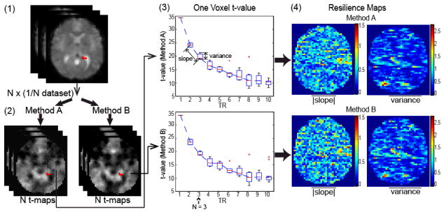
We define resilience as the ability of an inference method to maintain a consistent connectivity estimate despite a reduction in data. Over the time course of an rs-fMRI experiment (5–10 mins), the active brain regions vary. Hence, reproducibility of inferences based on sampled time periods is not meaningful. Therefore, we focus on decimating the sampling rate (Fig 1). The resilience of t-value estimates is quantified by two summary metrics: (i) the average absolute value of change in t-value with decimation level (i.e., slope), (ii) the average variance of the estimated metrics. The slope of t-value is computed by averaging the individual slopes between decimation levels.

Fig. 1.

Resilience features capture the stability of an inference method to data decimation. An rs-fMRI dataset (1) is temporally decimated into subsets; each inference method (2) is applied independently to each subset; voxel-wise statistics (3) are estimated; and the parameter maps (4) capture spatial dependencies.

2.1 Regression Models

rs-fMRI data can be analyzed with a first order autoregressive model, AR(1), for a weakly stationary time series [7],

$${\mathit{y}}_i=\mathbf{X}{\mathit{\beta }}_i+{\mathit{e}}_i,{\mathit{e}}_i~N(\mathbf{0},{\sigma }_i^2\mathit{V})$$ (1)

where y_i is a vector of intensity at voxel i, X is the design matrix, β_i is a vector of regression parameters at voxel i, and e_i is a non-spherical error vector. The correlation matrix V is estimated using Restricted Maximum Likelihood (ReML) and β is estimated on the whitened data (i.e., the “OLS” approach). Alternatively, a robust estimator (e.g., the “Huber” M-estimator [8]) may be applied after whitening. Both the OLS and Huber methods are available within the SPM software [9]. Herein, we used the Huber method with the tuning constant chosen for 95% asymptotic efficiency when the distribution of observation error is Gaussian distribution [10].

3 Methods and Results

3.1 One voxel simulation

Resilience aims to capture the performance of statistical inference methods on empirical data where the true correlations are unknown. If the true correlations are known, one could directly calculate the type I and type II errors. To explore how our definition of resilience relates to the type I error and the type II error, we performed single voxel simulation using an AR(1) model,

$$\mathit{y}={\beta }_{\mathbf{0}}+{\beta }_{\mathbf{1}}\mathit{x}+\mathit{e},\mathit{e}~N(\mathbf{0},V)$$ (2)

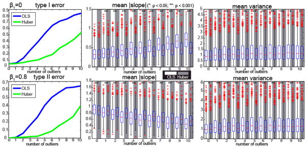
where x was simulated as region of interest (ROI) time course containing 200 time points with an approximately uniform distribution between 10 and 20 (arbitrary units), e was distributed as zero mean autoregressive Gaussian noise with standard deviation equaling 10% of the mean y value and normalized correlation 0.2. The null hypothesis H₀ : β₁ = 0 was tested using a t-test. In separate simulations, β₁ was assigned to 0 for specificity exploration and 0.8 for sensitivity exploration. The type I and type II errors are calculated based on p-value (p < 0.05). To simulate structured outliers, Rician distributed noise (Rice(0,25)) was added to the y values corresponding to values with the lowest or largest intensity. Rician noise is used to reflect the distribution of noise in MR magnitude images. The number of outliers was swept between 0 and 10 using 10³ Monte Carlo repetitions each. The covariance matrix was assumed to be known, and OLS and Huber inference were performed independently after whitening. Resilience metrics were calculated with three data partitions (degraded up to ¼ of the dataset). Fig. 2 compares type I error, type II error, and resilience as a function of number of outliers; significant differences were evaluated using the Wilcoxon signed-rank test.

Fig. 2.

One voxel simulation. Y axes are indicated by panel titles. The first row shows the results when and the second row shows the results when. When the number of outliers increases, the type I error and the type II error of OLS increases more rapidly than Huber M-estimator. The boxplots in the white background display the results from OLS and the boxplots in the gray background are the results from Huber M-estimator.

Both OLS and Huber controlled the type I and type II errors when there were no outliers. For the resilience, the mean absolute slope and the mean variance of OLS and Huber are not significantly different when β₁ = 0 without outliers. When β₁= 0.8 without outliers, the mean absolute slope from OLS is larger than Huber while the mean variance is smaller. These results are in agreement with the known behavior that robust methods are not as powerful as OLS when assumptions are met.

When considering outliers, Huber resulted in lower mean absolute slope and mean variance than OLS (for β= 0). When β = 0.8, the mean absolute slope of Huber was higher (due to higher t-statistics with all data), but Huber yield lower variance estimates. Hence, we must consider both the mean absolute slope and mean variance in consideration of estimator performance as these are complementary measures. The mean variance from OLS increases when outliers appear because some decimation samples include outliers while others do not. In contrast, Huber is more resistant to outliers so that the variances are relatively constant. The resilience results show less significance (e.g., last columns in the mean variance in Fig. 2) which is concordant with the decrease in the proportion of the differences in absolute errors. In summary, the resilience is strongly correlated with the type I and type II errors.

3.2 Empirical 3T rs-fMRI Experiment

Eleven rs-fMRI of healthy subjects were acquired at 3T using EPI (197 vol, FOV = 192 mm, flip θ = 90°, TR/TE = 2000/25 ms, 3×3×3 mm, 64×64×39 voxels) [11]. Prior to analysis, all images were corrected for slice timing artifacts and motion artifacts using SPM8 (University College London, UK). All time courses were low pass filtered at 0.1 Hz using a Chebychev Type II filter, spatially normalized to Talairach space, spatially smoothed with an 8 mm FWHM Gaussian kernel, linearly detrended, and de-meaned. Two voxels inside the right primary motor cortex for each subject were manually selected as the ROI by experienced researchers through exploring the unsmoothed images and comparing with the standard atlas. The design matrix for the general linear model was defined as the ROI time courses, the six estimated motion parameters, and one intercept. To create whole-brain connectivity maps, every labeled brain voxel underwent linear regression using the design matrix followed by a one sided t-test on the coefficient for the ROI time courses.

For each subject, the whole dataset (197 scans) was subsampled. First, the TR value was set to be 4 s (TR = 2 s in the original dataset), the 197 time series fMRI scans were divided into two subsamples, one containing 99 scans and the other containing 98 scans. Similarly, the TR value was set to be 6 s to obtain three subsamples. This procedure was repeated with a TR value of 8 s. Thus, we have one original dataset and three collections of subsampled datasets for each subject. The resting state fMRI analysis was performed on each dataset in SPM8 using OLS and Huber inference.

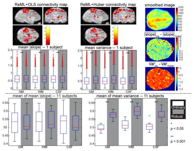
To quantitatively compare the resilience of these two methods, the mean absolute slope and the mean variance are evaluated across the gray matter (GM), white matter (WM) and cerebrospinal fluid (CSF). To evaluate all subjects, we calculated the mean of the mean absolute slope value and the mean of the mean variance in each brain region for each subject. The significance of differences between the ordinary and the robust estimation method were tested using the Wilcoxon signed-rank test.

The mean absolute slope and the mean variance from OLS are smaller than those of Huber (Fig. 3). Over the 11 subjects, the mean absolute slope of OLS is not significantly different while the mean variance is significantly smaller. Thus, the resilience metrics confirm expectations that OLS is a superior inference technique for high quality empirical data (i.e., when distributional assumptions are appropriate).

Fig. 3.

Resilience results for empirical 3T rs-fMRI analysis. The upper plots present results for a representative subject and the lower plots display the results across the 11 subjects. The first row shows the connectivity maps estimated by the OLS and Huber methods (p < 0.001, 5 voxels extent threshold to exclude noise). The blue crosshairs indicates one voxel inside the ROI. The right column displays one slice of the smoothed image from one scan (top) the difference of the mean absolute slope (middle), and the difference of the mean variance (bottom) for the same slice. The mean absolute slope and the mean variance from OLS (white background) and Huber (gray background) across GM, WM and CSF regions are shown in the second row. In the second half, the mean of the mean absolute slope and the mean of the mean variance across eleven subjects are displayed. Significant differences based on the Wilcoxon signed-rank test are indicated by the asterisks.

3.3 Empirical 3T rs-fMRI Experiments with Outliers

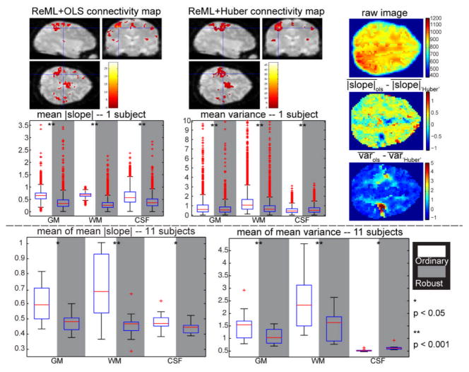
To illustrate the use of resilience in the presence of outliers, a dataset with outliers was simulated by increasing the WM intensity of the empirical 3T rs-fMRI dataset described in section 3.2. The simulation results show that three outliers are enough to tell the difference between OLS and Huber estimation so we selected three scans with low ROI intensity and added random positive noisy images inside the WM region to simulate outlier scans. Noisy Rician images are created with σ at 10% of the mean intensity and spatially smoothed at 8 mm FWHM Gaussian kernel. One slice of an outlier image is displayed in Fig. 4 (compare with Fig. 3).

Fig. 4.

Resilience results for 3T resting state fMRI with simulated outliers. The upper plots present the results for the same subject shown in Fig. 3 and the lower plots display the results across the 11 subjects. The first row shows the connectivity maps estimated by the OLS and Huber methods (p < 0.001, 5 voxels extent threshold to exclude noise). The right column displays (top) one outlier image from one scan for the same slice shown in Fig. 3, (top) the difference of the mean absolute slope and (bottom) the difference of the mean variance. The mean absolute slope and the mean variance from the ordinary and the robust method across GM, WM and CSF regions are shown in the second row. Below, the mean of the mean absolute slope and the mean of the mean variance across eleven subjects are displayed. Significant differences calculated with the Wilcoxon signed-rank test are indicated by asterisks.

We applied the same connectivity analysis method (OLS and Huber) and the same resilience calculation method (TR from 2s to 8s, mean absolute slope and mean variance in GM, WM and CSF) described in section 3.2 (Fig. 4).

The connectivity maps illustrate that the OLS method lost substantial power in the vicinity of the seed voxels when outliers were introduced whereas the Huber method preserved detection. In terms of resilience, the Huber approach resulted in significantly smaller mean absolute slope and mean variance in the WM. We also noted smaller mean absolute slope and smaller mean variance from the robust method than the ordinary method in GM regions. The relative improvement of the Huber performance in GM may due to the spatially pooled covariance estimation. In CSF, the mean absolute slope from OLS is larger while the mean variance is smaller for the example subject and across subjects. Noting that there are no outliers in the CSF it is reasonable that the performance of Huber is not better than OLS. The resilience results here suggest that the robust estimation method outperforms the OLS method if outliers are present.

4 Discussion

The proposed resilience metrics provide a quantitative basis on which to compare inference methods. The simulation results suggest that a comparison of methods based on resilience would yield similar conclusions as one based on the type I and type II errors. It is reassuring to see that resilience also indicates that OLS would outperform a Huber inference approach when the data quality is high (as in the publicly available dataset under study), whereas a Huber approach would outperform OLS in cases when outliers are present. As rs-fMRI is applied to ever more challenging anatomical targets (i.e., those requiring high spatial and temporal resolution and/or using ultra-high field imaging), the achievable signal to noise ratio decreases and the propensity for artifacts increases [12]. Hence, it is becoming increasingly more important to quantitatively determine which inference methods are appropriate.

In summary, we have presented a novel approach for quantifying inference methods based on empirical data. Herein, we evaluated the resilience of the ordinary (OLS) and a robust method (Huber) for both simulated and empirical data. Resilience provides a simple, but powerful method for comparing a proxy for accuracy of inference approaches in empirical data where the underlying true value is unknown. Continued exploration of metrics based on resilience criteria promises to provide a fruitful avenue for comparative characterization of inference stability and “quality.”

Note that if two inference methods yield different t-values when all data are considered, the one that has a higher starting t-value will have a higher mean absolute slope even if both methods degrade at the same rate. Hence, in the regions of true association (i.e., β ≠ 0), the variance measure is likely of greater interest as it reflects degraded inference consistency. Yet, in regions that lack an association (i.e., β = 0), the slope measure would reflect on anonymous changes in t-value which could be attributed to “non-robust” influences. Consideration of data-adaptive combinations of these metrics would be area of fruitful investigation.

References

- 1.van den Heuvel MP, Hulshoff Pol HE. Exploring the brain network: a review on resting-state fMRI functional connectivity. European neuropsychopharmacology: the journal of the European College of Neuropsychopharmacology. 2010;20:519–534. doi: 10.1016/j.euroneuro.2010.03.008. [DOI] [PubMed] [Google Scholar]
- 2.Penny WD, et al., editors. Statistical Parametric Mapping: The Analysis of Functional Brain Images. Academic Press; New York, NY: 2006. [Google Scholar]
- 3.Genovese CR, et al. Estimating test-retest reliability in functional MR imaging I: Statistical methodology. Magnetic Resonance in Medicine. 1997;38:497–507. doi: 10.1002/mrm.1910380319. [DOI] [PubMed] [Google Scholar]
- 4.Strother SC, et al. The quantitative evaluation of functional neuroimaging experiments: The NPAIRS data analysis framework. Neuroimage. 2002;15:747–771. doi: 10.1006/nimg.2001.1034. [DOI] [PubMed] [Google Scholar]
- 5.Afshin-Pour B, et al. A mutual information-based metric for evaluation of fMRI data-processing approaches. Human brain mapping. 2011;32:699–715. doi: 10.1002/hbm.21057. [DOI] [PMC free article] [PubMed] [Google Scholar]
- 6.Carroll RJ, et al. Measurement error in nonlinear models: a modern perspective. CRC Press; 2006. [Google Scholar]
- 7.Friston KJ, et al. Classical and Bayesian inference in neuroimaging: theory. NeuroImage. 2002;16:465–483. doi: 10.1006/nimg.2002.1090. [DOI] [PubMed] [Google Scholar]
- 8.Huber PJ, et al. Robust statistics. Wiley Online Library; 1981. [Google Scholar]
- 9.Yang X, et al. Biological parametric mapping with robust and non-parametric statistics. NeuroImage. 2011;57:423–430. doi: 10.1016/j.neuroimage.2011.04.046. [DOI] [PMC free article] [PubMed] [Google Scholar]
- 10.Holland PW, Welsch RE. Robust regression using iteratively reweighted least-squares. Communications in Statistics-Theory and Methods. 1977;6:813–827. [Google Scholar]
- 11.Shehzad Z, et al. The resting brain: unconstrained yet reliable. Cerebral cortex. 2009;19:2209. doi: 10.1093/cercor/bhn256. [DOI] [PMC free article] [PubMed] [Google Scholar]
- 12.Hutton C, et al. The impact of physiological noise correction on fMRI at 7T. Neuroimage. 2011 doi: 10.1016/j.neuroimage.2011.04.018. [DOI] [PMC free article] [PubMed] [Google Scholar]