Sparse Patch Based Prostate Segmentation in CT Images

Abstract

Automatic prostate segmentation plays an important role in image guided radiation therapy. However, accurate prostate segmentation in CT images remains as a challenging problem mainly due to three issues: Low image contrast, large prostate motions, and image appearance variations caused by bowel gas. In this paper, a new patient-specific prostate segmentation method is proposed to address these three issues. The main contributions of our method lie in the following aspects: (1) A new patch based representation is designed in the discriminative feature space to effectively distinguish voxels belonging to the prostate and non-prostate regions. (2) The new patch based representation is integrated with a new sparse label propagation framework to segment the prostate, where candidate voxels with low patch similarity can be effectively removed based on sparse representation. (3) An online update mechanism is adopted to capture more patient-specific information from treatment images scanned in previous treatment days. The proposed method has been extensively evaluated on a prostate CT image dataset consisting of 24 patients with 330 images in total. It is also compared with several state-of-the-art prostate segmentation approaches, and experimental results demonstrate that our proposed method can achieve higher segmentation accuracy than other methods under comparison.

1 Introduction

Prostate cancer is the second leading cause of cancer death for male in US. Image guided radiation therapy (IGRT), as a non-invasive approach, is one of the major treatment methods for prostate cancer. The key to the success of IGRT is the accurate localization of prostate in the treatment images such that cancer cells can be effectively eliminated by the high energy X-rays delivered to the prostate.

However, accurate prostate localization in CT images remains as a challenging problem. First, the image contrast between the prostate and its surrounding tissues is low. This issue can be illustrated by Figures 1 (a) and (b). Second, the prostate motion across different treatment days can be large. Third, the image appearance can be significantly different due to the uncertain existence of bowel gas. This issue can be illustrated by Figures 1 (a) and (c).

Fig. 1.

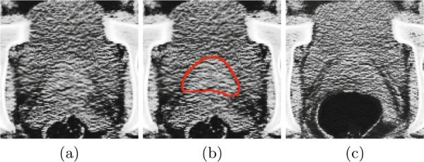
(a) An image slice of a 3D prostate CT image volume. (b) The manually delineated prostate boundary (i.e., the red contour) by the radiologist superimposed on the image in (a). (c) An image slice with bowel gas of a 3D prostate CT image volume with the same patient as in (a) but acquired from a different treatment day.

Many novel approaches have been proposed in the literature [1–4] for prostate segmentation in CT images. For instance, Davis et al. [1] proposed a deflation algorithm to eliminate the distortions brought by the existence of bowel gas, followed by a diffeomorphic image registration process to localize the prostate. Chen et al. [3] proposed a Bayesian framework for prostate segmentation in CT images. In this paper, we propose a new patient-specific prostate segmentation method. The main contributions of our method lie in the following aspects: (1) Anatomical features are extracted from each voxel position. The most informative features are selected by the logistic Lasso to form the new salient patch based signature. (2) The new patch based signature is integrated with a sparse label propagation framework to localize the prostate in each treatment image. (3) An online update mechanism is adopted to capture more patient-specific information from the segmented treatment images. Our method has been extensively evaluated on a prostate CT image dataset consisting of 24 patients with 330 images in total. It is also compared with several state-of-the-art prostate segmentation approaches, and experimental results demonstrate that our method achieves higher segmentation accuracy than other methods under comparison.

2 Patch Based Signature in Discriminative Feature Space

Patch based representation has been widely used in medical image analysis [5] as anatomical signatures for each voxel. The conventional patch based principle is to define a small K × K image patch centered at each voxel x as the signature of x, where K denotes the scale of interest.

However, the conventional patch based signature still may not fully distinguish voxels belonging to the prostate and non-prostate regions due to the low image contrast around the prostate boundary. Therefore, we are motivated to construct more salient patch based signatures in the feature space. For each image I(x), it is convolved with a specific kernel function ψ_j(x) by Equation 1:

$$F_j\left(\mathit{x}\right)=I\left(\mathit{x}\right)\ast {\psi }_j\left(\mathit{x}\right),(j=1,\dots ,L)$$ (1)

where F_j(x) denotes the resulting feature value with respect to the jth kernel ψ_j(x) at voxel x. L denotes the number of kernel functions used to extract features. In this paper, we adopt the Haar [6], histogram of oriented gradient (HOG) [7], and local binary pattern (LBP) [8] features.

For each feature map F_j(x) (j=1,…,L), we can also define a K × K patch centered at each voxel x. Thus, x has a K × K × L dimensional signature, denoted as a(x). Then, the logistic Lasso [9] is adopted to select the most informative features. More specifically, N voxels x_i (i=1,…,N) are sampled from the training images, with labels l_i = 1 if x_i belongs to the prostate and l_i = −1 otherwise. Then, we aim to minimize the logistic Lasso problem [10] in Equation 2:

$$J(\beta ,c)=\sum _{i=1}^N\text{log}(1+\text{exp}(-l_i({\beta }^T\alpha \left({\mathit{x}}_i\right)+c)))+\lambda {\Vert \beta \Vert }_1,$$ (2)

where β is the sparse coefficient vector, ‖ · ‖₁ is the L1 norm, c is the intercept scalar, and λ is the regularization parameter. The optimal solution β^opt and c^opt to minimize Equation 2 can be estimated by Nesterov's method [11]. The most informative features can be determined by selecting features with β^opt(d) ≠ 0 (d = 1, …, K × K × L). We denote the final signature of each voxel x as b(x).

3 Sparse Patch Based Label Propagation

The general label propagation process [5] can be formulated as follows: Given n training images and their segmentation groundtruths (i.e., label maps), denoted as {(I_u, S_u), u = 1, …, n}. For a new treatment image I_new, each voxel x in I_new is linked to each voxel y in I_u with a graph weight w_u(x, y). Then, the corresponding label for each voxel x can be estimated by Equation 3:

$$S_{\mathit{new}}\left(\mathit{x}\right)=\frac{\sum _{u=1}^n\sum _{\mathit{y}\in \Omega }{w}_u(\mathit{x},\mathit{y})S_u\left(\mathit{y}\right)}{\sum _{u=1}^n\sum _{\mathit{y}\in \Omega }{w}_u(\mathit{x},\mathit{y})},$$ (3)

where Ω denotes the image domain, and S_new denotes the prostate probability map of I_new.

Based on the new patch based signature derived in Section 2, the graph weight w_u(x, y) can be defined by Equation 4 similar to [5]:

$$w_u(\mathit{x},\mathit{y})=\{\begin{array}{cc}\Phi \left(\frac{\Vert {\mathit{b}}_{I_{\mathit{new}}}\left(\mathit{x}\right)-{\mathit{b}}_{I_u}\left(\mathit{y}\right){\Vert }_2}{2K\alpha }\right),\hfill & \mathrm{if}\mathit{y}\in {\mathcal{N}}_u\left(\mathit{x}\right);\hfill \\ 0,\hfill & \text{otherwise}.\hfill \end{array}\phantom{\}}$$ (4)

where b_Inew(x) and b_Iu(y) denote the patch signature at x of I_new and at y of I_u, respectively, and ‖ · ‖₂ denotes the L2 norm. The heat kernel Φ(x) = e^−x is used similar to [5]. α is the smoothing parameter. ${\mathcal{N}}_u\left(\mathit{x}\right)$ denotes the neighborhood of voxel x in image I_u, and it is defined as the W × W × W subvolume centered at x. Noted that the standard deviation of image noise for the selected features could also be considered in Equation 4 to estimate the graph weight more accurately.

Inspired by the discriminant power of sparse representation, we are motivated to estimate the graph weight based on Lasso. Specifically, we organize b_Iu(y), $\mathit{y}\in {\mathcal{N}}_u\left(\mathit{x}\right)(u=1,\dots ,n)$ as columns of a matrix A. Then, the sparse coefficient vector θ_x for voxel x is estimated by minimizing Equation 5 with Nesterov's method [11]:

$$J\left({\theta }_{\mathit{x}}\right)=\frac{1}{2}{\Vert {\mathit{b}}_{I_{\mathit{new}}}\left(\mathit{x}\right)-\mathbf{A}{\theta }_{\mathit{x}}\Vert }_2^2+\lambda {\Vert {\theta }_{\mathit{x}}\Vert }_1,{\theta }_{\mathit{x}}\ge 0.$$ (5)

We denote the optimal solution of Equation 5 as ${\theta }_{\mathit{x}}^{\mathit{opt}}$. The graph weight w_u(x, y) is set to the corresponding element in ${\theta }_{\mathit{x}}^{\mathit{opt}}$ with respect to y in image I_u.

Then, the prostate probability map S_new is estimated by Equation 3. Figure 2 shows an example of the prostate probability maps obtained by different strategies. It is shown that the new patch based signature with sparse label propagation estimates the prostate boundary more accurately.

Fig. 2.

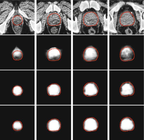
First row: original prostate CT images, overlayed with the groundtruth highlighted by red contours. Second to fourth rows: The corresponding probability maps obtained by label propagation with the intensity patch voxel signature, patch based voxel signature in the feature space without using sparse representation, and the patch based voxel signature in the feature space with sparse representation, respectively

After estimating the prostate probability map S_new, the prostate in I_new can be localized by aligning the segmentation groundtruth of each training image S_u (u = 1, …, N) to S_new and perform majority voting. The affine transformation [12] is used due to the relatively simple shape of the prostate.

4 The Online Update Mechanism

In this paper, an online update mechanism is adopted to incorporate more patient-specific information. More specifically, at the beginning stage of the radiation therapy, only the planning image of the current patient is available to serve as the training image. As more treatment images are collected and segmented during the therapy process, they will also serve as the training images. Therefore, the online update mechanism gradually captures more patient-specific information during the period of radiation therapy. It is worth noting that manual adjustments to the automatic segmentation results are also feasible to correct some poorly segmented images since such adjustments can be completed offline.

5 Experimental Results

Our method was evaluated on a 3D prostate CT dataset consisting of 24 patients with 330 images. Each image has in-plane resolution 512 × 512, with voxel size 0.98 × 0.98 mm². The voxel size along the sagittal direction is 3 mm. The segmentation groundtruth provided by the clinical expert is also available.

In all the experiments, the following parameter settings were adopted for our method by cross validation: patch size K = 5, neighborhood size W = 15, λ = 10⁻⁴ in Equations 2 and 5, α = 1 in Equation 4. Therefore, the dimension of the original feature is 1325, and the same subset of selected feature is used for all voxels. For each patient, we first rigidly aligned the pelvic bone structures of each treatment image to the planning image with FLIRT [12] to remove the whole-body rigid motion.

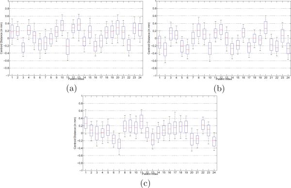
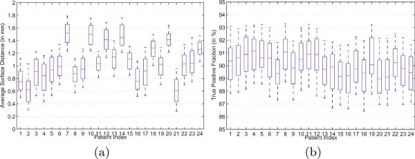
Four quantitative measures were used to evaluate the segmentation accuracy of our method: The centroid distance (CD), average surface distance (ASD), true positive fraction (TPF), and the Dice ratio. The whisker plots of CD along the lateral, anterior-posterior and superior-inferior directions of each patient are shown in Figures 3 (a) to (c), respectively. It is shown that the median CD along each direction of each patient lies within 0.4 mm from the groundtruth, which implies the effectiveness of our method. The whisker plots of the ASD and TPF measures of each patient are also shown in Figures 4 (a) to (b), respectively.

Fig. 3.

Centroid distance between the estimated prostate by our method and the groundtruth along the (a) lateral, (b) anterior-posterior, and (c) superior-inferior directions, respectively. The horizontal lines in each box represent the 25th percentile, median, and 75th percentile. The whiskers extend to the most extreme data points.

Fig. 4.

Whisker plots of the (a) average surface distance and (b) true positive fraction between our estimated prostate and the groundtruth for each patient. The horizontal lines in each box represent the 25th percentile, median, and 75th percentile. The whiskers extend to the most extreme data points.

The average Dice ratio and its standard deviation between the estimated prostate volume and the groundtruth for each patient after bone alignment, with and without the online update mechanism of our method are also shown in Figure 5. It is shown that our method can achieve high Dice ratios (i.e., mostly above 85%) even without the online update mechanism (i.e, only the planning image is served as the training data). The segmentation accuracies can be further improved with the online update mechanism (i.e., mostly above 90%).

Fig. 5.

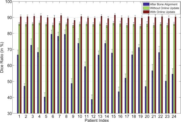
The average Dice ratios and the standard deviations of the 24 patients after bone alignment, and using our method without or with the online update mechanism.

A typical example of the segmentation results by using the proposed method is shown in Figure 6. It can be observed that the estimated prostate boundaries are very closed to the prostate boundaries of the groundtruth even for the apex area of the prostate and in slices where bowel gas exists.

Fig. 6.

Typical segmentation results of the 3rd treatment image of the 17th patient (first row, Dice ratio 90.04%) and the 5th treatment image of the 15th patient (second row, Dice ratio 90.86%). The yellow contours denote the estimated prostate boundaries by our method, and the red contours denote the prostate boundaries of the groundtruth.

Our method was also compared with three state-of-the-art prostate CT segmentation algorithms [1–3]. The best results reported in [1–3] were adopted for comparison, and detailed comparisons are listed in Table 1. It can be observed from Table 1 that our method outperforms other methods under comparison. The contributions of the new patch based signature and the sparse label propagation framework can also be mirrored by Table 1.

Table 1.

Comparison of different methods, N/A indicates that the corresponding result was not reported in the respective paper. The last three rows denote our method using intensity patch signature, discriminative (Dist) patch signature in feature space, and the discriminative (Dist) patch signature with sparse label propagation. Results obtained by our method on the last row are bolded.

Methods	Mean Dice Ratio	Mean ASD (mm)	Mean CD (x/y/z) (mm)	Median TPF
Davis et al. [1]	0.820	N/A	−0.26/0.35/0.22	N/A
Feng et al. [2]	0.893	2.08	N/A	N/A
Chen et al. [3]	N/A	1.10	N/A	0.84
Intensity Patch	0.731	3.58	1.84/1.62/−1.74	0.72
Dist Patch	0.862	1.52	0.24/−0.23/0.31	0.84
Our Method	0.909	1.09	0.17/−0.09/0.19	0.89

6 Conclusion

In this paper, we propose a new patient-specific prostate segmentation method for CT images. Our method extracts anatomical features from each voxel position, and the most informative features are selected by logistic Lasso to construct the patch based representation of in the feature space. It is shown that the new patch based signature can distinguish voxels belonging to the prostate and non-prostate regions more effectively. The new patch based signature is integrated with a sparse label propagation framework to localize the prostate in new treatment images. An online update mechanism is also adopted in this paper to capture the patient-specific information more effectively. The proposed method has been extensively evaluated on a prostate CT image dataset consisting of 24 patients with 330 images. It is also compared with several state-of-the-art prostate segmentation methods. Experimental results show that our method achieves higher segmentation accuracy than other methods under comparison.

References

- 1.Davis BC, Foskey M, Rosenman J, Goyal L, Chang S, Joshi S. Automatic Segmentation of Intra-treatment CT Images for Adaptive Radiation Therapy of the Prostate. In: Duncan JS, Gerig G, editors. MICCAI 2005. LNCS. vol. 3749. Springer; Heidelberg: 2005. pp. 442–450. [DOI] [PubMed] [Google Scholar]
- 2.Feng Q, Foskey M, Chen W, Shen D. Segmenting CT prostate images using population and patient-specific statistics for radiotherapy. Medical Physics. 2010;37:4121–4132. doi: 10.1118/1.3464799. [DOI] [PMC free article] [PubMed] [Google Scholar]
- 3.Chen S, Lovelock D, Radke R. Segmenting the prostate and rectum in CT imagery using anatomical constraints. Medical Image Analysis. 2011;15:1–11. doi: 10.1016/j.media.2010.06.004. [DOI] [PubMed] [Google Scholar]
- 4.Li W, Liao S, Feng Q, Chen W, Shen D. Learning Image Context for Segmentation of Prostate in CT-Guided Radiotherapy. In: Fichtinger G, Martel A, Peters T, editors. MICCAI 2011, Part III. LNCS. vol. 6893. Springer; Heidelberg: 2011. pp. 570–578. [DOI] [PMC free article] [PubMed] [Google Scholar]
- 5.Rousseau F, Habas P, Studholme C. A supervised patch-based approach for human brain labeling. IEEE TMI. 2011;30:1852–1862. doi: 10.1109/TMI.2011.2156806. [DOI] [PMC free article] [PubMed] [Google Scholar]
- 6.Mallat G. A theory for multiresolution signal decomposition: the wavelet representation. IEEE PAMI. 1989;11:674–693. [Google Scholar]
- 7.Dalal N, Triggs B. CVPR. 2005. Histograms of oriented gradients for human detection; pp. 886–893. [Google Scholar]
- 8.Ojala T, Pietikainen M, Maenpaa T. Multiresolution gray-scale and rotation invariant texture classification with local binary patterns. IEEE PAMI. 2002;24:971–987. [Google Scholar]
- 9.Tibshirani R. Regression shrinkage and selection via the lasso. Journal of the Royal Statistical Society: Series B. 1996;58:267–288. [Google Scholar]
- 10.Liu J, Ji S, Ye J. SLEP: Sparse Learning with Efficient Projections. Arizona State University. 2009 [Google Scholar]
- 11.Nesterov Y. Introductory Lectures on Convex Optimization: A Basic Course. Kluwer Academic Publishers. 2004 [Google Scholar]
- 12.Jenkinson M, Bannister P, Brady M, Smith S. Improved optimization for the robust and accurate linear registration and motion correction of brain images. NeuroImage. 2002;17:825–841. doi: 10.1016/s1053-8119(02)91132-8. [DOI] [PubMed] [Google Scholar]