Abstract
There has been discrepancies between the daily air quality reports of the Beijing municipal government, observations recorded at the U.S. Embassy in Beijing, and Beijing residents’ perceptions of air quality. This study estimates Beijing’s daily area PM2.5 mass concentration by means of a novel technique SPA (Single Point Areal Estimation) that uses data from the single PM2.5 observation station of the U.S Embassy and the 18 PM10 observation stations of the Beijing Municipal Environmental Protection Bureau. The proposed technique accounts for empirical relationships between different types of observations, and generates best linear unbiased pollution estimates (in a statistical sense). The technique extends the daily PM2.5 mass concentrations obtained at a single station (U.S. Embassy) to a citywide scale using physical relations between pollutant concentrations at the embassy PM2.5 monitoring station and at the 18 official PM10 stations that are evenly distributed across the city. Insight about the technique’s spatial estimation accuracy (uncertainty) is gained by means of theoretical considerations and numerical validations involving real data. The technique was used to study citywide PM2.5 pollution during the 423-day period of interest (May 10, 2010 to December 6, 2011). Finally, a freely downloadable software library is provided that performs all relevant calculations of pollution estimation.
Introduction
Beijing, the capital city of China, is an international metropolis with a population of over 19 million. As in many big cities worldwide, air pollution is a major concern for city residents. Particulate matter (PM) is the air pollutant that most commonly affects people’s health, where PM10 and PM2.5 are the two main PM pollutants, i.e., PM consisting of particles with aerodynamic diameters ≤10 µm and ≤2.5 µm, respectively [1], [2]. The sources of PM10 consist of smoke, dirt and dust from factories, farming and roads, as well as mold, spores, and pollen. PM2.5 is linked to toxic organic compounds, heavy metals (from smelting, processing, and others), burning of plant material, and forest fires.
PM2.5 is a greater health threat than the PM10 particles. Laboratory studies have confirmed that the smaller the particle, the more likely it is to lodge in the lungs [3]. In situ studies have shown that these small particles can penetrate indoors, thus altering the home environment. The particles may cause an increase in cardiac and respiratory morbidity and mortality [4]. Indeed, significant increases in deaths from heart and lung disease occur during multi-day periods with high concentrations of fine particles [5]. More than 500,000 deaths per year have been reported worldwide due to PM2.5 pollution [6].
In the case of Beijing, there is considerable discrepancy between air pollution levels in terms of PM10 records provided by the municipal government, PM2.5 observations from individual unofficial stations, and perceptions among the local population. Rapid population growth, urbanization, and greater numbers of vehicles have inevitably caused a considerable increase in air pollution emissions throughout the city [7]–[12]. PM10 concentration is a mandatory air quality index that is routinely observed at several official PM10 monitoring stations and published daily by the Beijing Municipal Environmental Protection Bureau (BJ-EPB). The U.S. Embassy in Beijing has kept unofficial hourly PM2.5 records since spring 2008, using a single monitoring station atop its building [13]. On the other hand, according to BJ-EPB the official stations monitoring Beijing’s air quality are evenly distributed across the city in accordance with relevant scientific standards, whereas the U.S. Embassy data do not accurately represent the overall pollution level in the city [14]. As a result, in the last few years a serious disagreement has emerged between the daily air pollution assessments provided by the BJ-EPB [15], the U.S. Embassy, and those based on population’s perceptions. For example, on October 23, 2011, a thick smog blanket over Beijing revealed a major discrepancy between the categorizations of “slightly polluted” air suggested by BJ-EPB data and “hazardous” air quality determined by U.S. Embassy monitoring [13], [16].
PM10 and PM2.5 concentrations are related, since most of the PM10 is contributed by PM2.5 [17]–[19]. Therefore, evaluating the PM10-PM2.5 relationship can provides information on PM2.5 concentrations in areas that are not monitored for it [20], [21]. In this study, we proposed a technique to estimate daily averages of PM2.5 concentrations in Beijing, by integrating daily PM2.5 observations at the single U.S. Embassy station and their physical correlations with PM10 data obtained at a spatially exhaustive monitoring network operated by BJ-EPB. The proposed technique, called SPA (Single Point Areal Estimation), takes advantage of the aforementioned physical link between PM2.5 and PM10 concentrations to generate areal PM2.5 pollution estimates over the entire city. In other words, the PM10 observations served as the key secondary information that can improve the estimation of Beijing’s areal daily PM2.5 concentration [22].
Materials and Methods
Materials
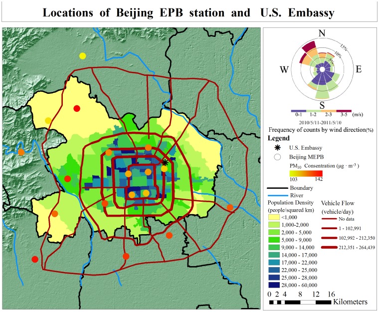
Daily PM10 concentration data were collected from May 10, 2010 to December 6, 2011 at the 18 authorized (BJ-EPB) observation stations, which are evenly distributed across the city. Daily PM2.5 concentrations reported by the embassy monitoring station were also gathered for the same period. Days with long periods of missing PM2.5 (hourly) data were discarded based on the following criterion: if during a day there were consecutive data gaps of more than 3 hours or the cumulative amount of missing data exceeded 12 hours, that day was not included in pollution estimation. The final result was a dataset covering a 423-day period. We also acquired information about the geographic locations of the U.S. Embassy and 18 BJ-EPB stations, as well as data on population density, main traffic routes, traffic flow volumes, daily mean wind direction and speed, and geomorphology. All data were stored in a Geographic Information System (GIS), and are represented in Figure 1.
Figure 1. Location of BJ-EPB PM10 monitoring stations and U.S Embassy PM2.5 station (Beijing, China).
The SPA Technique
We developed a technique, called Single Point Areal Estimation (SPA), which belongs to the category of biased areal estimation techniques [23]. SPA was used to extend the temporal PM2.5 data recorded at a single (U.S. Embassy) monitoring station to areal-average PM2.5 pollutant estimates, taking advantage of physical correlations between the PM2.5 mass concentrations (U.S. Embassy station) and the PM10 data (18-station BJ-EPB network). This point-to-area transformation yields best linear unbiased estimates (BLUE) of PM2.5 spatial averages over the entire city of Beijing. A formal derivation of the SPA technique is given in the following.
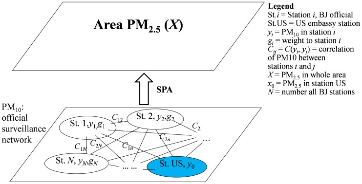
The objective of the SPA technique is to estimate citywide PM2.5 pollution in the Beijing area. The estimate is based on PM2.5 data from a single monitoring station at the U.S. Embassy in Beijing, and PM10 concentrations observations obtained at the official BJ-EPB monitoring network. Figure 2 outlines the SPA method.
Figure 2. Relationship between stations and PM2.5 areal concentration: yi denotes PM10 concentration reported by station i, and X is areal PM2.5 concentration for Beijing; St. US denotes the U.S. Embassy station at which daily PM2.5 concentration x0 is observed; X is estimated by x 0 using the SPA technique, based on observed PM2.5 data at the embassy station, and their correlation with PM10 concentrations observed at the 18 (evenly distributed) stations operated by BJ-EPB.
The true average PM2.5 concentration (X) over the entire area per time unit (e.g., daily) is calculated in theory by
| (1) |
where xi (i = 1, …, 18) denotes PM2.5 concentration at the i-th station (which, in the present study, was not available from the official surveillance network); N denotes the total number of observation stations (18 in this case); gi denotes the weight (contribution) of the i-th observation station to PM2.5 estimation so that  (unbiased estimation). There is only one PM2.5 monitoring station (U.S. Embassy). Accordingly, the areal PM2.5 concentration for Beijing is estimated by
| (2) |
where x0 denotes hourly PM2.5 concentration at the single monitoring station, as reported by the embassy and made available via the web site Twitter.com; w0 denotes the weight assigned to the embassy PM2.5 observation. This weight is estimated by minimizing
| (3) |
where vX is the variance of the estimated area-averaged X ( = PM2.5 concentration); and the E(·) denotes statistical mean.
At the same time, it is valid that
| (4) |
i.e., the SPA technique generates an unbiased pollutant estimate that is also the best (in the minimum mean squared estimation error sense).
Derivation of the SPA Equations
The variance of  is derived as
 |
(5) |
where C(·) is the covariance between concentrations at any pair of points (the covariance provides a quantitative assessment of the spatial dependence between concentrations at these points).
The first term in Eq. (5) is
| (6) |
the second term is
| (7) |
and the third item is
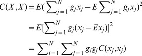 |
(8) |
By substituting Eqs. (6)–(8) into Eq. (5), we obtain
 |
(9) |
Taking into consideration the unbiased condition of Eq. (4), the Lagrange parameter μ is introduced into Eq. (9) in the following manner:
 |
(10) |
Minimization of Eq. (10) with respect to the  ’s,
’s,  and
and  is a standard optimization problem, leading to the system of equations (to be solved with respect to
  ,
,  ,
,  and
and  ):
):
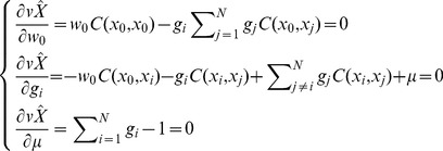 |
(11) |
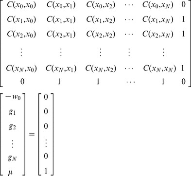
This system of equations can be written in matrix notation as
 |
(12) |
The solution of Eq. (12) yields w 0, gi and μ, as appropriate.
Accuracy of the SPA Technique
A variety of studies have discussed the uncertainty sources affecting the accuracy of data-based air quality estimates [24], [25]. Generally, there is an inverse relationship between uncertainty and accuracy – the higher the data uncertainty, the lower the accuracy of a model or technique. Usually the accuracy of a technique is measured in terms of its estimation error. The theoretical background of the SPA technique considers both horizontal correlations between samples, and vertical correlations between samples and area populations. It subsequently produces pollutant estimates that satisfy two key criteria – unbiasedness and minimum estimation error. Accordingly, SPA is a network-based estimation technique that is resistant to shifts [26] such as dust storms, which are addressed by statistical autocorrelation parameters in the model.
In this study, the horizontal (spatial) correlation between PM2.5 concentrations is approximated by that between spatial PM10 concentrations. The estimation error of this approximation is small due to various reasons:
The citywide PM2.5 concentration estimated by SPA is defined as the weighted spatial PM2.5 average from all 18 stations (for each station the weight was proportional to the associated Voronoi area). Note that spatial topology –which is a key determinant of horizontal (spatial) autocorrelation [27]– is identical for PM2.5 and PM10 [28].
Both particulates vary in space and time, subject to the same weather conditions, providing a valuable determinant of horizontal correlation [29], [30]. Vertical correlations between PM2.5 and PM10 concentrations were calibrated in terms of the observed data.
Empirical evidence has shown that PM2.5 and PM10 concentrations are highly correlated, with values as high as 0.85 and 0.97, respectively [31], [32].
In the SPA technique, the correlation coefficients between PM2.5 and PM10 are calibrated by the data so that they can correct for potential discrepancies (see section 2 in the SI text). Historical data have shown high correlations between the U.S. Embassy PM2.5 concentrations and the 18 PM10 observation stations (Table 1). The maximum and minimum values of Pearson correlation efficient are 0.85 and 0.69, respectively.
Table 1. Pearson correlation coefficient between the U.S. Embassy PM2.5 concentration and 18 Beijing EPB PM10 concentrations.
| BJ-EPB Station | r | BJ-EPB Station | r |
| Aotizhongxin | 0.81 | Longquanzhen | 0.82 |
| Changpingzhen | 0.72 | Nongzhanguan | 0.83 |
| Dongsi | 0.83 | Tiantan | 0.82 |
| Fengtaihuanyuan | 0.85 | Tongzhouzhen | 0.79 |
| Gucheng | 0.81 | Wanliu | 0.81 |
| Guanyuan | 0.83 | Wanshouxigong | 0.84 |
| Haidingbeibuxinqu | 0.69 | Yizhuangkaifaqu | 0.82 |
| Huangcunzhen | 0.80 | Yungang | 0.81 |
| Liangxiang | 0.82 | Zhiwuyuan | 0.77 |
Estimation precision was further assessed by a validation study using an exhaustive PM10 dataset in the study area. In particular, daily areal PM10 concentrations were estimated by the SPA technique based on records at each of the 18 PM10 stations. The actual daily areal PM10 concentration is the weighted spatial PM10 average from all 18 stations (for each station, the weight was proportional to the associated Voronoi area; see Supporting material). Subsequently, the areal PM10 concentration estimated by each of the 18 PM10 monitoring stations and SPA was compared to the actual concentration value, resulting in good agreement (Table 2 and Figure S1 in SI text). This result supports the reliability of the SPA technique when used to estimate areal pollution concentration based on a single monitoring station. An SPA software is provided that can be used to perform the data calculations of this study (www.sssampling.org/SPA). Readers can apply the SPA software to their own data.
Table 2. Summary of R2 values of the linear relationships between Beijing areal PM10 estimated on the basis of a single station using SPA and the true area.
| BJ-EPB Station | R2 | BJ-EPB Station | R2 |
| Aotizhongxin | 0.961 | Longquanzhen | 0.921 |
| Changpingzhen | 0.862 | Nongzhanguan | 0.966 |
| Dongsi | 0.969 | Tiantan | 0.941 |
| Fengtaihuanyuan | 0.961 | Tongzhouzhen | 0.867 |
| Gucheng | 0.933 | Wanliu | 0.947 |
| Guanyuan | 0.964 | Wanshouxigong | 0.971 |
| Haidingbeibuxinqu | 0.764 | Yizhuangkaifaqu | 0.888 |
| Huangcunzhen | 0.896 | Yungang | 0.925 |
| Liangxiang | 0.849 | Zhiwuyuan | 0.901 |
Results
Daily PM2.5 mass concentrations observed at the embassy station ranged from 4 to 487 µg/m3 for the 423-day period. The annual average concentration (December 7, 2010–December 6, 2011) was 98.85 µg/m3, with high temporal variability. For the entire time series, the highest PM2.5 concentrations (>300 µg/m3) occurred during 10 days: December 7 and November 18–19, 2010, February 21–24, October 23 and December 5, 2011; see Figure 3.
Figure 3. PM2.5 concentration observed by a single station (U.S. Embassy), and estimated citywide PM2.5 areal concentration (Beijing, China).
During the same period, estimated citywide PM2.5 daily pollution in Beijing ranged from 2.86 to 318.29 µg/m3. The annual average pollution was 64.78 µg/m3. The highest concentrations (>300 µg/m3) occurred during two days, November 19, 2010 and February 21, 2011, as shown in Figure 3.
Discussion
It was found that the U.S. Embassy PM2.5 observations exhibited approximately the same trend as citywide PM2.5 areal concentrations estimated by the SPA technique, although the embassy’s concentration values were clearly higher. The most important reason for this could be that the U.S. Embassy is at the city center, where population density and traffic volume are the highest in the city. The ratio between the embassy’s PM2.5 concentration and the estimated area-average concentration pollution varied with time. It is affected by the dynamic correlation between PM2.5 and PM10, caused by variation in local emission and atmospheric conditions between the embassy and the entire city.
Estimated area-average PM2.5 concentrations varied on a daily and monthly basis. The lowest concentrations occurred during January and March 2011, owing to the large number of windy days (refer to Figure S2 in SI text for monthly wind speeds). Estimation uncertainty is high for March 2011, because of serious data gaps. The highest concentrations occurred during July and November 2010, and during February and July–September 2011. During November, formation of a temperature inversion layer was observed over Beijing, which is a meteorological condition that plays an important role in the accumulation of PM2.5. The PM2.5 mass concentration peak during February was most likely due to emissions from coal consumption for heating purposes [33], [34]; this was the month with the lowest temperatures and slowest winds during 2011. July–September was the hottest period during a year. Long and intense solar irradiation during summer favors photochemical formation of aerosol particles [35], [36], which benefits the synthesis of PM2.5. This caused the high PM2.5 levels observed during that season. As regards seasonal variation, winter and summer had higher PM2.5 levels, with concentrations 68.74 µg/m3 and 70.42 µg/m3, respectively. Spring and fall concentrations were 63.59 µg/m3 and 61.54 µg/m3, respectively.
In sum, PM2.5 pollution in Beijing remained relatively high during the study period (Figure 3). Daily and annual interim target-1 standards recommended by the World Health Organization (WHO) are 75 µg/m3 and 35 µg/m3, respectively [37]. As mentioned earlier, the annual (December 7, 2010–December 6, 2011) average concentration in Beijing was 64.78 µg/m3. During that period, daily concentrations during 93 out of 259 days exceeded the WHO standard. Compared to the Beijing PM2.5 levels of five years ago reported in previous studies [33], [34], this level has dropped significantly. The situation may be attributed to a policy of prioritizing development of public transport, displacement of heavy industrial factories away from the city, and other efforts associated with the 2008 Beijing Olympics. Yet, the number of cars in the city has grown, from 2.6 million in 2005 to 5 million in 2010. Furthermore, air quality remains dependent on weather conditions, which means that considerable willingness and effort are needed to eliminate PM2.5 sources, thereby clearing the sky over the city.
Conclusion
PM air pollution is a severe problem for Beijing city, as is demonstrated by both the official PM10 and the estimated PM2.5 concentrations. The areal PM2.5 concentration estimated by the proposed SPA technique was found to be a little lower than that observed at the U.S. Embassy monitoring station that is located at the city center and near a traffic junction. Validation results showed that the SPA technique is a useful tool in the estimation of areal PM2.5 concentration, even when only one PM2.5 observation station is available. Concerning the in situ implementation of SPA, (i) the key input to the technique is the correlation (covariance) between the PM2.5 and PM10 stations calculated from historical data, (ii) the estimation weight of the PM2.5 station was obtained by solving a linear equation (equation (12)) and, subsequently, (iii) the areal PM2.5 concentration was calculated from equation (2). Concluding, given the prohibitive costs of measurement campaigns and monitoring networks, the proposed SPA technique can be an effective and accurate pollution estimation tool, especially in cases in which, due to limited monitoring stations or in remote areas or in the past, other sources of information need to be used.
Supporting Information
Details on data, estimation, the accuracy test, and a software of the method are available free of charge online at http://pubs.acs.org, or from www.sssampling.org/SPA.
Supporting Information
Data description & model validation.
(DOC)
Original data.
(XLS)
Funding Statement
This study was supported by the following grants: NSFC (41023010; 41271404), MOST (2012CB955503; 2011AA120305) and CAS (XDA05090102). George Christakos was supported by a Yongqian Chair Professorship (Zhejiang University, China). The funders had no role in study design, data collection and analysis, decision to publish, or preparation of the manuscript.
References
- 1. Bayraktar H, Turalioglu FS, Tuncel G (2010) Average mass concentrations of TSP, PM10 and PM2.5 in Erzurum urban atmosphere, Turkey. Stochastic Environmental Research and Risk Assessment 24: 57–65. [Google Scholar]
- 2. Wiwanitkit V (2008) PM10 in the atmosphere and incidence of respiratory illness in Chiangmai during the smoggy pollution. Stochastic Environmental Research and Risk Assessment 22: 437–440. [Google Scholar]
- 3. Kaiser J (2000) Air pollution - Evidence mounts that tiny particles can kill. Science 289: 22–23. [DOI] [PubMed] [Google Scholar]
- 4.Ostro B (2004) Outdoor Air Pollution: Assessing the Environmental Burden of Disease of Outdoor Air Pollution at National and Local Levels. Geneva: World Health Organization, (WHO Environmental Burden of Disease Series, No. 5).
- 5. Pyne S (2002) Air pollution - Small particles add up to big disease risk. Science 295: 1994–1994. [DOI] [PubMed] [Google Scholar]
- 6. Nel A (2005) Air pollution-related illness: Effects of particles. Science 308: 804–806. [DOI] [PubMed] [Google Scholar]
- 7. Akimoto H (2003) Global air quality and pollution. Science 302: 1716–1719. [DOI] [PubMed] [Google Scholar]
- 8. Lelieveld J, Berresheim H, Borrmann S, Crutzen PJ, Dentener FJ, et al. (2002) Global air pollution crossroads over the Mediterranean. Science 298: 794–799. [DOI] [PubMed] [Google Scholar]
- 9. Kaiser J (1997) Particulate matter - Getting a handle on air pollution’s tiny killers. Science 276: 33–33. [DOI] [PubMed] [Google Scholar]
- 10. Guzman F, Ruiz ME, Vega E (1996) Air quality in Mexico City. Science 271: 1040–1041. [DOI] [PubMed] [Google Scholar]
- 11. Fu BJ (2008) Blue skies for China. Science 321: 611–611. [DOI] [PubMed] [Google Scholar]
- 12. Marshall JD, Nethery E, Brauer M (2008) Within-urban variability in ambient air pollution: Comparison of estimation methods. Atmospheric Environment 42: 1359–1369. [Google Scholar]
- 13.US-Embassy-in-Beijing (2011) U.S Embassy Beijing Air Quality Monitor, Available at: http://eng.embassyusa.cn/070109air.html.
- 14.XinHuaNet (2011) Chinese and U.S. Experts Explain Beijing Air Quality Monitoring Data, Available at: http://news.xinhuanet.com/society/2011-11/08/c_111153803.htm.
- 15.BJ-EPB (2011) Beijing Municipal Environmental Protection Bureau Daily Air Quality, Available at: http://www.bjepb.gov.cn/air2008/Air.aspx.
- 16. MEP-PRC (1996) People’s Republic of China National Standard. Ambient air quality standard GB3095–1996: 2. [Google Scholar]
- 17. Brook JR, Dann TF, Burnett RT (1997) The relationship among TSP, PM(10), PM(2.5), and inorganic constituents of atmospheric particulate matter at multiple Canadian locations. Journal of the Air & Waste Management Association 47: 2–19. [Google Scholar]
- 18. Gomiscek B, Hauck H, Stopper S, Preining O (2004) Spatial and temporal variations Of PM1, PM2.5, PM10 and particle number concentration during the AUPHEP-project. Atmospheric Environment 38: 3917–3934. [Google Scholar]
- 19. Lundgren DA, Hlaing DN, Rich TA, Marple VA (1996) PM(10)/PM(2.5)/PM(1) data from a trichotomous sampler. Aerosol Science and Technology 25: 353–357. [Google Scholar]
- 20. Li CS, Lin CH (2002) PM1/PM2.5/PM10 characteristics in the urban atmosphere of Taipei. Aerosol Science and Technology 36: 469–473. [Google Scholar]
- 21. Maraziotis E, Sarotis L, Marazioti C, Marazioti P (2008) Statistical analysis of inhalable (PM10) and fine particles (PM2.5) concentrations in urban region of Patras, Greece. Global Nest Journal 10: 123–131. [Google Scholar]
- 22. van de Kassteele J, Koelemeijer RBA, Dekkers ALM, Schaap M, Homan CD, et al. (2006) Statistical mapping of PM10 concentrations over Western Europe using secondary information from dispersion modeling and MODIS satellite observations. Stochastic Environmental Research and Risk Assessment 21: 183–194. [Google Scholar]
- 23. Wang JF, Reis BY, Hu MG, Christakos G, Yang WZ, et al. (2011) Area Disease Estimation Based on Sentinel Hospital Records. PLoS ONE 6: 1–8. [DOI] [PMC free article] [PubMed] [Google Scholar]
- 24. Christakos G, Vyas VM (1998) A composite space/time approach to studying ozone distribution over Eastern United States. Atmospheric Environment 32: 2845–2857. [Google Scholar]
- 25. Jerrett M, Newbold KB, Burnett RT, Thurston G, Lall R, et al. (2007) Geographies of uncertainty in the health benefits of air quality improvements. Stochastic Environmental Research and Risk Assessment 21: 511–522. [Google Scholar]
- 26. Reis BY, Kohane IS, Mandl KD (2007) An epidemiological network model for disease outbreak detection. Plos Medicine 4: 1019–1031. [DOI] [PMC free article] [PubMed] [Google Scholar]
- 27.Isaaks EH, Srivastava RM (1989). Applied Geostatistics. New York: Oxford University Press.
- 28. Kumar N (2009) An optimal spatial sampling design for intra-urban population exposure assessment. Atmospheric Environment 43: 1153–1155. [DOI] [PMC free article] [PubMed] [Google Scholar]
- 29. Tiwari S, Chate DM, Pragya P, Ali K, Bisht DS (2012) Variations in Mass of the PM10, PM2.5 and PM1 during the Monsoon and the Winter at New Delhi. Aerosol and Air Quality Research 12: 20–29. [Google Scholar]
- 30. Pandey P, Khan AH, Verma AK, Singh KA, Mathur N, et al. (2012) Seasonal Trends of PM2.5 and PM10 in Ambient Air and Their Correlation in Ambient Air of Lucknow City, India. Bulletin of Environmental Contamination and Toxicology 88: 265–270. [DOI] [PubMed] [Google Scholar]
- 31. Kumar R, Joseph AE (2006) Air pollution concentrations of PM2.5, PM10 and NO2 at ambient and kerbsite and their correlation in Metro City - Mumbai. Environmental Monitoring and Assessment 119: 191–199. [DOI] [PubMed] [Google Scholar]
- 32. Marcazzan GM, Vaccaro S, Valli G, Vecchi R (2001) Characterisation of PM10 and PM2.5 particulate matter in the ambient air of Milan (Italy). Atmospheric Environment 35: 4639–4650. [Google Scholar]
- 33. Wang HL, Zhuang YH, Wang Y, Sun Y, Yuan H, et al. (2008) Long-term monitoring and source apportionment of PM(2.5)/PM(10) in Beijing, China. Journal of Environmental Sciences-China 20: 1323–1327. [DOI] [PubMed] [Google Scholar]
- 34. Zheng M, Salmon LG, Schauer JJ, Zeng L, Kiang CS, et al. (2005) Seasonal trends in PM2.5 source contributions in Beijing, China. Atmospheric Environment 39: 3967–3976. [Google Scholar]
- 35. Song Y, Tang XY, Xie SD, Zhang YH, Wei YJ, et al. (2007) Source apportionment of PM2.5 in Beijing in 2004. Journal of Hazardous Materials 146: 124–130. [DOI] [PubMed] [Google Scholar]
- 36. Wang Y, Zhuang GS, Tang AH, Yuan H, Sun YL, et al. (2005) The ion chemistry and the source of PM2.5 aerosol in Beijing. Atmospheric Environment 39: 3771–3784. [Google Scholar]
- 37.WHO-Europe (2006) Air Quality Guidelines, Global Update 2005: Particulate Matter, Ozone, Nitrogen Dioxide, and Sulfur Dioxide: World Health Organization Europe. 22 p. [PubMed]
Associated Data
This section collects any data citations, data availability statements, or supplementary materials included in this article.
Supplementary Materials
Data description & model validation.
(DOC)
Original data.
(XLS)


