Quantification of Transmembrane Currents during Action Potential Propagation in the Heart

Abstract

The measurement, quantitative analysis, theory, and mathematical modeling of transmembrane potential and currents have been an integral part of the field of electrophysiology since its inception. Biophysical modeling of action potential propagation begins with detailed ionic current models for a patch of membrane within a distributed cable model. Voltage-clamp techniques have revolutionized clinical electrophysiology via the characterization of the transmembrane current gating variables; however, this kinetic information alone is insufficient to accurately represent propagation. Other factors, including channel density, membrane area, surface/volume ratio, axial conductivities, etc., are also crucial determinants of transmembrane currents in multicellular tissue but are extremely difficult to measure. Here, we provide, to our knowledge, a novel analytical approach to compute transmembrane currents directly from experimental data, which involves high-temporal (200 kHz) recordings of intra- and extracellular potential with glass microelectrodes from the epicardial surface of isolated rabbit hearts during propagation. We show for the first time, to our knowledge, that during stable planar propagation the biphasic total transmembrane current (I_m) dipole density during depolarization was ∼0.25 ms in duration and asymmetric in amplitude (peak outward current was ∼95 μA/cm² and peak inward current was ∼140 μA/cm²), and the peak inward ionic current (I_ion) during depolarization was ∼260 μA/cm² with duration of ∼1.0 ms. Simulations of stable propagation using the ionic current versus transmembrane potential relationship fit from the experimental data reproduced these values better than traditional ionic models. During ventricular fibrillation, peak I_m was decreased by 50% and peak I_ion was decreased by 70%. Our results provide, to our knowledge, novel quantitative information that complements voltage- and patch-clamp data.

Introduction

The quantitative characterization of transmembrane potential (V_m) and transmembrane currents has been an integral part of the field of cardiac electrophysiology since its inception. The total transmembrane current (I_m) is the sum of a capacitive current (I_c) and a resistive current referred to as I_ion

$$I_m=I_c+I_{ion}.$$ (1)

The capacitance current acts to charge the membrane (excess charge accumulates at the lipid bilayer surfaces) and is represented as

$$I_c=C_m\frac{d{V}_m}{dt},$$ (2)

where C_m is membrane capacitance and t is time. I_ion is the sum of many ionic currents (primarily potassium, sodium, and calcium) flowing through channels in the membrane, V_m is equal to V_i – V_e where V_i is intracellular potential and V_e is extracellular potential. Most of the ionic currents are nonlinear functions of V_m and t; for example, the rapid sodium current (I_Na), which gives rise to fast membrane depolarization, is typically represented mathematically as

$$I_{Na}={\mathrm{g}}_{Na}\left(V_m-E_{Na}\right),$$ (3)

where g_Na is the sodium channel conductance, which is a function of both V_m and t, and E_Na is the Nernst equilibrium potential for sodium (1).

Voltage clamp (2) and patch clamp (3) methods involve controlling V_m via a feedback current (equal to I_m), which is then analyzed to determine the voltage and time dependence of ionic currents. Most clamp protocols involve switching between constant values of V_m in an effort to eliminate I_c such that the injected current is equal to I_ion. This feedback control approach has provided, to our knowledge, much new information regarding transmembrane ion currents (especially gating kinetics) and the effect of pharmaceuticals, but is restricted by several limitations. First, the experimental preparations and protocols used in voltage-clamp studies are not physiological and the experimental conditions may modify channel behavior (4). Second, the typical clamp waveforms are not the complex upstrokes of propagating action potentials (which result from a dynamic interplay of transmembrane and axial currents as described in the Supporting Material; see Fig. S1). Third, spatial homogeneity of V_m can be difficult to maintain and assess. Fourth, the resistance and capacitance of the glass microelectrode and the input impedance of the microelectrode electrometer limit the recording bandwidth and hence can affect the accuracy of the measurements of the most rapid transients in V_m. Most importantly, the current amplitudes and maximum conductance values in intact tissue depend on tissue parameters such as channel density, membrane area, surface/volume ratio, axial conductivities, etc., which are extremely difficult to measure. Therefore, although voltage-clamp results can be used to characterize the voltage and time dependence of membrane currents, computer simulations of conduction are employed to determine how these membrane dynamics are related to transmembrane current density and potentials during propagation in intact tissue. Although there are considerable experimental data regarding V_m that are used in the development and validation of numerical models of propagation, there is unfortunately a dearth of corresponding experimental data on the amplitude and shape of transmembrane currents during propagation in ventricular tissue. There are no formulas to predict propagation behavior (e.g., action potential shape, transmembrane currents, conduction velocity, etc.) directly from gating kinetic equations. Currents within intact tissue are particularly difficult to measure directly and are often computed from recordings of V_e gradients (5–7). During plane-wave propagation, which is effectively one-dimensional (1-D), I_m is also proportional to the spatial gradient of axial currents (and hence the second spatial derivative of potential):

$$I_m=C_m{D}_i\frac{{\partial }^2{V}_i}{\partial x^2}=-C_m{D}_e\frac{{\partial }^2{V}_e}{\partial x^2},$$ (4)

where D_i (D_e) is the intracellular (extracellular) diffusion coefficient in cm²/ms, and x is the direction of propagation. Equation 4 is derived based on first principles (Ohm’s law and the conservation of current). Inward I_m behind the wavefront is often called the driving source for action potential propagation and the outward I_m ahead of the wavefront is considered the load or sink opposing propagation (see Fig. S1).

In this work we present, to our knowledge, a novel methodology to experimentally quantify cardiac transmembrane currents from potential recordings during stable propagation in the intact heart and provide the first values of both I_m and I_ion during ventricular epicardial conduction. Our approach is unique from alternatives involving measurements of multiple extracellular/interstitial potentials acquired with fine spatial sampling resolution because we compute transmembrane currents from high temporal resolution measurements of intracellular potential at a single site using a coordinate transformation based on conduction velocity measurements. Numerical simulations of propagation using four different representations of I_Na were also carried out to allow comparison and insight into the characterization and interpretation of our experimental results. Finally, we provide, to our knowledge, a novel model of cardiac action potential propagation incorporating experimentally derived current-voltage relationships of both depolarization and repolarization containing no gating variables and only six parameters.

Methods

Overall approach

Here, we quantify I_m, I_ion, and I_c throughout the cardiac action potential during stable propagation on the surface of the isolated rabbit heart using high-speed (200 kHz) glass microelectrode recordings of V_i and V_e at one site. We follow the pioneering approach of Jenerick (8–12), who proposed a method to compute transmembrane currents from microelectrode recordings of 1-D striated skeletal muscle fibers using the cable equation (13) and converted spatial gradients to temporal gradients by assuming stable propagation. We compute I_m, I_ion, and I_c according to

$$I_{ion}=I_m-I_c=\frac{C_m{D}_i}{\mathit{C}{\mathit{V}}^2}\frac{d^2{V}_i}{d{t}^2}-C_m\frac{d{V}_m}{dt},$$ (5)

where CV is conduction speed in the direction of propagation. Equation 5 includes the second temporal derivative of V_i and thus maintains the bidomain representation (incorporating both intra- and extracellular regions) in comparison to the monodomain (cable) equation, which instead contains the second derivative of V_m (this is discussed in more detail below). To reduce the dimensionality of the problem, we initiated planar propagation either along (longitudinal) or across (transverse) fibers using multiple extracellular stimulation electrodes (2). Stable, and nearly planar, wave propagation was observed in all hearts as assessed by the optical mapping data. Fig. 1 shows example isochrone maps indicating the position of the wave front at multiple instants demonstrating stable (i.e., constant CV), nearly planar propagation in the longitudinal (panel A) and transverse (panel B) directions on the surface of the rabbit heart.

Figure 1.

Isochrone maps from an isolated rabbit heart indicating the position of the wavefront at 1 ms intervals for propagation in the longitudinal (A) and transverse (B) directions. Wave propagation was initiated just outside the field of view (indicated by an asterisk) and the position of the microelectrode is indicated by M. The isochrone maps show nearly planar propagation through this region because the isochrones are nearly straight and parallel to each other.

Experimental preparation

All experiments followed the guidelines of the National Institutes of Health for the ethical use of animals in research and were approved in advance by the Vanderbilt Institutional Animal Care and Use Committee. Optical data acquisition, external stimulation, and laser illumination were all controlled via custom software written in C. Six (n = 6) New Zealand white rabbits of either sex weighing at least 3 kg were preanesthetized with ketamine (50 mg/kg), and then heparinized (1000 units) and anesthetized by pentobarbital sodium injection (60 mg/kg) into an ear vein. After a midsternal incision, the heart was removed and mounted on a Langendorff apparatus for retrograde perfusion through the aorta with oxygenated (95% O₂/5% CO₂) modified Tyrode’s solution of the following composition (mM): 133 NaCl, 4 KCl, 2 CaCl₂, 1 MgCl₂, 1.5 NaH₂PO₄, 20 NaHCO₃, and 10 glucose. The excitation-contraction uncoupler diacetyl monoxime was added to the perfusate at a concentration of 15 mM (Invitrogen, Carlsbad, CA) to eliminate contractile artifacts in the optical recordings. The temperature and pH were maintained at 37^°C and 7.4, respectively, and coronary perfusion pressure was 50 mmHg. To stain the heart with a voltage-sensitive dye, 200 μL of di-4-ANEPPS (Molecular Probes, Eugene, OR) of stock solution (0.5 mg/mL dimethyl sulfoxide) was administrated via an injection port above the aorta. A global electrocardiogram signal was continuously monitored (and saved for all episodes) with an oscilloscope (Tektronix, TDS5000B, Richardson, TX) using two Ag-AgCl pellet electrodes (EP8; World Precision Instruments, Sarasota, FL) placed on opposite sides of the heart. One additional heart was sacrificed to study ventricular fibrillation (VF) as described below.

Microelectrode recordings

To measure intra- and extracellular potentials, floating 3-M KCl-filled microelectrodes were used. The microelectrodes were pulled from borosilicate glass capillaries (World Precision Instruments) by a micropipette puller (Model P80/PC, Sutter Instrument, Novato, CA). The microelectrode tips were mounted on 50-μm-diameter platinum wire. The Ag/AgCl reference electrode, 8 mm in diameter and 1 mm in thickness (EP8; World Precision Instruments) was placed in the left ventricular cavity. To measure intra- and extracellular potentials from the same site, the microelectrode was gently pulled out from the cell after completion of the V_i recording and thereafter the sequential recording of V_e from the same approximate location was measured. Repeatability of the activation sequence was ensured by the superposition of the two electrocardiograms. The microelectrode and reference outputs were connected to the input probes of a dual differential electrometer (Model FD223, World Precision Instruments) with a response time of 0.5 μs. The signals were digitized, and recorded on a digital oscilloscope (Tektronix, TDS5000B). Microelectrode data were digitized at 200 kHz and then Gaussian filtered with a width of 0.055 ms (11 points), downsampled and then saved at 20 kHz for analysis. The frequency response of this Gaussian filter exhibits a half-decay frequency of 21 kHz with no ringing. Thirty-two beats were averaged to improve signal quality. This approach satisfies the most stringent requirement of 15 kHz proposed for recordings from Purkinje fibers (14). The effect of sampling rate on our results is provided in the Supporting Material. Recordings from one impalement within the field of view of the optical recordings from each heart were analyzed. Derivatives were computed using a two-point central difference. Because the I_m waveform was indistinguishable from noise during repolarization, the peak outward ionic current $\left(I_{ion}^{\mathit{max}}\right)$ was computed as the maximum value of the time derivative of −V_m computed using 15 data points (0.75 ms) via the Savitzky-Golay smoothing method using a second order local polynomial regression around each point (see horizontal arrow in Fig. 2 D). For VF, all derivatives were computed using 5 data points using second order polynomial fitting (Savitzky-Golay smoothing).

Figure 2.

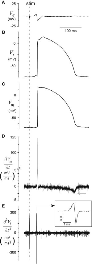
Microelectrode data. (A) V_e and (B) V_i recordings, (C) V_m signal computed as difference of V_i and V_e, (D) the first derivative of the V_m, and (D) the second derivative of the V_i signal from a glass microelectrode.

Waveform characterization

In this work, we use the traditional approach of representing transmembrane currents as current density per unit membrane surface area, in units of microamps per cm² (μA/cm²). We computed the minima and maxima values of I_ion, I_c, and I_m and the duration of the biphasic I_m dipole during depolarization $\left(I_m^{dur}\right)$ as the time interval between $I_m^{\mathit{min}}$ and $I_m^{\mathit{max}}$; the duration of inward ionic current $\left(I_{ion}^{dur}\right)$ was computed as the width of the deflection containing 90% of the peak amplitude. Charge was computed by integrating the current waveforms, and the integration time was chosen to be 4 ms centered on the zero crossing of I_m (for VF, the integration time was chosen to be 6 ms).

Optical recordings

All recordings were from the epicardial surface of the anterior left ventricle. The voltage-sensitive dye di-4-ANEPPS was excited by a diode-pumped, solid-state laser (Verdi, Coherent, Santa Clara, CA) at a wavelength of 532 nm. The fluorescence emitted from the imaged area of the heart was collected by a 52-mm lens (Tiffen, Hauppauge, NY) and passed through a longpass filter (no. 25 Red, 607 nm, Tiffen). Images from an ∼1 cm × 1 cm region from the surface of the rabbit heart (average region size from all six hearts was 1.26 ± 0.05 cm²) were recorded at 40 × 40 pixels at 3 kHz via a 14-bit quad charge-coupled device camera (CardioCCD-SMQ, RedShirtImaging, Decatur, GA). One hundred beats were averaged to improve signal quality. The fluorescence action potential amplitude at each site was normalized and the activation time at each site was determined as the time the fluorescence increased past 50% using linear interpolation between frames (15).

Planar propagation was initiated both along (longitudinal) and across (transverse) fibers using multiple extracellular stimulation electrodes (16), and intracellular potentials for each heart were recorded from the same impalement followed by extracellular recordings while repeating the same pacing protocol. Propagation was initiated via low strength (∼1.5 × threshold) stimulation just outside the imaging region at a cycle length of 300 ms. Stable, and nearly planar, wave propagation was observed in all hearts as assessed by the optical mapping data and CV was computed from isochrone maps (15) at the site of microelectrode impalement as identified visually (see Fig. 1). The value of D_i in Eq. 5 was divided by the square of the anisotropy ratio (AR²) for transverse propagation computations where AR (2.45 ± 0.15) was the anisotropic ratio computed from the ratio of CVs resulting from elliptical wave propagation (see Fig. S2) (17). We assume constant values for C_m (1 μF/cm²) and D_i (0.001 cm²/ms) in the direction of fibers. The uncertainty of the values of C_m and D_i is discussed below.

Statistics

Values are presented as mean ± standard error. Statistical analysis was performed using paired two-tailed t-tests or one-tailed t-tests as appropriate.

Results

In this work, we present, to our knowledge, the first experimental quantification of the three components of the transmembrane current during planar wave propagation. Accordingly, we address the issues of signal quality and sampling rate as well as uncertainty in the values of C_m and D_i (see Table S1 and Table S2 and Figs. S3–S6). We perform simulations of wave propagation for three ionic models with different I_Na kinetics and compare them to our experimental results. Because none of these ionic models represented the time shape of the experimental transmembrane currents, we performed simulations based on our experimentally derived current-voltage relationships. Finally, to show feasibility of our approach we estimate transmembrane currents during VF.

Experimental transmembrane current quantification during pacing

The average CV for planar propagation computed at the site of the microelectrode impalement from all hearts was 59 ± 3 cm/s along fibers (longitudinal propagation, LP) and 32 ± 3 cm/s across fibers (transverse propagation, TP) (p < 0.001; n = 6). The average action potential amplitude (APA) of V_m was 109 ± 5 mV for LP and 112 ± 2 mV for TP (p = 0.5). An example of the sequential microelectrode recordings of V_e and V_i from one site during LP is shown in Fig. 2, A and B. The corresponding V_m trace, which is computed, is shown in Fig. 2 C. The derivatives computed from the V_m and V_i signals used to compute I_c and I_m (see Eq. 5) are shown in Fig. 2, D and E: I_c is proportional to the first derivative of V_m (see Eq. 2) and I_m is proportional to the second derivative of V_i, as shown in Eq. 5.

The waveforms of I_c, I_m, and I_ion during depolarization (only) are all shown in Fig. 3 A and follow the expected time course predicted by simulations (18). I_c first increases due to charging of the membrane during the foot of the V_m upstroke of the action potential. I_m first increases following I_c, whereas I_ion remains near zero and then becomes negative as the inward sodium current acts to depolarize the membrane. The maximal (positive) I_c $\left(I_c^{\mathit{max}}\right)$ and the minimal (negative) I_ion $\left(I_{ion}^{\mathit{max}}\right)$ occur during depolarization (i.e., at the wavefront). During depolarization, the fast sodium current is known to dominate I_ion and hence we quantified g_Na during propagation computed from the I_ion(t) and V_m data using Eq. 3 (assuming E_Na = V_m,rest + 130 mV); the average value of the maximal g_Na was 5.0 ± 1.0 mS/cm² for LP and 5.1 ± 1.0 mS/cm² for TP (p = 0.9). We also quantified the current-voltage relationship during the upstroke by plotting I_ion during depolarization versus normalized transmembrane potential ($V_m^{\ast }$), where $V_m^{\ast }$ (t) = V_m(t) – V_rest and normalized to the average APA of all animals (see Fig. 3 B). We show the individual curves for each animal as solid lines and the mean data across animals grouped into 5 mV bins are shown as symbols.

Figure 3.

Experimental transmembrane currents during pacing (depolarization only). (A) Current density (I_c, I_m, and I_ion) signals during depolarization (wavefront). (B) The current-voltage relationship, I_ion versus $V_m^{\ast }$ during depolarization, where $V_m^{\ast }$ = V_m – V_rest normalized to the averaged APA of all animals. The mean and standard errors of all animals are presented as symbols ($V_m^{\ast }$ grouped into 5 mV bins), whereas the individual curves of each animal are shown as solid lines.

The extreme values of I_c, I_m, and I_ion during depolarization were not statistically different between LP and TP, as shown in Fig. 4 A. For both directions of propagation, the magnitude of the peak inward I_m was greater than the outward peak I_m (p < 0.05), hence the waveform of I_m during depolarization was not symmetric with a larger inward peak current. The maximum value of I_m during repolarization (data not shown) was 2.8 ± 0.2 μA/cm² for LP and 3.0 ± 0.3 μA/cm² for TP (p = 0.2). During depolarization, averages of the charge densities on the membrane, Q_c, Q_m, and Q_ion, associated with each of the currents were not dependent on the direction of propagation, as shown in Fig. 4 B. During depolarization, inward and outward charge Q_m for both directions of propagation were not statistically different, unlike for peak I_m. Consistent with previous investigators (10,11), we found a significant (p = 0.001) linear correlation between $I_{ion}^{\mathit{min}}$ and $I_c^{\mathit{max}}$ slope = −0.48; intercept = 41.8).

Figure 4.

Peak values of experimental transmembrane current and charge densities during pacing (depolarization only). Average values and standard errors for all animals (n = 6) for both LP and TP are presented. (A) Current density (I_c, I_m, and I_ion) during depolarization. The peak inward phase of I_m was statistically different than the peak outward phase, as indicated by asterisks for both LP and TP. (B) Charge density (Q_c, Q_m, and Q_ion) during depolarization.

The time interval between the peak outward and inward I_m during depolarization (i.e., $I_m^{dur}$) was 0.27 ± 0.01 ms for LP and 0.25 ± 0.03 ms for TP (p = 0.3). Peak inward I_ion (i.e., $I_{ion}^{\mathit{min}}$) occurred during depolarization and its duration (i.e., $I_{ion}^{dur}$ was just over 1 ms (1.16 ± 0.3 ms for LP and 1.18 ± 0.1 ms for TP, p=0.9). The magnitude of peak I_c was not equal to the magnitude of peak I_ion (p < 0.05) nor were these peaks coincident; minimum I_ion occurred 0.14 ± 0.01 ms (0.1 ± 0.02 ms) later than peak I_c for LP (TP), p < 0.05, one-tailed t-test of difference for both LP and TP.

Bidomain versus monodomain representation

We used the bidomain representation of the cable equation, hence we computed I_c using V_m (see Eq. 2) but I_m using V_i (see Eq. 5). To assess whether the monodomain cable equation is appropriate for this study (planar epicardial propagation), we recomputed I_m using the second derivative of V_m (instead of the second derivative of V_i). The comparison of the I_m waveforms during depolarization (average from all animals, time aligned to maximum of I_c) is shown in Fig. S7 A. The two curves are basically superimposable, suggesting that either approach is justified. Experimentally, using microelectrodes, it would be easiest to apply the monodomain cable equation using only V_i. Therefore, we recomputed I_c using the first derivative of V_i (instead of the first derivative of V_m). The comparison of the I_c waveforms during depolarization is shown in Fig. S7 B. The two curves are also superimposable, suggesting that for the results presented here, using only intracellular data to compute transmembrane currents is justified.

Numerical simulations using ionic models

In our simulations using the three ionic models (BR, BRDR, and LRd) (19–21), the CV for action potential propagation ranged from 47 to 64 cm/s. We chose these three models because they incorporate different representations of I_Na, (see Eq. 3) and we only simulated the depolarization process. The time course of all transmembrane currents (I_c, I_ion, and I_m) exhibited the expected shapes (18); I_c was monophasic and positive, I_ion was monophasic and negative, and I_m was biphasic. The depolarization simulation results are provided for all three models in Table 1 (BR: g_Na,max = 4.0 and E_Na = 50; BRDR: g_Na,max = 15.0 and E_Na = 40; LRd: g_Na,max = 16.0 and E_Na = 55). The amplitude and duration of I_c, I_ion, and I_m during depolarization were model-dependent and could not be predicted a priori from the model parameters. I_m was biphasic, but not symmetric with a larger negative phase. The values computed for $I_{ion}^{\mathit{min}}$ (during depolarization) varied <2% compared to peak inward I_Na (a more detailed comparison is provided in Fig. S8).

Table 1.

Results of simulations of 1-D propagation (C_m = 1 μF/cm²; D_i = 1 cm²/s), using previously published BR, BDR, and LRd ionic models and our new parameterization f_d (V)

	BR	BRDR	LRd	fd (Vm)	LP	TP
CV (cm/s)	47	64	62.2	53	59	32
$I_c^{\mathit{max}}$(μA/cm2)	105	317	207	164	139	177
$I_m^{\mathit{max}}$(μA/cm2)	67.7	178	130	92	102	89
$I_m^{\mathit{min}}$(μA/cm2)	−75.5	−237	−226	−141	−159	−119
$I_m^{dur}$(ms)	0.39	0.20	0.26	0.26	0.27	0.25
$I_{ion}^{\mathit{min}}$(μA/cm2)	−146	−458	−360	−265	−263	−252
$I_{ion}^{dur}$(ms)	1.8	0.78	0.66	1.36	1.16	1.18
gNamax-1D	2.35	11.0	5.98	2.0	5.0	5.1

LP = longitudinal propagation; TP = transverse propagation.

Novel experimentally derived current-voltage relationships and corresponding simulations

Analytical relationships for I_ion as a function of $V_m^{\ast }$ during propagation were found separately for depolarization and repolarization by means of a symbolic regression algorithm Eureqa (http://creativemachines.cornell.edu/eureqa_download) (22). Symbolic regression was used to identify equations and initial parameters which were adjusted manually as described here.

For depolarization, the I_ion curves for LP for all six animals (see Figs. 3 B) were used as input to Eureqa. The resulting function f_d is our empirically derived ionic current versus voltage relationship for depolarization:

$$f_d\left(V\right)=a_{1}V-\frac{V}{a_2+a_{3}V+a_4{V}^2}.$$ (6)

This function contains only four parameters (compared to 25 for LRd I_Na). The original parameters’ values a₁ and a₂ were changed slightly (0.5% and 1%, respectively) to ensure the appropriate membrane resistance at rest (V = 0) (24). Parameters a₃ and a₄ were altered 0.2% and 0.1%, respectively, during the cable simulations to match the value of $I_{ion}^{\mathit{min}}$. The values of the parameters are a₁ = 0.55; a₂ = 4.0; a₃ = −0.1112; a₄ = 0.00082.

The analytical current-voltage relationship, function f_r, for I_ion during repolarization was found by inputting −$\text{d}{V}_m^{\ast }/\text{d}\mathit{t}$ as a function of $V_m^{\ast }$ for repolarization (only) for LP for all six animals (see Fig. 5 A) to Eureqa. The resulting current versus voltage relationship for repolarization was

$$f_r\left(V\right)=b_{1}V\exp \left(-b_{2}V\right).$$ (7)

Although the form of this function was determined by Eureqa, unlike depolarization, parameter values were adjusted significantly. Parameter b₁ was set to match membrane resistance at rest (24) and b₂ was changed by 18% to visually reproduce I_ion at high membrane potentials (see Fig. 5 A); final parameters values are: b₁ = 0.30; b₂ = 0.047.

Figure 5.

Novel, to our knowledge, current-voltage relationship and corresponding simulation results (repolarization). (A) I_ion during repolarization for all six animals (gray symbols) with our novel characterization (i.e., Eq. 7) superimposed as a thick black line. (B) $V_m^{\ast }$ for all six animals (thin gray lines) with a simulated action potential during propagation using our empirical characterization of I_ion (see Eq. 6–8) superimposed as a thick black line.

These two functions, Eqs. 6 and 7, were used to simulate propagation using the following equation

$$C_m\frac{\partial V}{\partial t}=C_m{D}_i\frac{{\partial }^{2}V}{\partial x^2}-f_{dr}\left(V\right),$$ (8)

where the function f_dr is equal to f_d for ∂V/∂t ≥ 0 and f_r for ∂V/∂t < 0. This equation is our cable equation, valid for both depolarization and repolarization, which includes our empirically derived current-voltage relationship. The resulting simulated action potential is shown as the dark curve in Fig. 5 B, which also shows recordings of the propagating action potentials from all six hearts. The equation reproduces well the shape and time course of the experimental data. $I_{ion}^{\mathit{max}}$ during repolarization for the simulated action potential was 2.4 μA/cm², which compares favorably to the experimental values of 2.8 for LP and 3.0 for TP. The time courses of all three transmembrane currents during depolarization for the simulated action potential are shown in Fig. 6, along with the average data and errors from the experimental data (all time-aligned to $I_c^{\mathit{max}}$ vertical dashed line). The corresponding transmembrane current waveforms reproduced the time course of the experimental data during the upstroke extremely well and much better compared to the BR, BRDR, and LRd models, as shown in Table 1.

Figure 6.

Simulations of propagation using our novel, to our knowledge, current-voltage relationships and correspondence to experimental data (depolarization only). The time course of the action potential upstroke (A) I_m (B), and I_ion (C) for our numerical simulations (thin black lines) using the experimentally derived I_ion(V) relationship presented in Eq. 6 along with experimental data for LP (symbols represent average and standard error of all six hearts). All data have been aligned to the time of $I_c^{\mathit{max}}$ indicated by a vertical dashed line.

Transmembrane current quantification during VF

A five-second episode of VF was recorded with both the charge-coupled device camera and a simultaneous recording of V_i from a glass microelectrode. Activation times were computed from both microelectrode and optical recordings and were consistent with a mean difference of 1.3 ms. Forty-five beats were identified from the optical recording, from which we categorized 27 as having stable epicardial propagation at the site of the microelectrode. The average CV magnitude for all 27 beats was 28 ± 3 cm/s (AR = 1.8 for this heart). A one second recording of V_i, the waveforms of I_c, I_m, and I_ion during depolarization (only), and activation sequences are shown for two beats during VF in Fig. 7. The average extreme values of I_c, I_m, and I_ion during depolarization during VF are shown in Fig. 8 A; the magnitude of the peak inward I_m was greater than the outward peak I_m (p < 0.05), hence the biphasic waveform of I_m during depolarization during VF was not symmetric with a larger inward peak current. During depolarization, the average values of the charge densities on the membrane, Q_c, Q_m, and Q_ion, associated with each of the currents during VF are shown in Fig. 8 B. Similar to planar propagation, there was a significant (p < 0.05) linear correlation between $I_{ion}^{\mathit{min}}$ and $I_c^{\mathit{max}}$ slope = −2.0; intercept = −0.1). $I_m^{dur}$ was increased 40% and the time difference between minimum I_ion and peak I_c was increased 90% compared to planar propagation.

Figure 7.

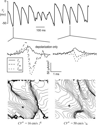
Transmembrane currents during experimental VF. (Top) One second recording of V_i from a microelectrode on the surface of the rabbit heart during VF. (Middle) Transmembrane currents during depolarization corresponding to these two beats. (Bottom) Isochrone maps of two beats (2 ms spacing).

Figure 8.

Peak values of experimental transmembrane current and charge densities during VF (depolarization only). Average values and standard errors for all animals (n = 6) are presented. (A) Current density (I_c, I_m, and I_ion) during depolarization. The peak inward phase of I_m was statistically different than peak outward phase, as indicated by asterisks. (B) Charge density (Q_c, Q_m, and Q_ion) during depolarization.

Discussion

The results presented here are relevant to all aspects of the relationship between membrane currents and potential as studied in basic electrophysiology experiments, simulations, and theory, which have been tightly intertwined since the pioneering work of Hodgkin and Huxley (1). Here, we present the implications of our work for these three complementary facets of electrophysiology.

Experiments

Our results include, to our knowledge, the first experimental quantitative characterization of the waveforms of all three cardiac transmembrane currents (I_m, I_ion, and I_c) during planar propagation in intact ventricular tissue. Our measurements of I_m using glass microelectrodes are qualitatively similar to the few previous experimental estimates obtained from ventricular cardiac tissue using extracellular arrays to measure V_e, but quantitatively different. Unlike the estimation of I_m using V_e as previous investigators (6,7,25), we compute I_m using the gold standard for V_m (microelectrodes) that provides a measurement of actual values of potential and hence transmembrane currents via a spatiotemporal coordinate transformation.

In contrast to previous results (6,25), we found that the biphasic waveform of I_m during normal depolarization was not symmetric but there was a larger inward peak current, although the corresponding charge delivered by each phase was the same. Implications of this asymmetry are discussed in the Supporting Material (see Fig. S9) as well in the Theory section below. As far as we know, there is only one study that reported the magnitude of I_m; Coronel et al. estimated the magnitude of peak I_m to be ∼35 μA/mm³ (6), which is 7.6 μA/cm² if we assume a surface/volume ratio of 4600 cm⁻¹ (26). This is an order of magnitude smaller than our estimate. We believe this difference can be explained by their electrode spacing (300 μm). We computed the duration of the biphasic I_m during depolarization to be 0.27 ms, which is shorter than the 0.44 ms computed (during sinus rhythm) by Witkowski et al. (25). We can compute the width of the I_m dipole as $I_m^{dur}$ ^∗CV, which equals 159 μm (LP) and 86 μm (TP). Therefore, as Wiley et al. (7) suggest, electrode spacing of <75 μm is required to accurately compute I_m from spatial gradients of potential. Our results indicate that a temporal sampling of ∼20 kHz is required to compute I_m accurately using our approach (see Fig. S4); the corresponding electrode spacing for spatial sampling is 30 μm (LP) and 16 μm (TP). Hence, the increased magnitude of I_m in our results compared to that of Coronel et al. (6) most likely reflects our use of high temporal sampling, which corresponds to an order of magnitude higher effective spatial sampling compared to Coronel et al. (6) In addition, considering that our value of peak I_m is an order of magnitude larger than the one previous estimate (6), our uncertainty of 60% (see the Supporting Material) for I_m is tolerable, albeit larger. As far as we know, there are no published values of measurements of I_ion during propagation in ventricular tissue.

Although the membrane kinetics of a plethora of ion channels have been extensively characterized, almost nothing is known about how the multiplicity of channels function together and affect the dynamics of propagation in tissue. Our experimental approach is a first step in quantifying and understanding the complex process of wave propagation through the heart resulting from the interplay of transmembrane and axial currents and potentials. It is important to note that, unlike most voltage-clamp studies in which I_ion(t) = −I_c(t), during propagation I_ion ≠ −I_c (because I_m ≠ 0, see Eq. 1 and Eq. 4). Our results show that the magnitude of I_ion is larger than (and not coincident with) I_c. It is well known that (∂V_m/∂t)_max of the action potential upstroke, which is thought to be a reflection of peak inward I_Na, is less during propagation compared to the single cell because of the loading imposed by the fact that cells are imbedded within a tissue with axial resistance. For example, (∂V_m/∂t)_max for isolated rabbit cells is over 400 mV/ms (27), which is more than twice the value we measured during propagation.

Computer simulations

Detailed ionic cellular models have been developed based on specific gating kinetics derived from voltage- and patch-clamp studies. These models are routinely used to study propagation in cardiac tissue and the model parameters (primarily gNa_max but also axial resistivity and surface/volume ratio) are adjusted to match the desired value of CV. These models cannot be expected to reproduce the specific details of propagation because no data from propagation were included in the development and validation of these models. We suggest that a more rigorous approach is required to develop models of propagation and our experimental results contain information to guide the development, modification, and validation of multicellular electrophysiological models. In contrast to detailed ionic models, models of reduced complexity allow unique insight via a bridge with theoretical approaches (24,28). Our simulations of propagation using our experimentally derived current-voltage relationships (Eq. 6–8) contain only six parameters and reproduce the time course of transmembrane currents better than the traditional representations of I_Na (see Table 1). We believe that this represents a fundamentally new approach in computational modeling. Traditionally, investigators fit experimental data to equations determined a priori, and the choice of these functions is often empirical. Here, a symbolic regression algorithm (Eureqa) (22) was used to identify the equations for the I-V relationship during depolarization (Eq. 6), and repolarization (Eq. 7). Both Eq. 6 and Eq. 7 are well behaved in that they do not give rise to spurious oscillations like generic polynomials. The I-V curve for repolarization, (f_r) with only two parameters, is similar to the time-independent potassium current (I_K1), which dominates during rapid repolarization (phase 3) that contains 10 or more parameters in traditional ionic models.

Theory

Theoretical analysis of the cable equation over the past 50 years has improved our understanding of wave propagation. This work provides significant insight into the relationship of the nonlinear I-V curve and propagation characteristics such as CV and the wavefront shape. CV and the exact shape of the propagating upstroke are interrelated and depend on the complex interdependence of axial and transmembrane current pathways as shown in Fig. S1. One advantage of theoretical studies is that analytical descriptions relating CV and wavefront shape to I-V can be formulated in certain situations. One of the restrictions for analytical predictions is that the shape of the wavefront (hence I_m) is symmetric (29,30). Our results suggest that theoretical work on how wavefront asymmetry affects wave propagation is of paramount importance in cardiac electrophysiology. Although cubic and quintic functions for f_d can be used to determine CV analytically (29), we found that these functions did not represent the data as well as our empirically derived Eq. 6. Although, to our knowledge, our novel model represents the complete action potential shape during propagation, threshold, the membrane resistance at rest, and during the plateau, it does not contain any gating variables and thus will not exhibit action potential duration or CV restitution. Adding one or more gating variables could rectify this limitation and still maintain analytical tractability similar to the Fitzhugh approach (31).

Limitations

Consistent with similar previous studies (5,8,9,11,32), all the results in this study are based on the assumption of stable propagation in which the spread of electrical activity through the three-dimensional heart is effectively reduced to a 1-D problem by assuming no dependencies in the directions perpendicular to the direction of propagation. This assumption is accurate (and bidomain is equivalent to the monodomain) as long as propagation is planar and either parallel or perpendicular to the fiber direction (33). Our data in Fig. S7 show that both I_m and I_c are the same whether they are computed from V_i or V_m, supporting our assumption of planar propagation. We neglected transmural effects, but we estimated this contribution to be <5% (see in the Supporting Material Eqs. S3–S5, and Fig. S10). The effect of curvature could be included analytically, with caution regarding high curvature and anisotropy, via Eqs. 4 and 5 (34–36). The values of C_m and D_i in cardiac tissue are extraordinarily difficult to measure and quantify. Therefore, as is common in the field of cardiac electrophysiology, we assumed constant values for C_m and D_i in ventricular epicardial tissue, even though there are considerable differences of C_m among cell types and significant variability of the reported values for D_i (37). We discuss the uncertainty within our data and the parameters C_m and D_i in regard to our results in the Supporting Material; a much more complicated issue is the true sources of experimental measurement variability. Here, we assume that C_m is constant (see Eq. 2) and hence our experimental variability of I_c is comparable to (dV_m/dt)_max in previous studies (38). However, the more fundamental issue is the relative contribution of the true underlying variability (animal-to-animal, spatial, temporal, etc.) of physiological parameters (e.g., C_m, axial conductivities, surface/volume ratio, etc.) to the experimental measurement variability of our transmembrane currents. The use of diacetyl monoxime may affect transmembrane current values, although our CV values compare favorably to those for epicardial propagation on the surface of the rabbit heart in control (39) and with 15 mM diacetyl monoxime (40). Our approach should allow for the separation of I_ion into its species components using pharmacological interventions to selectively block specific ion currents, but only if these interventions allow stable propagation.

Conclusions

In this work we present 1), the first, to our knowledge, experimental quantitative characterization of the waveforms of all three cardiac transmembrane currents (I_m, I_ion, and I_c) during planar propagation; and 2), a numerical model derived from the experimental data that reproduces these waveforms better than traditional ionic models. These results provide previously unavailable information that can be used to develop, modify, and validate mathematical models of propagation in cardiac tissue. Our work provides the experimental and theoretical basis to tease apart the dynamic interplay of I_m, I_ion, and I_c during stable propagation and provides quantitative insight into the relative roles and interdependence of active membrane dynamics and passive axial resistance. We demonstrate the feasibility of our approach by showing estimates of transmembrane currents during VF. We suggest that our approach provides similar and complementary data to voltage- and patch-clamp methodologies; thus, the quantification of the effects of pharmaceuticals on transmembrane currents using our approach is envisioned. In addition, the potential applicability of our approach and the accompanying insight to transmural propagation in the wedge preparation (41) is intriguing.

References

- 1.Hodgkin A.L., Huxley A.F. A quantitative description of membrane current and its application to conduction and excitation in nerve. J. Physiol. 1952;117:500–544. doi: 10.1113/jphysiol.1952.sp004764. [DOI] [PMC free article] [PubMed] [Google Scholar]
- 2.Cole K.S., Curtis H.J. Electric impedance of the squid giant axon during activity. J. Gen. Physiol. 1939;22:649–670. doi: 10.1085/jgp.22.5.649. [DOI] [PMC free article] [PubMed] [Google Scholar]
- 3.Neher E., Sakmann B. Single-channel currents recorded from membrane of denervated frog muscle fibres. Nature. 1976;260:799–802. doi: 10.1038/260799a0. [DOI] [PubMed] [Google Scholar]
- 4.Cachelin A.B., de Peyer J.E., Kokubun S., Reuter H. Sodium channels in cultured cardiac cells. J. Physiol. 1983;340:389–401. doi: 10.1113/jphysiol.1983.sp014768. [DOI] [PMC free article] [PubMed] [Google Scholar]
- 5.Witkowski F.X., Kavanagh K.M., Plonsey R. In vivo estimation of cardiac transmembrane current. Circ. Res. 1993;72:424–439. doi: 10.1161/01.res.72.2.424. [DOI] [PubMed] [Google Scholar]
- 6.Coronel R., Wilms-Schopman F.J., de Bakker J.M. Laplacian electrograms and the interpretation of complex ventricular activation patterns during ventricular fibrillation. J. Cardiovasc. Electrophysiol. 2000;11:1119–1128. doi: 10.1111/j.1540-8167.2000.tb01758.x. [DOI] [PubMed] [Google Scholar]
- 7.Wiley J.J., Ideker R.E., Pollard A.E. Measuring surface potential components necessary for transmembrane current computation using microfabricated arrays. Am. J. Physiol. Heart Circ. Physiol. 2005;289:H2468–H2477. doi: 10.1152/ajpheart.00570.2005. [DOI] [PubMed] [Google Scholar]
- 8.Jenerick H. Phase plane trajectories of the muscle spike potential. Biophys. J. 1963;3:363–377. doi: 10.1016/s0006-3495(63)86827-7. [DOI] [PMC free article] [PubMed] [Google Scholar]
- 9.Jenerick H. An analysis of the striated muscle fiber action current. Biophys. J. 1964;4:77–91. doi: 10.1016/s0006-3495(64)86770-9. [DOI] [PMC free article] [PubMed] [Google Scholar]
- 10.Freeman S.E., Turner R.J. The effects of l-propranolol and practolol on atrial and nodal transmembrane potentials. J. Pharmacol. Exp. Ther. 1975;195:133–139. [PubMed] [Google Scholar]
- 11.Freeman S.E., Leake B., Gray P.J. Effect of tetrodotoxin on the inward ionic current of the guinea pig atrium. Cardiovasc. Res. 1984;18:233–243. doi: 10.1093/cvr/18.4.233. [DOI] [PubMed] [Google Scholar]
- 12.Walton M.K., Fozzard H.A. The conducted action potential. Models and comparison to experiments. Biophys. J. 1983;44:9–26. doi: 10.1016/S0006-3495(83)84273-8. [DOI] [PMC free article] [PubMed] [Google Scholar]
- 13.Hodgkin A.L., Rushton W.A.H. The electrical constants of a crustacean nerve fibre. Proc. R. Soc. Med. 1946;134:444–479. doi: 10.1098/rspb.1946.0024. [DOI] [PubMed] [Google Scholar]
- 14.Barr R.C., Spach M.S. Sampling rates required for digital recording of intracellular and extracellular cardiac potentials. Circulation. 1977;55:40–48. doi: 10.1161/01.cir.55.1.40. [DOI] [PubMed] [Google Scholar]
- 15.Banville I., Gray R.A. Effect of action potential duration and conduction velocity restitution and their spatial dispersion on alternans and the stability of arrhythmias. J. Cardiovasc. Electrophysiol. 2002;13:1141–1149. doi: 10.1046/j.1540-8167.2002.01141.x. [DOI] [PubMed] [Google Scholar]
- 16.Frazier D.W., Wolf P.D., Ideker R.E. Stimulus-induced critical point. Mechanism for electrical initiation of reentry in normal canine myocardium. J. Clin. Invest. 1989;83:1039–1052. doi: 10.1172/JCI113945. [DOI] [PMC free article] [PubMed] [Google Scholar]
- 17.Gray R.A., Iyer A., Hyatt C.J. Interdependence of virtual electrode polarization and conduction velocity during premature stimulation. J. Electrocardiol. 2006;39(4, Suppl):S13–S18. doi: 10.1016/j.jelectrocard.2006.04.008. [DOI] [PubMed] [Google Scholar]
- 18.Spach M.S., Kootsey J.M. Relating the sodium current and conductance to the shape of transmembrane and extracellular potentials by simulation: effects of propagation boundaries. IEEE Trans. Biomed. Eng. 1985;32:743–755. doi: 10.1109/TBME.1985.325489. [DOI] [PubMed] [Google Scholar]
- 19.Beeler G.W., Reuter H. Reconstruction of the action potential of ventricular myocardial fibres. J. Physiol. 1977;268:177–210. doi: 10.1113/jphysiol.1977.sp011853. [DOI] [PMC free article] [PubMed] [Google Scholar]
- 20.Drouhard J.P., Roberge F.A. Revised formulation of the Hodgkin-Huxley representation of the sodium current in cardiac cells. Comput. Biomed. Res. 1987;20:333–350. doi: 10.1016/0010-4809(87)90048-6. [DOI] [PubMed] [Google Scholar]
- 21.Luo C.H., Rudy Y. A dynamic model of the cardiac ventricular action potential. I. Simulations of ionic currents and concentration changes. Circ. Res. 1994;74:1071–1096. doi: 10.1161/01.res.74.6.1071. [DOI] [PubMed] [Google Scholar]
- 22.Schmidt M., Lipson H. Distilling free-form natural laws from experimental data. Science. 2009;324:81–85. doi: 10.1126/science.1165893. [DOI] [PubMed] [Google Scholar]
- 23.Reference deleted in proof.
- 24.Gray R.A., Huelsing D.J. Excito-oscillatory dynamics as a mechanism of ventricular fibrillation. Heart Rhythm. 2008;5:575–584. doi: 10.1016/j.hrthm.2008.01.01. [DOI] [PMC free article] [PubMed] [Google Scholar]
- 25.Witkowski F.X., Plonsey R., Kavanagh K.M. Significance of inwardly directed transmembrane current in determination of local myocardial electrical activation during ventricular fibrillation. Circ. Res. 1994;74:507–524. doi: 10.1161/01.res.74.3.507. [DOI] [PubMed] [Google Scholar]
- 26.Satoh H., Delbridge L.M., Bers D.M. Surface:volume relationship in cardiac myocytes studied with confocal microscopy and membrane capacitance measurements: species-dependence and developmental effects. Biophys. J. 1996;70:1494–1504. doi: 10.1016/S0006-3495(96)79711-4. [DOI] [PMC free article] [PubMed] [Google Scholar]
- 27.Berecki G., Wilders R., Verkerk A.O. Re-evaluation of the action potential upstroke velocity as a measure of the Na+ current in cardiac myocytes at physiological conditions. PLoS ONE. 2010;5:e15772. doi: 10.1371/journal.pone.0015772. [DOI] [PMC free article] [PubMed] [Google Scholar]
- 28.Shiferaw Y., Sato D., Karma A. Coupled dynamics of voltage and calcium in paced cardiac cells. Phys. Rev. E Stat. Nonlin. Soft Matter Phys. 2005;71:021903. doi: 10.1103/PhysRevE.71.021903. [DOI] [PMC free article] [PubMed] [Google Scholar]
- 29.Hunter P.J., McNaughton P.A., Noble D. Analytical models of propagation in excitable cells. Prog. Biophys. Mol. Biol. 1975;30:99–144. doi: 10.1016/0079-6107(76)90007-9. [DOI] [PubMed] [Google Scholar]
- 30.Chernyak Y.B. Steady state plane wave propagation speed in excitable media. Phys. Rev. E Stat. Nonlin. Soft Matter Phys. 1997;56:2061–2073. [Google Scholar]
- 31.Fitzhugh R. Impulses and physiological states in theoretical models of nerve membrane. Biophys. J. 1961;1:445–466. doi: 10.1016/s0006-3495(61)86902-6. [DOI] [PMC free article] [PubMed] [Google Scholar]
- 32.Barach J.P., Roth B.J., Wikswo J.P., Jr. Magnetic measurements of action currents in a single nerve axon: a core-conductor model. IEEE Trans. Biomed. Eng. 1985;32:136–140. doi: 10.1109/TBME.1985.325434. [DOI] [PubMed] [Google Scholar]
- 33.Roth B.J., Woods M.C. The magnetic field associated with a plane wave front propagating through cardiac tissue. IEEE Trans Biomed. Eng. 1999;46:1288–1292. doi: 10.1109/10.797988. [DOI] [PubMed] [Google Scholar]
- 34.Zykov V.S. [Analytic evaluation of the relationship between the speed of a wave of excitation in a two-dimensional excitable medium and the curvature of its front] Biofizika. 1980;25:888–892. [PubMed] [Google Scholar]
- 35.Winfree A.T. On measuring curvature and electrical diffusion coefficients in anisotropic myocardium: comments on “effects of bipolar point and line simulation in anisotropic rabbit epicardium: assessment of the critical radius of curvature for longitudinal block”. IEEE Trans. Biomed. Eng. 1996;43:1200–1203. doi: 10.1109/10.544345. discussion 1203–1204. [DOI] [PubMed] [Google Scholar]
- 36.Kay M.W., Gray R.A. Measuring curvature and velocity vector fields for waves of cardiac excitation in 2-D media. IEEE Trans. Biomed. Eng. 2005;52:50–63. doi: 10.1109/TBME.2004.839798. [DOI] [PubMed] [Google Scholar]
- 37.Clayton R.H., Bernus O., Zhang H. Models of cardiac tissue electrophysiology: progress, challenges and open questions. Prog. Biophys. Mol. Biol. 2011;104:22–48. doi: 10.1016/j.pbiomolbio.2010.05.008. [DOI] [PubMed] [Google Scholar]
- 38.Delgado C., Steinhaus B., Jalife J. Directional differences in excitability and margin of safety for propagation in sheep ventricular epicardial muscle. Circ. Res. 1990;67:97–110. doi: 10.1161/01.res.67.1.97. [DOI] [PubMed] [Google Scholar]
- 39.Schalij M.J., Lammers W.J., Allessie M.A. Anisotropic conduction and reentry in perfused epicardium of rabbit left ventricle. Am. J. Physiol. 1992;263:H1466–H1478. doi: 10.1152/ajpheart.1992.263.5.H1466. [DOI] [PubMed] [Google Scholar]
- 40.Sidorov V.Y., Woods M.C., Wikswo J.P. Effects of elevated extracellular potassium on the stimulation mechanism of diastolic cardiac tissue. Biophys. J. 2003;84:3470–3479. doi: 10.1016/S0006-3495(03)70067-8. [DOI] [PMC free article] [PubMed] [Google Scholar]
- 41.Yan G.X., Shimizu W., Antzelevitch C. Characteristics and distribution of M cells in arterially perfused canine left ventricular wedge preparations. Circulation. 1998;98:1921–1927. doi: 10.1161/01.cir.98.18.1921. [DOI] [PubMed] [Google Scholar]
- 42.Gray R.A., Mashburn D.N., Wikswo J.P. Quantification of transmembrane currents during stable action potential propagation. Heart Rhythm J. 2009;6:S234. doi: 10.1016/j.bpj.2012.11.007. [DOI] [PMC free article] [PubMed] [Google Scholar]
Associated Data
This section collects any data citations, data availability statements, or supplementary materials included in this article.