Survival Prediction and Treatment Recommendation with Bayesian Techniques in Lung Cancer

Abstract

In this paper, we investigate a number of Bayesian techniques for predicting 1-year- survival and making treatment selection recommendations for lung cancer. We have carried out two sets of experiments on the English Lung Cancer Dataset. For 1-year-survival prediction, the Naïve Bayes (NB) algorithm achieved an area under the curve value of 81%, outperforming the Bayesian Networks learned by the M³ and K2 structure learning algorithms. For treatment recommendation, the Bayesian Network, whose structure was learned by the MC³ algorithm, has marginally outperformed NB, based on producing concordant results with the recorded treatments in the dataset. We observed that in cases where the classifier recommendations were discordant with the recorded treatments, the 1-year-survival rate decreased by 15%. We also observed that discordance between the classifier and the dataset was more dominant in cases where the recorded treatment was non-curative or was not frequently encountered in the dataset.

Introduction

Lung cancer is the most common cancer type and constitutes 21% of all cancer-related deaths globally. The National Institute for Health and Clinical Excellence (NICE) reports that lung cancer outcomes in the UK are worse than in several European countries and North America. The two key elements in improving survival rates for lung cancer are earlier diagnosis and referral to specialist multidisciplinary teams (MDTs) [1]. In order to achieve optimal outcomes, the MDTs must keep abreast of an ever-growing flood of data from various disciplines and sources. This poses a significant informatics challenge, which can be addressed by using a clinical decision support (CDS) system that assists clinicians by facilitating the implementation of clinical guidelines into daily practice and interpreting existing patient data to offer meaningful predictions.

We are investigating the advantages of combining logical (qualitative) inference for making use of formalised clinical guidelines and probabilistic (quantitative) inference for learning from patient data. We hypothesise that these two fundamentally different approaches provide complementary information and that their combination would improve a decision support platform. To this end, we are building Lung Cancer Assistant, an online decision support platform that aims to assist lung cancer experts in coming to patient-specific and evidence-based treatment decisions that would maximise the benefits for the patient. Our research is in collaboration with the National Lung Cancer Audit (NLCA), through which we have access to the English Lung Cancer Database, LUCADA. Lung Cancer Assistant will have three operation modes:

1. Guideline-only decision support: where the system makes use of ontological (1^st order) inference to produce patient-specific arguments per treatment, based on machine-readable clinical guideline rules.

2. Bayesian-only decision support: where the system makes use of a Bayesian Network, structured according to the LUCADA dataset, in order to return the treatment option (treatment node state) with the highest posterior probability, conditional on the patient staying alive. The query result, QR, can be represented as:

   QR = max (P (Treatment|Evidence))

     Evidence: {Survival = ‘Alive’, Predictor Variable 1, ... Predictor Variable n}

3. Bayesian and guideline–based decision support: where the system ranks different guideline rules that apply to the patient, by converting the logical OWL expressions of the individual rules into Bayesian Network queries. These queries return the probability of survival per rule, therefore introducing a (survival-based) ranking between separate rules. Such a query result, QR, can be represented as:

   QR = P (Survival=‘Alive’ | Evidence)

     Evidence: {Treatment=’Recommended by rule’, Rule Variable1, ... Rule Variable n}

In this paper, we investigate a number of Bayesian techniques for implementation in Lung Cancer Assistant for predicting survival and making treatment selection recommendations as described in operation modes 2 and 3 above. We have tested these techniques on a subset of LUCADA, which is being maintained by NLCA with the aim of improving the outcome for people diagnosed with lung cancer and mesothelioma. In order to determine the most relevant variables to treatment selection in the LUCADA dataset, we selected a number of features and defined a subset of LUCADA that includes the 9 most commonly encountered treatment-related variables in the British Thoracic Society Guidelines [2]. The purpose of our investigation was two-fold. First, to inform the decision regarding the choice of the Bayesian techniques to integrate into our system; second, to establish a baseline set of results that represent a level of performance against which future improvements may be measured. In particular, we investigate the efficacy of the Bayesian techniques on two specific tasks: prediction of prognosis and treatment recommendation.

Related work

Machine learning (ML) methods have more commonly been used to assist cancer diagnosis and detection. The adoption of ML techniques in prognosis prediction and treatment selection is a relatively recent trend [3]. Over the past two decades, Bayesian Networks have become a popular representation for encoding uncertain domain knowledge, especially in healthcare and biomedicine [4], [5]. They have been used in clinical decision support for a range of purposes, including: disease diagnosis, optimal treatment selection, construction of epidemiological disease models, and the interpretation of microarray gene expression data[6]. Similarly, a simpler Bayesian classifier, Naïve Bayes (NB), has also been adopted as the baseline performance metric in many ML studies. Despite its simplicity, NB has been reported to outperform more sophisticated ML techniques, especially in the presence of large datasets [7].

Related work to ours is in the areas of prognosis prediction and treatment recommendation in cancer. Cruz et al report that “the body of literature in the field of machine learning and cancer prediction/prognosis is relatively small” [3]. Their 2006-dated, comprehensive review also concluded that a strong bias towards applications in prostate and breast cancer is present and that an unexpected dependency on older technologies such as artificial neural networks exists. If we focus on lung cancer, in 2009, Dekker et al compared the performance of BNs with Support Vector Machines (SVM) for survival prediction in lung cancer treated with radiotherapy on a 322-patient dataset and reported that BNs were better suited for the medical domain, as they are suitable for dealing with uncertainty and missing data [8]. To our knowledge, no prior work exists in survival prediction or treatment recommendation in lung cancer, which takes into account histological, clinical and demographic information and which is based on a national dataset of the size of LUCADA.

Materials and Methods

This section describes the LUCADA subset we have focused our studies on, the Bayesian methods we used to investigate the dataset, and the general process we have followed in our experiments for each different method.

Dataset

Through a data sharing agreement between the National Health Service (NHS) and Oxford University, we have access to an anonymised subset of the LUCADA dataset, which includes 97 data items of 115,207 English patient records entered into the system between 2006 and 2009. The 97 data items in LUCADA are organised in six sections, namely: Patient Referral, Care Plan/MDT, Key Investigations, Nursing Care, Treatment, and Outcome. Detailed descriptions of all data items can be found in the LUCADA Data Manual v3.1.3 on the web [9]. Data entry to LUCADA is mandated by NICE Guidelines.

During knowledge elicitation, we determined the most common 9 LUCADA patient variables that appear in British Thoracic Society (BTS) Lung Cancer Guideline rules. These are listed in Table 1, along with the set of values they can take.

Table 1.

The states for the 9 variables that were most commonly encountered in the treatment-selection-related rules of the British Thoracic Society guidelines. For the Histology variable, the ICD-O-3 codes are explained in [10]. For the Primary Diagnosis variable, the ICD-10 codes are explained in [11].

1	2	3	4	5	6	7	8	9
Sex	Age	Primary Diag.	Tumour Laterality	TNM Stage	Histology	Perform. Status	Treatment	Survival
1. M	1. 0–30	1. C34.1	1. Right	1. IIIB	1. M8046/3	1. WHO 0	1. Surgery	1. Dead
2. F	2. 30–48	2. C34.3	2. Left	2. IV	2. M8070/3	2. WHO 1	2. Radiotherapy	2. Alive
3. n.a	3. 48–70	3. C34.0	3. Not applicable	3. IB	3. M8140/3	3. WHO 2	3. Chemotherapy
	4. 70–80	4. C34.9	4. Not known	4. Uncertain	4. M8020/3	4. WHO 3	4. Brachytherapy
	5. 80–90	5. C45.0	5. Bilateral	5. IIIA	5. M9050/3	5. WHO 4	5. Palliative Care
	6. >90	6. C45	6. Midline	6. IA	6. M9999/9	6. Not known	6. Active Monitoring
		7. C34.2		7. IIB	7. M8041/3		7. Sequential Chemotherapy and Radiotherapy
		8. C34		8. IIA	8. M8240/3		8. Chemo-radiotherapy
		9. C34.8		9. Occult	9. M8012/3		9. Induction chemotherapy before surgery
		10. C38.4			10. M8010/2		10. Neo-adjuvant chemotherapy and surgery
		11. C38			11. M9051/3		11. Surgery followed by adjuvant chemotherapy
		12. C33			12. M8250/3
		13. C38.3			13. M8013/3
		14. C38.8			14. M8940/3
					15. M8010/6
					16. M9052/3
					17. M8980/3
					18. M9053/3

Based on these 9 categorical variables we have taken a fully-observed, 36480-patient-strong subset of the LUCADA dataset on which we carried out our experiments.

Algorithms

Naïve Bayes (NB) is a probabilistic classifier algorithm based on Bayes’ Rule that makes a conditional independence assumption between the predictor variables, given the outcome [12]. Despite the fact that this assumption is an oversimplification for many real-life applications, NB is often reported to compete well with more complex classifiers [7], [13].

A Bayesian network (BN) is ‘a graphical model of a joint or multivariate probability distribution over a set of random variables’ [6]. In a problem setting like ours, where some variables are determined before and have an influence over others, the directed acyclic graph (DAG) of a BN is a natural representation of such prior assumptions and probabilistic dependencies of the domain. For a more thorough technical discussion on Bayesian Networks, the reader is referred to [5], [14–16].

Three common challenges associated with Bayesian networks are 1) feature selection, 2) structure learning, i.e. identifying the structure of the network, and 3) parameter learning, i.e. estimating the conditional probability distributions associated with the BN’s DAG. Since we base our feature selection on published guidelines, in this paper we are only interested in the technicalities of structure learning and parameter learning.

For structure learning, we used two different algorithms as implemented in MatLab by Murphy [16]: the Markov Chain Monte Carlo Model Composition (MC³) algorithm [17], [18] and the K2 greedy algorithm [19]. MC³ searches and draws samples from the very large set of the possible structures. Given an initial BN graph G, the algorithm returns uniform samples from the neighbourhood of G that is defined as the set of all DAGs that differ from G by only one edge. To ensure that this Markov chain has reached its stationary distribution P (G| Sample Data) before starting to take dependent samples, the initial samples for a burn-in period are discarded. The K2 algorithm searches for the most probable BN structure of data by rank ordering the possible set of structures based on their pair-wise posterior relative probabilities. The possible set of structures is limited by specifying a fixed node ordering in the beginning of the search [16].

Experimental Methods

To date, we have carried out two sets of experiments on the LUCADA subset described above. For each BN experiment, we performed parameter learning by assuming uniform Dirichlet prior distributions over all 9 categorical variables and by computing maximum likelihood estimates of the conditional probability tables. To query the BNs, we implemented the Junction Tree algorithm [20], [21] in which a BN is triangulated into a junction (join) tree structure and then a local message passing algorithm is run on this tree.

In the first set of experiments, we took ‘1-year-survival’ as our binary outcome variable. We compared the performances of the NB algorithm (trained with ‘1-year-survival’ as outcome) with different BNs, whose structures were learned by the K2 and MC³ algorithms. Since the 1-year-survival outcome variable was binary, for this set of experiments we used the area under the ROC curve (AUROC) as the metric to determine the best-performing Bayesian technique.

In the second set of experiments, we took ‘Treatment’ as our nominal outcome variable. We compared the BN, whose structure was learned by using the MC³ algorithm, and the NB algorithm (trained with ‘Treatment’ as the outcome variable), based on their performances in predicting the recorded ‘Treatment’ in the database. Both for the NB algorithm and the BNs, we clamped the state of the “Survival” variable to ‘Alive’ to return the treatment type with the highest posterior probability given that the patient stays alive. Since ‘Treatment’ is not a binary variable, we could not use AUROC as the performance metric for this set of experiments. Instead, we created ranked outputs comparing the concordance between the treatments recorded in the dataset with the treatment recommendations of the Bayesian algorithm. For the cases where the two were discordant, we compared their 1-year-survival rates with those of the concordant ones. Finally, we have also investigated the concordance rates per treatment types at different concordance levels.

Results

1-Year-Survival Prediction

The 1-year-survival outcome variable has been derived from the ‘Survival’ and ‘Survival (Days)’ variables in the dataset. It was adopted as the surrogate outcome measure instead of the most commonly used 5-year survival, since the LUCADA dataset does not yet contain many 5-year survival patient data. The prior probability of P (1-year-survival = ‘Alive’) in the fully-observed, 9-variable subset was approximately 0.37, whereas this number dropped significantly to 0.21 for 2-year-survival. Due to this sharp drop in survival past 1 year, we opted to focus our initial experiments on 1-year-survival which had a more balanced survival ratio.

All experiments were carried out by partitioning the fully-observed dataset into 10 equally-sized parts. For each experiment, the structure and parameter learning have been performed on 9 partitions and tested on the remaining one. By iterating this process over all ten partitions, we ensured inclusion of all patient records in the experiments. The performances of different classifiers (NB and different BNs) were evaluated based on the means and standard deviations of the area under the ROC curve (AUROC) values of the ten-fold validated experiment runs.

Note that given only observed data, it is impossible to learn the exact DAG of a BN by using the K2 and MC³ algorithms alone, since they can only score competing structures up to their Markov equivalences [22], [23]. We note that there is controversy about whether or not the arcs in a Bayesian DAG strictly represent causality between domain concepts [19]. We take the view that the DAGs should mainly be interpreted as precursors to statistical signatures in the data, which may lend insight into causal relationships.

MC³ Structure Learning Algorithm:

For the MC³ algorithm, we ran two experiments with 2000 burn-in steps (at the end of which the acceptance ratio of the simulations converged substantially), each returning 1000 sampled DAGs. For each experiment run, we based the learned Bayesian structure on the last sampled DAG produced by the MC³ simulation. Figure 1.a and Figure 1.b depict the resulting DAGs from two different MC³ algorithm runs. For the first MC³ experiment, we have not specified a DAG to initialise the sampling process. The resulting structure can be seen in Figure 1.a.

Figure 1.

(a) DAG structure learned by the MC³ algorithm, with no initial DAG; (b) DAG structure learned by the MC³ algorithm, with the initial DAG based on the variable ranking outcomes of the ReliefF algorithm; (c) DAG structure selected by the K2 algorithm, where max number of parents = 8 and the fixed ordering of the nodes = [1 2 3 4 5 6 7 8 9]

Prior to the second MC³ experiment, we input our dataset to the MatLab implementation of the ReliefF algorithm [24] for variable weighting based on survival. The algorithm returned ‘Treatment’ (node 8), ‘Performance Status’ (node 7) and ‘TNM Staging’ (node 5) as the three variables with the highest weights based on Survival (node 9). We have captured this information by specifying an initial DAG, where nodes 5, 7, 8 had arcs pointing towards node 9. The resulting structure is given in Figure 1.b. As seen in Table 2, the survival prediction performances of these two experiments were almost identical, suggesting that we have not so far been able to improve the performance of the MC³ algorithm by inputting our prior domain knowledge to the system.

Table 2.

The AUROC results of Survival prediction algorithms

	MC3(a)	MC3(b)	K2	Naïve Bayes
mean(AUROC)	81.1	81.1	79.3	81.4
std(AUROC)	0.7	0.7	0.75	0.8

K2 Structure Learning Algorithm

For the K2 structure learning algorithm, we constrained the topological ordering of the Bayesian network to [1 2 3 4 5 6 7 8 9], where the variables corresponding to the node numbers are as given in Table 1. This ordering has been specified based on clinical domain knowledge captured from the BTS guidelines. The basis of the ordering is that nodes 1–7 (pre-treatment variables) can influence node 8 (treatment variable) and -or node 9 (1-year-survival) and that all other nodes can influence node 9 (1-year-survival). The resulting DAG structure can be seen in Figure 1.c.

Naïve Bayes Algorithm

We trained a NB algorithm with 1-year-survival as outcome, assuming a multivariate multinomial prior distribution for each variable. The overall results for Survival prediction experiments are given in Table 2. It can be seen that the NB algorithm marginally outperformed the BN’s whose structures were learned by the MC³ algorithm. Given the standard deviation of the results, we can conclude that the MC³ and the NB experiments yielded similar results with AUROCs of approximately 81%.

Treatment Prediction

For the second set of experiments, we focused on treatment prediction. There are 11 different treatment options in the LUCADA dataset. Figure 2 shows their prior distributions in the fully-observed subset on which this paper focuses. The treatment names, corresponding to the x-axis numbers in Figure 2, are as given in Table 1. Figure 2 reveals that the 5 most commonly given treatments are Chemotherapy (3), followed by Radiotherapy (2), Surgery (1), Palliative Care (5) and Active Monitoring (6).

Figure 2.

Prior distribution of the treatments recorded in the database. Treatment names, corresponding to the numbers in the X axis, are given in Table 1.

In a similar manner to the survival prediction experiments, we trained the classifiers on 9 partitions and tested on the remaining one. The reported results are based on the average results of this 10-fold cross validation. For the NB algorithm, the outcome node was specified as ‘Treatment’. In order to return the posterior probabilities of the treatment node that would maximise 1-year-survival, we clamped the node to ‘Alive’ for all test sets.

We compared the performances of NB and the BN learned with the MC³ algorithm (MC³ BN), based on their ranked concordance outputs. For each test patient, the classifiers returned the posterior probabilities of each treatment node state. We have assigned the treatment state with the highest posterior probability as the top recommendation of the computer and ranked the rest in descending order, with the 11^th being the least-favoured treatment recommendation. In this setting, we can define the Top 1 concordance set as the cases where the treatment recorded in LUCADA matched the top recommendation of the classifier. Similarly, Top N concordance represents the cases where the treatment recorded in the dataset could be found within the top N recommendations of the classifier. Figure 3 summarises the concordance rates for both classifiers from Top 1 to Top 11 concordance levels. As expected, the concordance rate reaches unity at Top 11 concordance, when the system includes all 11 treatments while searching for the recorded treatment.

Figure 3.

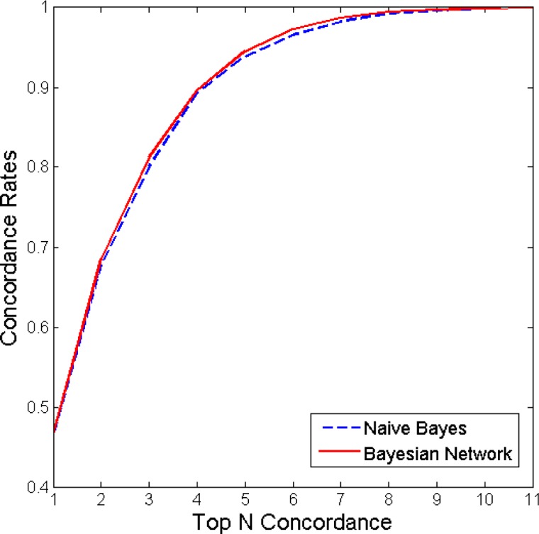
Concordance results of the NB algorithm and the BN learned with MC³. As can be seen from the figure, the BN learned with MC³ only marginally outperformed the NB algorithm.

The graph in Figure 3 can be interpreted in a way that is similar to a ROC curve, in that the closer the curve is to the upper left corner, the more successful the classifier is in matching the treatment decisions recorded in the dataset. Based on these results, we see that the MC³ BN and NB algorithms perform similarly at ‘Top 1 concordance’, with a concordance rate of approximately 0.46. We can observe that at Top 3 concordance, the MC³ BN achieves a concordance rate of 0.81, while the NB algorithm falls slightly behind with a concordance rate of 0.80. In this definition, concordance should not be confused with accuracy. The recorded treatments, with which we are comparing the outcomes of the classifiers, do not necessarily represent the gold standard results.

In Figure 4, we compare the 1-year-survival percentages of the discordant and concordant cases for the MC³ BN results. We can see that at Top 1 concordance, the cases which have been flagged up by the classifier as discordant have an approximately 15% (45% - 30%) less 1-year-survival chance compared to the concordant ones, where the classifier was in agreement with the clinicians’ choice.

Figure 4.

1-year survival percentages of the concordant and discordant cases plotted with respect to the number of top classifier recommendations being taken into account.

If we relax our search boundaries for concordance to include the top N recommendations, we see that while the 1-year-survival-rates increase for the discordant cases, they decrease for the concordant ones and that they intersect at around the Top 6 concordance level. The value at which this intersection occurs is, unsurprisingly, near the prior probability of 1-year-survival for the dataset, i.e. 37/100 = 0.37. Starting from the Top 6 concordance level, the survival percentages for concordant cases stabilise around the population prior. However, the survival percentages for the discordant cases begin to fluctuate heavily. This can be due to the fact that as the size of the discordant set decreases with N, it becomes statistically insignificant at around Top 7 concordance level.

We have also investigated the concordance rates per treatment type in order to highlight any treatment types that the BN is bad at predicting. Figure 5.a and 5.b project these concordance rates on treatment distributions at Top 1 concordance and Top 3 concordance levels. The height of the bars represent the frequency of the treatment type appearing in the dataset and the dark blue portions of each bar indicate the concordant cases for that specific treatment type.

Figure 5.

Distribution of the concordant and discordant cases with respect to treatment type at (a) Top 1 concordance level and (b) Top 3 concordance level

As seen in Figure 5.a, the BN is successful at predicting Treatment 1 (Surgery) and Treatment 3 (Chemotherapy) with high rates of concordance for both treatment types. This is not surprising since Treatment 1 (Surgery) and Treatment 3 (Chemotherapy) are among the 3 most frequent treatments given to patients, as indicated by their bar heights, and so we can expect the BN to be well-trained to pick up these treatment types. The unexpected finding here is that the Top 1 concordance for Treatment 2 (Radiotherapy) is surprisingly low although we would expect the same high concordance for this treatment type as well. This may be due to some missing variable(s) that we have not included in our 9-variable set that the experiments in this paper focus on. It is also interesting to see that despite its low performance at Top 1 concordance, Treatment 2 (Radiotherapy) catches up with Treatments 1 and 3 with a concordance rate of approximately 95% when the top 3 treatments are taken into account, as shown in Figure 5.b.

Both Figure 5.a and Figure 5.b reveal that despite being respectively the 4^th and the 5^th most common treatment decisions in the database, Treatment 5 (Palliative Care) and Treatment 6 (Active Monitoring) have low rates of concordance. It can be interpreted that the Bayesian classifier does not regard active monitoring as a treatment option that maximises the probability of 1-year-survival and therefore flags the recorded ‘Active Monitoring’ treatment decisions more often than others. This can partially be explained by the fact that Active Monitoring is not a curative treatment option and therefore may not have a very strong statistical influence on 1-year-survival. A similar remark can be made for treatment type 5, i.e. Palliative Care. Similar to Active Monitoring, Palliative Care is not a curative treatment and therefore may need to be excluded from a Bayesian query which is run to determine the treatment type that maximises 1-year-survival.

For the less commonly encountered treatment types, such as Treatment 4 (Brachytherapy), Treatment 9 (Induction chemotherapy before surgery) and Treatment 10 (Neo-adjuvant chemotherapy and surgery), we observed that concordance rates were quite low. This may be due to the rarity of these treatment decisions in the database, which results in low prior probabilities for these Treatment node states in the BN. An alternative explanation, which is not mutually exclusive with the first one, would be that there are other variables outside our 9-variable set, which inform the decisions for these treatment types.

Conclusions and Future Work

In this paper, we reported our preliminary results on the performance of different Bayesian techniques in prognosis prediction and treatment recommendation for lung cancer. We have carried out these experiments to inform our decision regarding the choice of the Bayesian techniques to integrate into our online clinical decision support application, Lung Cancer Assistant, which is under development. We based our experiments on a 9-variable and fully observed subset of the English national lung cancer dataset (LUCADA), which included 36480 patients.

Our first set of experiments focused on 1-year-survival prediction. The results indicate that NB marginally outperformed the BNs, structured using the MC³ and K2 algorithms. This may be due to the fact that the subset we have taken in this paper was fully-observed, making handling missing data – which BNs are suitable for - inessential. In our second set of experiments, we defined treatment as our outcome variable and focused on recommending the treatment that maximises the probability of survival for the patient. We observed that the BN marginally outperformed the NB in terms of concordance with the recorded treatments. The classifier’s top recommendation matched the actual recorded treatment in LUCADA only 46% of the time. The 1-year-survival rate of these concordant cases was approximately 15% higher than the discordant ones, which outlines that the cases flagged up as ‘discordant’ had significantly poorer survival outcomes. When we relaxed the matching-constraint to include the top 3 recommendations, the classifier achieved 81% concordance with the recorded treatments.

We observed that the classifier tended to selectively disagree with two major types of recorded treatment decisions in the dataset: 1) Active Monitoring and 2) Palliative Care. For these non-curative treatments, we can argue that 1-year-survival is not a relevant outcome metric and therefore such cases should be evaluated or classified based on a different outcome metric. We also observed that the concordance levels for the less common treatment types in the database were in general lower than the more common ones, such as Surgery and Chemotherapy. The only exception to this was Radiotherapy, which had a low concordance rate of 0.3 at Top 1 concordance level, despite being the second most frequent treatment decision in the dataset. For such cases, which the BN classifier performs relatively poorly, the guideline-based decision support mode of Lung Cancer Assistant may complement the classifier approach and provide a more complete picture, enabling multi-criteria decision support.

The primary limitation to our study was our selection of a fully-observed subset that included only 9 variables from the entire LUCADA dataset. Despite the fact that these 9 variables were picked based on their frequent appearance in the clinical guideline documents, the treatment selection results hint that they probably do not constitute a comprehensive variable set for the task at hand and that a more formal, statistical feature selection step, which takes into account all data items in the database, is necessary. Furthermore, in the structure learning step, while the DAG’s returned with the MC³ algorithm (Figure 1.a and Figure 1.b) were similar, they were different than the DAG returned by the K2 algorithm. In our current study, we are adopting a structure learning approach that makes use of both the MC³ and K2 algorithms sequentially, similar to what Oh et al. suggest in [22]. Also, we plan to investigate the options of active structure learning [25] through which we can incorporate expert knowledge and different variable orders to aid the process. Finally, we plan to investigate classifier performances based on not only 1-year, but also 2-year and 3-year survival cut-offs which may produce different results.

In conclusion, we believe the preliminary results in this paper are valuable not only in determining the direction of our research in identifying the Bayesian technique that represents the LUCADA dataset most accurately but also in better identifying the shortcomings of a decision support approach that is strictly machine-learning-based.

References

- [1].National Collaborating Centre for Cancer The diagnosis and treatment of lung cancer (update) 2011. [PubMed]
- [2].Lim E, et al. Guidelines on the radical management of patients with lung cancer. Oct, 2010. [DOI] [PubMed]
- [3].a Cruz J, Wishart DS. Applications of machine learning in cancer prediction and prognosis. Cancer informatics. 2006 Jan;2:59–77. [PMC free article] [PubMed] [Google Scholar]
- [4].Heckerman D. A Tutorial on Learning with Bayesian Networks. 1996.
- [5].Daly R, Shen Q, Aitken S. Learning Bayesian networks: approaches and issues. The Knowledge Engineering Review. 2011 May;26(2):99–157. [Google Scholar]
- [6].Lucas PJF, van der Gaag LC, Abu-Hanna A. Bayesian networks in biomedicine and health-care. Artificial intelligence in medicine. 2004 Mar;30(3):201–14. doi: 10.1016/j.artmed.2003.11.001. [DOI] [PubMed] [Google Scholar]
- [7].Rish I. An empirical study of the naive Bayes classifier. IJCAI 2001. 2001.
- [8].Dekker A, et al. Survival Prediction in Lung Cancer Treated with Radiotherapy: Bayesian Networks vs. Support Vector Machines in Handling Missing Data. 2009 International Conference on Machine Learning and Applications; Dec. 2009.pp. 494–497. [Google Scholar]
- [9].The National Lung Cancer Audit The National Clinical Lung Cancer Audit (LUCADA) Data Manual. 2010.
- [10].International Classification of Diseases for Oncology: Morphology of Neoplasms, Edition 3. 2000. [Online]. Available: http://www.wolfbane.com/icd/icdo3.htm.
- [11].WHO International Statistical Classification of Diseases and Related Health Problems 10th Revision. 2010. [Online]. Available: http://apps.who.int/classifications/apps/icd/icd10online/
- [12].Mitchell TM. Generative and Discriminative Classifiers: Naive Bayes and Logistic Regression. Machine Learning. 2010:1–17. [Google Scholar]
- [13].Cooper GF, Hennings-Yeomans P, Visweswaran S, Barmada M. An efficient Bayesian Method for predicting clinical outcomes from genome-wide data. AMIA Annual Symposium proceedings; Jan. 2010; 2010. pp. 127–31. [PMC free article] [PubMed] [Google Scholar]
- [14].Korb K, Nicholson A. Bayesian Artificial Intelligence. 2004;52(2) [Google Scholar]
- [15].Pearl J, Russell S. Bayesian Networks. 2000.
- [16].Murphy K. The Bayes Net Toolbox for MatLab. 2001.
- [17].Madigan D, York J. Bayesian Graphical Models for Discrete Data. International Statistical Review. 1995;63(2):215–232. [Google Scholar]
- [18].Murphy K. Learning Bayes net Structure from sparse data sets. 2001.
- [19].Cooper GF, Herskovits E. A Bayesian Method for the Induction of Probabilistic Networks from Data. 1992;347:309–347. [Google Scholar]
- [20].Huang C. Inference in belief networks: A procedural guide. International Journal of Approximate Reasoning. 1996 Oct;15(3):225–263. [Google Scholar]
- [21].Lauritzen S, Spiegelhalter D. Local Computations with Probabilities on Graphical Structures and their Application to Expert Systems. Journal of the Royal Statistical Society. 1988;50(2):157–224. [Google Scholar]
- [22].Murphy K. Active Learning of Causal Bayes net Structure. 2001.
- [23].Larjo A, et al. Active Learning of Bayesian Networks in a Realistic Setting. 2011. North.
- [24].Sikonja MR. Theoretical and Empirical Analysis of ReliefF and RReliefF. Machine Learning. 2003:23–69. [Google Scholar]
- [25].Oh J, et al. A Bayesian network approach for modelling local failure in lung cancer. Physics in Medicine and Biology. 2011;56:1635–1651. doi: 10.1088/0031-9155/56/6/008. [DOI] [PMC free article] [PubMed] [Google Scholar]