A Semi-Automated Quantification of Pulmonary Artery Dimensions in Computed Tomography Angiography Images

Abstract

Quantifying vascular dimensions may provide a non-invasive means of diagnosing a variety of vascular diseases, including pulmonary hypertension, a progressive, potentially fatal disease that results in the remodeling of the pulmonary vasculature. Currently the gold standard for diagnosis of pulmonary hypertension is through right heart catheterization, an invasive and costly procedure. Since pulmonary hypertension is associated with the remodeling of the pulmonary arteries, quantifying vascular geometry as depicted in tomographic imaging may provide a non-invasive diagnostic technique. In this work we explore a semi-automated method for quantifying pulmonary vascular geometry with the intention of using such measurements in the future for diagnosing pulmonary hypertension.

Introduction

For years researchers have been trying to find an alternative, noninvasive method for diagnosing the presence of pulmonary hypertension (PH) [1–4]. The current “gold standard” diagnosis is right heart catheterization (RHC), which is an invasive and costly procedure that carries a risk for the patient. A promising alternative approach to this problem is to find a way of using the information in computed tomography (CT) images that is as reliable as the results obtained through RHC.

PH occurs when there is an abnormal elevation in the pressure of the pulmonary artery. The pressure is indicative of PH when it is either greater than 25 mmHg when at rest or greater than 30 mmHg when exercising [5]. This increase in pressure is usually caused by vascular remodeling, thrombosis, and vasoconstriction. This is often a lethal combination because the progressive nature of the disease leads to right ventricular dilatation and hypertrophy, resulting in heart failure [1].

The vascular remodeling associated with PH results in a marked change in the relative diameters of the pulmonary arteries. In a healthy person, the total cross-sectional area of the pulmonary arterial vasculature increases with branching depth. In a patient with PH, however, the total cross-sectional area decreases with branching depth. Thus a potential means of diagnosing PH is to compare the relative diameters of the pulmonary arterial trunk to the diameters of the left and right pulmonary arteries. In this paper we present our preliminary results for automated vascular geometry quantification from CT images that will ultimately form the basis for diagnosing pulmonary hypertension. Using CT images obtained on subjects negative for PH, we validated our automated measurements by comparing them to manually obtained diameter measurements.

Methods

We randomly selected 10 normal CT pulmonary angiography (CTPA) exams from our data bank. The exams were determined to be negative with respect to both pulmonary embolism (the indication for the exams) and to PH by examining the accompanying dictated radiology reports.

For each case, human observers manually quantified the vascular geometry. Independent of these measurements, models of the pulmonary arterial vasculature were generated and used to quantify vascular geometry in the same cases. These steps are described below.

Make manual measurements of the pulmonary vasculature

In order to determine how well the automated measurements were performing, we first needed to generate a reference standard for comparison. We did this by first going though each of the exams and identifying the slices by selecting those at the mid-most section of the vessel. These slices were then used to measure the diameters of the pulmonary trunk and the right and left main pulmonary arteries (reviewer 0). We wrote a Python (www.python.org) script to isolate these slices for manual quantification. Manual quantification was performed by four independent observers using OsiriX (http://www.osirix-viewer.com/). For the identified slice, each observer used a linear ROI (region of interest) tool to measure the diameter of the appropriate vessel at the estimated midpoint. Each observer was blind to both the other reviewers’ results and to the quantification from the vascular models. Figures 1a–b show one of the normal cases on which the measurements were made using OsiriX.

Figures 1a–b).

Example of manual the measurements made in OsiriX. Left) right main pulmonary artery and right) left main pulmonary artery.

Model the pulmonary vasculature

The first step in the vascular model generation process is to segment the pulmonary arteries within the CT images. Automated segmentation of medical images remains a challenging problem, and most current applications rely on semi-automated methods. For example, the Vascular Modeling Toolkit (VMTK) has the user specify beginning and ending points for each vascular path to be segmented (http://www.vmtk.org/). We used the ITK-Snap tool [6] to perform an intensity-based level set segmentation. The user specified a seed point and intensity mapping parameters. The parameters were manually adjusted to minimize bleeding of the segmentation into the surrounding anatomy, although some manual editing was still required to eliminate bleeding into other vascular structures (e.g., “bleeding” from the right pulmonary artery into the vena cava). Finally, median filtering and mathematical morphology were used to clean the segmentations prior to model formation.

The second step is to generate the skeletons for each of the segmentations. The skeleton is composed of lines, one voxel thick, that are at the center of the vessels. We used an existing ITK-based parallel thinning algorithm (itkBinaryThinningImageFilter3D) [7] for extracting the skeleton from the discrete space. The goal is to iteratively remove the object’s surface until only the centerlines remain. An example segmentation and the resulting skeleton is shown in Figure 2.

Figure 2.

(Left) Surface rendering of the segmentation obtained with ITK-Snap. (Right) Illustration of the skeleton achieved from the segmentation using parallel thinning.

The skeleton is simply an image of unordered voxels. In order to make our measurements, we must first transform these unordered voxels into a structure that represents the underlying anatomy. We did this by creating vascular graphs in which nodes of the graphs are vascular bifurcations and terminations (endpoints) and edges of the graphs are the vessel centerlines. This is a multi-step process that we now describe.

First, we created an undirected graph with every voxel in the skeleton being a node in the graph. Edges were added between any nodes coexisting within a 3×3×3 neighborhood. From this, undirected graph bifurcations and endpoints were recognized by the node degree: degree-three nodes are bifurcations, degree-two nodes are centerlines, and, degree-one nodes are endpoints. This is illustrated in Figure 3.

Figure 3.

Example of an undirected graph generated from a skeleton image. Here blue nodes are bifurcations, green nodes are centerlines, and red nodes are endpoints.

Second, a directed graph was generated from the undirected graph. A root node was required for the directed graph and we selected the undirected graph node with the highest distance from edge (DFE) value as the root. The DFE was calculated using the city distance transform. Expanding out from the root, all bifurcation and endpoint nodes in the undirected graph were added as nodes in the directed graph with the collection of degree-two nodes (centerlines) forming the directed edge between the nodes. Each node is labeled with the (i,j,k) coordinate of the skeletal image voxel from which the node was obtained.

Third, because of imperfections in the segmentation, the resulting directed graph may have a number of edges leading to false endpoint nodes. To clean the graph we deleted any edge that was shorter than five voxels. This naïve rule was often not adequate, so we manually deleted extraneous edges. We are experimenting with machine learning techniques to create more comprehensive pruning rules.

Finally, the edges of the pruned graph were fit with a least-squares cubic spline. The spline fit provides a smooth function that will later be used to capture vascular features from the segmented image. An example of a fitted graph is shown in Figure 4.

Figure 4.

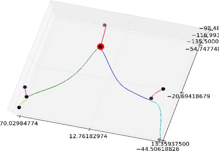
An example of a directed graph that has had the centerlines fit with a least-squared cubic spline. The root of the graph is highlighted in red. Note that in this case the selected root corresponds to the bifurcation of the pulmonary trunk into the left and right pulmonary arteries.

Making automated measurements for comparison

In order to make automated measurements from an ordered graph, we must first match the graph to the anatomy of interest. Although originally motivated by the need to recognize the pulmonary trunk, our heuristic of setting the root node to be the node with the maximum distance from edge was not sufficiently accurate, since, as illustrated with Figure 5, the root node was placed at the bifurcation rather than in the trunk (other incorrect locations were also observed). For identification of the pulmonary trunk, we used the approximate symmetry of the pulmonary arterial tree to identify the directed graph node best matching the pulmonary trunk. Since the pulmonary trunk lies near the center of the left-right (x) direction of the tree, the root node should lie close to the median (or mean) x coordinate for the nodes. Selecting the node closest to the mean x value correctly identified the pulmonary trunk node in all ten of our test cases. The graph was then “re-rooted” with the new root value. The re-rooted graph from Figure 5 is shown in Figure 6. The pulmonary trunk was then defined as the edge between the root node and its child bifurcation. The left and right pulmonary arteries were then the edges exiting this child bifurcation.

Figure 6.

(Left) Graph from Figure 5 with surface points matched to each edge. (Right) Surface points mapped to the plane orthogonal to the midpoint of the centerline. These mapped points form the basis for our diameter measurements.

With the graph matched to anatomy, we went back to the original segmentation and matched each surface voxel to the nearest edge. Finally, the spline-fit to each edge was used to define a plane at each point along the centerline that was orthogonal to the local direction of the centerline. The mapped surface points for each edge were then mapped to one of these orthogonal planes. These steps are illustrated in Figure 6. The average distance between centerline and surface points in the orthogonal plane then define a local radius measure.

Statistical Comparisons

We wanted to determine if there was a statistically significant difference between the manual and the automated measurements. We calculated the mean (X̄), variance (S²) and standard deviation (S) for each group for each vessel. We then calculated the experimental t value for comparison to the t-critical [8]. The actual calculations of these values were verified using an applet generated at the National and Kapodistrian University of Athens in Greece and maintained by Professor Efstathiou [9]. These values can be found in table 1 in the results section..

When determining statistical significance, if the calculated t value was less than the critical t value, then there was no difference in the means of the automated and manual measurements. If the calculated t value was greater than the critical value, then the two means were significantly different, and the null was rejected [8].

Results

In the following table, each vessel has three columns. First are the manual measurements, which are the average measurement value across four reviewers for each case. Second, are the automated measurements and third, is the difference between the two measurements (the automated subtracted from the manual measurement value). These values are followed by the summary statistics, mean (X̄), variance (S²), standard deviation (S) and calculated t-values.

Table 1.

Summary of the measurement values by case.

	Manual PT	Auto PT	PT DIFF	Manual RMPA	Auto RMPA	RMPA DIFF	Manual LMPA	Auto LMPA	LMPA DIFF
3	3.01	3.25	−0.24	2.34	2.67	−0.33	2.47	2.44	0.02
9	2.79	2.84	−0.04	2.02	2.08	−0.06	1.92	2.01	−0.09
57	2.39	2.74	−0.35	1.99	2.59	−0.60	2.01	2.59	−0.58
105	2.67	2.56	−0.11	1.80	1.65	−0.15	1.65	1.77	−0.12
119	3.09	3.05	0.04	2.16	2.18	−0.02	1.88	1.81	0.06
148	3.13	3.04	0.08	2.16	2.36	−0.20	2.61	2.38	0.23
156	1.78	2.06	−0.28	1.53	1.22	0.30	1.32	1.41	−0.08
201	3.45	3.62	−0.17	2.35	2.41	−0.06	2.01	2.19	−0.18
202	2.24	2.59	−0.34	1.70	1.58	0.12	1.77	1.89	−0.12
207	2.67	3.68	−1.01	2.25	2.63	−0.39	2.31	2.72	−0.41
X̄	2.72	2.94	−0.22	2.03	2.14	−0.11	1.99	2.12	−0.13
S2	0.14			0.08			0.06
S	0.46	0.47		0.28	0.5		0.37	0.41
texp	1.053			0.647			0.7784

Discussion

When reviewing our statistical data in reference to tables 1–3, we found that for all three vessels (the pulmonary trunk, the RMPA and the LMPA) there was no significant difference between the manual measurement means and the automated measurement means. We compared the calculated t values with the t critical value at 95% = 1.734 [8], and each of the t-values was less than 1.734; for that reason, the null of no difference between the means cannot be rejected. This is encouraging, because our primary goal is to identify a method for obtaining these values in an automatic method that is as accurate as manual methods.

In 22 out of 30 measurements (73%) the automated measurement was greater than the manual measurement. There are several factors that can contribute to differences in the measurements. First, there can be differences in the visual threshold used by the observers and the threshold used in the segmentation. Second, the manual measurements were made in 2D, whereas the automated measurements were made in 3D. Third, since the manual and automated measurements were made completely independently, the measurements were not necessarily taken at the same location of each vessel. There is one case in particular that seems to be an outlier: the pulmonary trunk measurement for case 207, where there is a little over 1 cm difference in size, shows the greatest difference across all the measurements. The cause for this difference is unclear and will need to be addressed in future work.

There are several limitations to this current study. First, although we are trying to develop an automated method, we relied on a semi-automatic segmentation technique. Automatic segmentation is recognized as being a very challenging problem. However, we hope that in the future our manual segmentation can form the basis for automated template-driven segmentations. Second, we present only a small number of cases; using such a small dataset could result in the presence of false negatives resulting in the incorrect rejection of the null hypothesis. This is a proof of concept, and we are currently compiling results on a larger data set to eliminate this potential limitation. Finally, these results are only from negative cases. Because our collection of PH cases is small, we have limited our preliminary algorithm development to negative cases.

Conclusion

We have developed a semi-automated method for the measurement of the main vessel diameters in the pulmonary vasculature that showed no significant difference when compared to manual measurements. Additional work remains in using these measurements to diagnosis pulmonary hypertension. However, we believe this work represents an important foundational first step in achieving this goal.

References

- 1.Chan AL, et al. Novel computed tomographic chest metrics to detect pulmonary hypertension. BMC Medical Imaging. 2011;11:7. doi: 10.1186/1471-2342-11-7. [DOI] [PMC free article] [PubMed] [Google Scholar]
- 2.Haimovici JBA, et al. Relationship between pulmonary artery diameter at computed tomography and pulmonary artery pressures at right-sided heart catheterization. Academic Radiology. 1997;4(5):327–334. doi: 10.1016/s1076-6332(97)80111-0. [DOI] [PubMed] [Google Scholar]
- 3.Grubstein A, et al. Computed tomography angiography in pulmonary hypertension. Isr Med Assoc J. 2008;10(2):117–20. [PubMed] [Google Scholar]
- 4.Edwards PD, Bull RK, Coulden R. CT measurement of main pulmonary artery diameter. Br J Radiol. 1998;71(850):1018–20. doi: 10.1259/bjr.71.850.10211060. [DOI] [PubMed] [Google Scholar]
- 5.Hegewald MJ, Markewitz B, Elliott CG. Pulmonary hypertension: clinical manifestations, classification and diagnosis. International journal of clinical practice. Supplement. 2007;(156):5–14. doi: 10.1111/j.1742-1241.2007.01479.x. [DOI] [PubMed] [Google Scholar]
- 6.Ibanez Luis, et al. Insight Tool Kit. Kitware Inc; 2005. [Google Scholar]
- 7.Homann H. Implementaion of a 3D thinning algorithm. The Insight Journal. 2007 [Google Scholar]
- 8.Rosner B. Fundamentals of Bostatistics. 6th ed. United States of America: Thompson Brooks/Cole; 2006. [Google Scholar]
- 9.Efstathiou CE. Student’s t-test comparison of two means. 2012. [cited 2012 March 14, 2012. Available from: http://www.chem.uoa.gr/applets/AppletTtest/Appl_Ttest2.html.s.