Abstract
We present a novel cosine series representation for encoding fiber bundles consisting of multiple 3D curves. The coordinates of curves are parameterized as coefficients of cosine series expansion. We address the issue of registration, averaging and statistical inference on curves in a unified Hilbert space framework. Unlike traditional splines, the proposed method does not have internal knots and explicitly represents curves as a linear combination of cosine basis. This simplicity in the representation enables us to design statistical models, register curves and perform subsequent analysis in a more unified statistical framework than splines.
The proposed representation is applied in characterizing abnormal shape of white matter fiber tracts passing through the splenium of the corpus callosum in autistic subjects. For an arbitrary tract, a 19 degree expansion is usually found to be sufficient to reconstruct the tract with 60 parameters.
Keywords and phrases: Cosine series representation, Curve registration, Curve modeling, Fourier descriptor, Diffusion tensor imaging, White matter tracts
1. INTRODUCTION
Diffusion tensor imaging (DTI) has been used to characterize the microstructure of biological tissues using magnitude, anisotropy and aniotropic orientation associated with diffusion [2]. It is assumed that the direction of greatest diffusivity is most likely aligned to the local orientation of the white matter fibers. White matter tractography offers the unique opportunity to characterize the trajectories of white matter fiber bundles noninvasively in the brain. Whole brain tractography studies routinely generate up to half million tracts per brain. Various deterministic tractography have been used to visualize and map out major white matter pathways in individuals and brain atlases [3, 8, 14, 31, 34, 35, 43, 47]; however, tractography data can be challenging to interpret and quantify. Recent efforts have attempted to cluster [36] and automatically segment white matter tracts [37] as well as characterize tract shape parameters [4]. Many of these techniques can be quite computationally demanding. Clearly efficient methods for representing tract shape, regional tract segmentation and clustering, tract registration and quantification would be of tremendous value to researchers.
In this paper, we present a novel approach for parameterizing white matter fiber tract shapes using a new Fourier descriptor. Fourier descriptors have been around for many decades for modeling mainly planar curves [38, 42]. They have been previously used to classify tracts [4]. The Fourier coefficients are computed by the Fourier transform that involves the both sine and cosine series expansion. Then the sum of the squared coefficients are obtained up to degree 30 for each tract and the k-means clustering is used to classify the fibers globally. Our approach differs from [4] in that we obtain local shape information employing cosine series only, without using both the cosine and sine series making our representation more compact. Using our new compact representation, we demonstrate how to quantify abnormal pattern of white matter fibers passing through the splenium of the corpus callosum for autistic subjects.
Splines have also been widely used for modeling and matching 3D curves [13, 23, 29]. Unfortunately, splines are not easy to model and to manipulate explicitly compared to Fourier descriptors, due to the introduction of internal knots. In Clayden et al. [13], the cubic-B spline is used to parameterize the median of a set of tracts for tract dispersion modeling. Matching two splines with different numbers of knots is not computationally trivial and has been solved using a sequence of ad-hoc approaches. In Gruen et al. [23], the optimal displacement of two cubic spline curves are obtained by minimizing the sum of squared Euclidean distances. The minimization is nonlinear so an iterative updating scheme is used. On the other hand, there is no need for any numerical optimization in obtaining the matching in our method due to the very nature of the Hilbert space framework. We will show that the optimal matching is embedded in the representation itself. Instead of using the squared distance of coordinates, others have used the curvature and torsion as features to minimized to match curves [25, 29, 33]. In particular, Corouge et al. used cubic B-splines for representation fiber tracts and then curvature and torsion were used as [15].
In summary, this paper makes the following contibutions: (i) Introduce a more compact Fourier descriptor that uses only the half the number of basis; (ii) Show that curve matching can be done without any numerical optimization; (iii) Show how to perform a statistical inference on fiber bundles consisting of multiple 3D curves. The MATLAB implementation for the cosine series representation can be found in brainimaging.waisman.wisc.edu/~chung/tracts.
2. 3D CURVE MODELING
We are interested in encoding a smooth curve
 consisting of n noisy ordered control points p1, …, pn. Consider a mapping ζ−1 that maps the control point pj onto the unit interval [0, 1] as
| (1) |
This is the ratio of the arc-length from the point p1 to pj, to p1 to pn. We let this ratio to be tj. We assume ζ−1(p1) = 0. The ordering of the control points is also required in obtaining smooth one-to-one mapping. Then we parameterize the smooth inverse map
as a linear combination of smooth basis functions.
2.1 Eigenfunctions of Laplacian
Consider the space of square integrable functions in [0, 1] denoted by
 [0, 1]. Let us solve the eigenequation
| (2) |
in
 [0, 1] with 1D Laplacian
. The eigenfunctions ψ0, ψ1, … form an orthonormal basis in
 [0, 1]. Instead of solving (2) in the domain [0, 1], we solve it in the larger domain ℝ with the periodic constraint
| (3) |
The eigenfunctions are then Fourier sine and cosine basis
with the corresponding eigenvalues λl = l2π2. The period 2 constraint forces the basis function expansion to be only valid in the intervals …, [−2, −1], [0, 1], [2, 3], … while there are gaps in …, (−1, 0), (1, 2), (3, 4), …. We can fill the gap by padding with zeros but this will result in the Gibbs phenomenon (ringing artifacts) [10] at the points of jump discontinuities.
One way of filling the gap automatically while making the function continuous across the whole intervals is by putting the constraint of evenness, i.e.
| (4) |
Then the only eigenfunctions satisfying two constraints (3) and (4) are the cosine basis of the form
| (5) |
with the corresponding eigenvalues λl = l2π2 for integers l > 0. The constant is introduced to make the eigenfunctions orthonormal in [0, 1] with respect to the inner product
| (6) |
where δlm is the Dirac-delta function. With respect to the inner product, the norm ||·|| is then defined as
2.2 Cosine representation
Model
Denote the coordinates of ζ as (ζ1, ζ2, ζ3). Then each coordinate is modeled as
| (7) |
where μi is an unknown smooth function to be estimated and εi is a zero mean random field, possibly Gaussian. Instead of estimating μi in
 [0, 1], we estimate in a smaller subspace
 , which is spanned by up to the k-th degree eigenfunctions:
Then the least squares estimation of μi in
 is given by
Obviously, the minimization is simply given as the k-th degree expansion:
| (8) |
With this motivation in mind, we have the following k-th degree cosine series representation for a 3D curve:
| (9) |
where εi is a zero mean random field. It is also possible to have slightly different but equivalent model that will be used for statistical inference. Assuming Gaussian random field, εi can be expanded using the given basis ψl as follows.
where are possibly correlated Gaussian and ei is the residual error field that cab be neglected in practice. This is the direct consequence of the Karhunen-Loeve expansion [1, 16, 30, 46]. Therefore we can equivalently model (9) as
| (10) |
where .
Estimation
We only observe the curve
 in finite number of control points ζj (t1), …, ζj (tn) so we further need to estimate the Fourier coefficient cli = 〈ζi, ψl〉 as follows. At control points we have normal equations
where
The coefficients are simultaneously estimated in the least squares fashion as
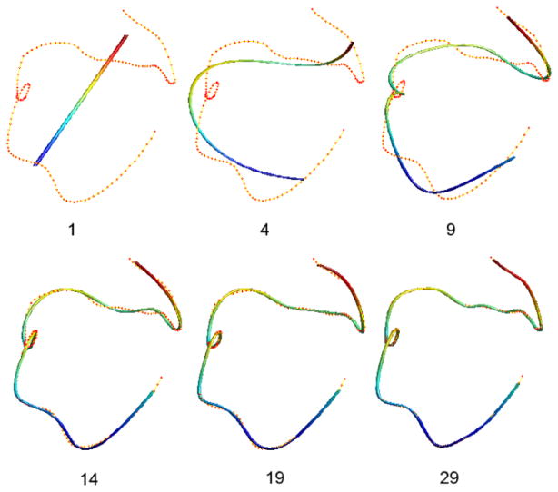
The proposed least squares estimation technique avoids using the Fourier transform (FT) [4, 7, 24]. The drawback of the FT is the need for a predefined regular grid system so some sort of interpolation is needed. The advantage of the cosine representation is that, instead of recording the coordinates of all control points, we only need to record 3 · (k + 1) number of parameters for all possible tract shape. This is a substantial data reduction considering that the average number of control points is 105 (315 parameters). We recommend readers to use 10 ≤ k ≤ 30 degrees for most applications. In our application, we have used degree k = 19 through out the paper (Figure 2). This gives the average absolute error of 0.26mm along the tract. The MATLAB code for performing the least squares estimation can be obtained from brainimaging.waisman.wisc.edu/~chung/tracts.
Figure 2.
Cosine representation of a tract at various degrees. Red dots are control points obtained from a streamline based tractography. The degree 1 representation is a straight line that fits all the control points in a least squares fashion. The degree 19 representation is used through the paper.
2.3 Optimal representation
We have explored the possibly of choosing the optimal number of basis using a stepwise model selection framework. This model selection framework for Fourier descriptors was first presented in [10, 11]. Although increasing the degree of the representation increases the goodness-of-fit, it also increases the number of estimated coefficients linearly. So it is necessary to stop the series expansion at the degree where the goodness-of-fit and the number of coefficients balance out.
Assuming up to the (k−1)-degree representation is proper in (9), we determine if adding the k-degree term is statistically significant by testing
Let the k-th degree sum of squared errors (SSE) for the i-th coordinate be
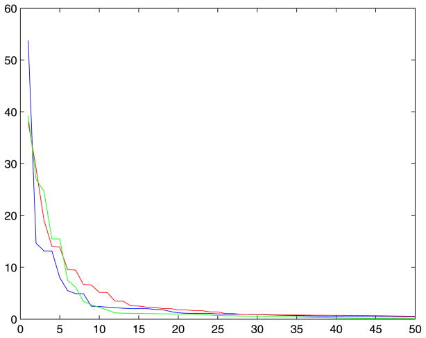
where are the least squares estimation. The plot of SSE for varying degree 1 ≤ k ≤ 50 a particular tract is shown in Figure 3. As the degree k increases, SSE decreases until it flattens out. So it is reasonable to stop the series expansion when the decrease in SSE is no longer significant. Under H0, the test statistic F follows
Figure 3.
The plot of the sum of squired errors (SSE) for degree between 1 and 50. SSE rapidly flattens out around degree 15–20. The blue, red and green lines are the SSE plot of x, y and z coordinates respectively.
the F -distribution with 1 and n − k − 2 degrees of freedom. We compute the F statistic at each degree and stop increasing the degree of expansion if the corresponding p-value first becomes bigger than the pre-specified significance α = 0.01. The forward model selection framework hierarchically builds the cosine series representation from lower to higher degree.
In many Fourier descriptor and spherical harmonic representation literature, the issue of the optimal degree has not been addressed properly and the degree is simply selected based on a pre-specified error bound [7, 19, 24, 40, 41]. Since the stepwise model selection framework chooses the optimal degree for each coordinate separately, we have chosen the maximum of optimal degrees for all coordinates. The optimal degree changes if a different tract is chosen. For instance, the optimal degrees for 4,987 randomly chosen whole brain white matter tracts longer than 30mm are 13.94±7.02 and the upper 80 percentile is approximately 19. For simplicity in numerical implementation and inference, it is crucial to choose the same fixed degree for all tracts. We do not want to choose the degree 14 as optimal since then about 50% of tracts will not be represented optimally. Therefore, we have chosen the degree corresponding to the upper 80 percentile to be used through the paper.
We have also checked if the optimal degree is related to the length but found no relation. The correlation between the length of tracts and the optimal degree is 0.06, which is statistically insignificant. The increased degree should correspond to the increased curvature and bending rather than the the length of tracts. This issue is left as a future research and we did not pursue it any further.
3. 3D FIBER BUNDLE MODELING
Using the cosine series representation, we show how to analyze a collection of fiber bundles consisting of similarly shaped curves. The ability to register one tract to another tract is necessary to establish anatomical correspondence for a subsequent population study. Since curves are represented as combinations of cosine functions, the registration will be formulated as a minimization problem in the subspace
 which avoids brute-force style numerical optimization schemes given in [23, 25, 29, 33, 39]. This simplicity makes the cosine series representation more well suited than the usual spline representation of curves [23] in subsequent statistical analysis.
3.1 Registering 3D curves
With the abuse of notations, we will interchangeably use curves to be estimated and their estimation with the same notations when the meaning is clear. Let the cosine series representation of two curves η and ζ be
| (11) |
| (12) |
where ηl and ζ are the Fourier coefficient vectors.
Consider the displacement vector field u = (u1, u2, u3) that is required to register ζ to η. We will determine an optimal displacement u such that the discrepancy between the deformed curve ζ+u and η is minimized with respect to a certain discrepancy measure ρ. The discrepancy measure ρ between η and ζ are defined as the integral of the sum of squared distance:
| (13) |
The discrepancy ρ can be further simplified as
We have used the orthogonality condition (6) to simplify the expression. The algebraic manipulation will show that the optimal displacement u*, which minimizes the discrepancy between ζ + u and η, is given by
| (14) |
| (15) |
The proof requires substituting
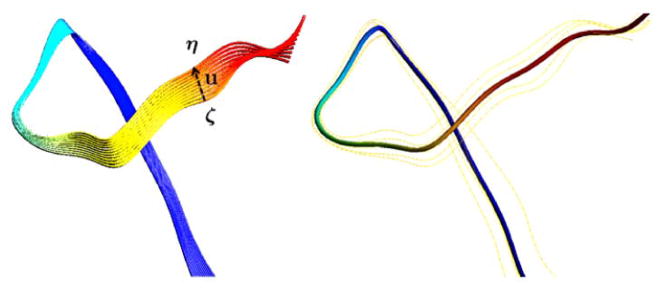
in the expression (14), which becomes the unconstrained positive definite quadratic program with respect to variables ul = (ul1, ul2, ul3). So the global minimum always exists and obtained when ρ(ζ+ u*, η) = 0. Figure 4 shows the schematic view of registration.
Figure 4.
Left: the curve ζ is registered to η by the displacement vector field u. The other intermediate curves are generated by plotting ζ + αu* with α ∈ [0, 1] to show how the different amount of displacement deforms the curve ζ. Right: the average of a fiber bundle consisting of 5 tracts.
The simplicity of our approach is that curve registration is done by simply matching the corresponding Fourier coefficients without any sort of numerical optimization as in spline curve matching.
3.2 Inference on fiber bundles
Based on the idea of registering tracts by matching coefficients, we construct the average of a white fiber bundle consisting of m curves ζ1, …, ζm by finding the optimal curve that minimizes the sum of all discrepancy in
 :
:
Again the algebraic manipulation will show that the optimum curve is obtained by the average of representation:
| (16) |
where ζ̄l is the average coefficient vector
Again, this simplicity is the consequence of Fourier series having the best representation in the Hilbert space. So any optimization involving our quadratic discrepancy will simplify the expression as the sum of squared Fourier coefficients making the problem a fairly simple quadratic problem. As an illustration, we show how to average five tracts in Figure 4.
Similarly we can define the sample variance of m curves and it will turn out to be the cosine representation with the coefficient vector consisting of the sample variance of m coefficients. The construction of the sample variance of m curves should be fairly straightforward and we will not go into the detail.
The next question we investigate is that given another population of curves η1, …, ηn, how to perform statistical inference on the equality of curve shape in the two populations. The null hypothesis of interest is then
| (17) |
Here we again abused the notation so we are testing the equality of mean representations of populations. From the very property of Fourier series in Hilbert space, the uniqueness of the cosine series representation is guaranteed so the two representations are equal if and only if the coefficients vectors match. Therefore, the equivalent hypothesis to (17) is given by
Obviously this is a multiple comparisons problem. Under the Gaussian assumption in (10), testing the equality of the mean coefficient vector can be done using the Hotelling’s T -square statistic. For correcting for the multiple comparisons, the Bonferroni correction can be used.
4. APPLICATION: AUTISM STUDY
We have applied the cosine series representation to white matter fibers passing through the splenium of the corpus callosum. We have mainly chosen this fibers since the splenium is known to exhibit structural abnormality in autism [9, 32].
4.1 Image preprocessing
Image Acquisition
DTI data were acquired on a Siemens Trio 3.0 Tesla Scanner with an 8-channel, receive-only head coil. DTI was performed using a single-shot, spin-echo, EPI pulse sequence and SENSE parallel imaging (undersampling factor of 2). Diffusion-weighted images were acquired in 12 non-collinear diffusion encoding directions with diffusion weighting factor 1000 s/mm2 in addition to a single reference image. Data acquisition parameters included the following: contiguous (no-gap) fifty 2.5 mm thick axial slices with an acquisition matrix of 128 × 128 over a field of view (FOV) of 256 mm, 4 averages, repetition time (TR) = 7000 ms, and echo time (TE) = 84 ms. Two-dimensional gradient echo images with two different echo times of 7 ms and 10 ms were obtained prior to the DTI acquisition for correcting distortions related to magnetic field inhomogenieties.
Image Processing
Eddy current related distortion and head motion of each data set were corrected using the Automated Image Registration (AIR) software [45] and distortions from field inhomogeneities were corrected using custom software algorithms based on [28]. Distortion-corrected diffusion weighted (DW) images were interpolated to 2 × 2 × 2 mm voxels and the six tensor elements were calculated using a multivariate log-linear regression method [2].
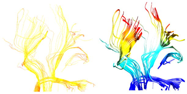
The images were isotropically resampled at 1 mm3 resolution before applying the white matter tractography algorithm. The second order Runge-Kutta streamline algorithm with tensor deflection [31] was used. The trajectories were initiated at the center of the seed voxels and were terminated if they either reached regions with the factional anisotropy (FA) value smaller then 0.15 or if the angle between two consecutive steps along the trajectory was larger than π/4. Each tract consists of 105 ± 54 control points as shown in Figure 1. The distance between control points is 1mm. Whole brain tracts are stored as a binary file of about 600MB in size. Whole brain white matter tracts for 74 subjects are further aligned using the affine registration [26] of FA-maps to the average FA-map.
Figure 1.
Left: control points (red) are obtained from the second order Runge-Kutta streamline algorithm. Subsampled 500 tracts with length larger than 50mm are only shown here. Yellow lines are line segments connecting connecting control points. Right: 19 degree cosine series representation of tracts.
Cosine Series Representation
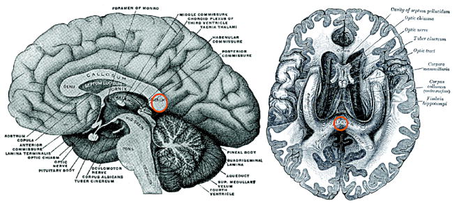
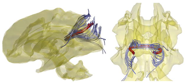
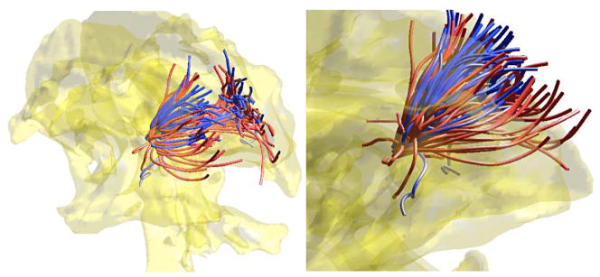
The splenium of the corpus callosum was manually masked by J.E. Lee [32]. See Figure 5 for the location of the splenium in the brain. Then the white matter tracts passing through a ball of radius 5mm at the spleninum are identified. Each subject has 1,943 ± 1, 148 number of tracts passing through the ball. The cosine series representation was constructed for each tract and resulted in 60 coefficients for characterizing the single tract. The within-subject tract averaging was easily done within our representations by averaging the coefficients of the same degree (Figure 6). Figure 7 shows the 74 average within-subject tracts color coded according to autism (red) and controls (blue). We are interested in testing the fiber shape difference between the groups.
Figure 5.
The splenium of the corpus callosum (marked in orange circle) was manually masked and a streamline based tractography algorithm was applied to obtain white matter tracts passing through the splenium. The anatomic drawings are from the wikipedia version of Gray’s Anatomy [22].
Figure 6.
The average tract (red) of 2,149 fibers (blue) in a single subject. 2,149 fiber tracts are subsampled to show few selective tracts. The average tract is obtained by averaging the coefficients of all 2,149 cosine representations. The glass brain is obtained from the average fractional anisotropy map.
Figure 7.
Each streamtube is the average tract in a subject. White matter fibers in controls (blue) are more clustered together with smaller spreading compared to autism (red).
4.2 Results
We have investigated the utility of the proposed parametric representation in discriminating the different populations (42 autistic vs. 32 control subjects) using two different tests.
Two sample T-test
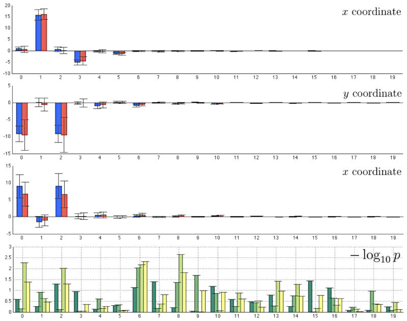
The average tracts for all 74 subjects were obtained using the cosine series representation. The coefficients of the representation are used to discriminate the groups. The bar plots of all 20 coefficients for 3 coordinates are given in Figure 8. The significance of the mean coefficient difference for each degree is determined using the two sample T-test with unequal variance assumption. The corresponding p-value in −log10 scale is given in also given. The first three bars (green to light green) in each degree correspond to the p-values for three coordinates. The minimum p-values are 0.0362 (x coordinate, degree 15), 0.0093 (y coordinate, degree 6) and 0.0023 (z coordinate, degree 8). Note that at least 4 coefficients (degree 0, 2, 6, 8) for the z coordinate show p-value smaller than 0.01. The Bonferroni correction was used to determine the overall significance across different degrees, we have used The T-statistics across different degrees. The Bonferroni corrected p-value for the 8-th degree coefficient of the z coordinate (by multiplying 20 to 0.0023) is 0.0456 indicating that there is significant group difference at the particular spatial frequency. Note that from (5), the 8-th degree corresponds to the spatial frequency of 4.
Figure 8.
Bar plots of coefficients for autistic (red) and control (blue) groups. Each row corresponds to the x, y and z coordinates. The error bars are one standard deviation in each direction. The autistic subjects show larger variability compared to controls, which is consistent with literature [12]. The last row is the p-value plots in −log10 scale. The p-values of the two sample T-test corresponding to x, y and z coordinates are given in three bars (green to light green). The last bar (yellow) shows the p-values of the Hotelling’s T-square test on coefficient vectors.
Hotelling’s T-square test
The problem of using T -test is that the inference has to be done for each coordinate separately. Although T -test gives additional localized information (about z coordinate values being responsible for shape difference), it is not really a clear cut conclusion so we require an overall measure of significance across different coordinates. Therefore, to avoid using T -test separately for each coordinate, we use the Hotelling’s T -square statistic on the vector of 3 coefficients at each degree. The last bar (yellow) in the −log10 p plot shows the resulting p-values. These p-values should be interpreted as the measure of overall significance of three p-values obtained from the T -tests. The minimum p-value is 0.0047 at degree 6. After the Bonferroni correction by multiplying 20, we obtain the corrected p-value of 0.0939, which would be still considered as significant at α = 0.1 level test.
4.3 Simulation
We have performed a simulation study to determine if the proposed framework can detect small tract shape difference between two simulated samples of curves. Our simulations demonstrate the proposed cosine series representation works as expected.
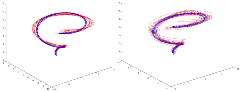
Taking the parametric curve
| (18) |
as a base for simulation, we have generated two groups of random curves. This gives a shape of a spiral with increasing radius along the z-axis. The first group (red curves in Figure 9) consists of 20 curves generated by
Figure 9.
Simulated curves obtained from perturbing the basic curve shape (x, y, z) = (s sin s, s cos s, s), s ∈ [0, 10]. The first figure shows clear group separation while the second figure has too much overlap. We expect the cosine series representation to work extremely well for the first simulation while it may not work for the second simulation.
The second group (blue curves in Figure 9) consists of 20 curves generated by
The non-additive noise is given to perturb (18) a little bit while to make our procedure blind to the underlying additive noise assumption (7). We have performed two different simulations with a different amount of noise variability.
Simulation 1
e1, e2, e3 ~ N (0, 0.12), e4, e5 ~ N (0, 0.22). The p-values are all less than 0.00000243 for Hotelling’s T-square test. The corrected p-value after the Bonferroni correction is less than 0.00005 indicating very strong discrimination between the groups for every degree used. This is evident from the first figure in Figure 9, where we clearly see group separation.
Simulation 2
In the second simulation, we have increased the noise variability such that e1, e2, e3 ~ N (0, 0.22) e4, e5 ~ N (0, 0.52). The smallest p-values is 0.0147. After correcting for multiple comparisons, we obtained the corrected p-value of 0.294 indicating weak group separation in almost all degrees used. The second figure in Figure 9 does not show any clear group separation between the groups.
5. DISCUSSION
We have presented a unified parametric model building technique for a bundle of 3D curves, and applied the method in discriminating the shape of white matter fibers passing through the splenium in autistic subjects. In this section, we discuss two major limitations of the cosine series representation.
Similarly shaped tracts
The cosine series representation assumes the correspondence of two end points of all fiber tracts. In practice, such assumption is not realistic. A short fiber may correspond to a segment of a longer fiber. In this case, the proposed method does not work properly. However, this is not the major limitation in our seed-based fiber tract modeling since it is guaranteed that two end points of all fiber tracts have to match. Also the tracts that pass through the splenium of the corpus callousm are somewhat similar in shape and length (Figure 7). Therefore, we do not need to worry about the case of matching a short tract to a longer tract. We are basically matching tracts of similar shape and length in this study.
Gibbs phenomenon
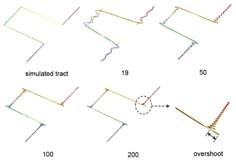
Gibbs phenomenon (ringing artifacts) often arises in Fourier series expansion of discontinuous data. It is named after American physicist Josiah Willard Gibbs. In representing a piecewise continuously differentiable data using the Fourier series, the overshoot of the series happens at a jump discontinuity (Figure 10). The overshoot does not decrease as the number of terms increases in the series expansion, and it converges to a finite limit called the Gibbs constant. The Gibbs phenomenon was first observed by Henry Willbraham in 1848 [44] but it did not attract any attention at that time. Josiah Willard Gibbs rediscovered the phenomenon in 1898 [20]. Later mathematician Maxime Bocher named it the Gibbs phenomenon and gave a precise mathematical analysis in 1906 [5]. The Gibbs phenomenon associated with spherical harmonics were first observed by Herman Weyl in 1968 [18]. The history and the overview of Gibbs phenomenon can be found in several literature [17, 27].
Figure 10.
The within-subject average tract (red) of 2,149 fibers. 2,149 fiber tracts are subsampled to show few selective tracts (blue). The average tract is obtained by averaging the Fourier coefficients of 2,149 cosine representations.
The Gibbs phenomenon will likely arise in modeling arbitrary shaped curves with possible sharp corners. We have demonstrated the Gibbs phenomenon for a simulated tract with jump discontinuities in the following simulation.
Simulation
We have simulated 300 uniformly sampled control points along the parameterized curve (x, y, z) = (t, 0, t) for t ∈ [1, 100) ∪ [200, 300) and (x, y, z) = (t, 1, t) for t ∈ [200, 300). Figure 10 only shows the part of the curve with jump discontinuities. The control points are fitted with the cosine representation with various degrees. As the degree increases to 200, the representation suffers from the severe ringing artifacts. The overshoot shown in Figure 10 does not disappear even as the degree of expansion goes to infinity. Note that white matter fibers are assumed to be smooth so we will not likely to encounter the Gibbs phenomenon in modeling fibers.
Reduction of Gibbs phenomenon
There are few available techniques for reducing Gibbs phenomenon [6, 21]. Most techniques are variations on some sort of kernel methods. For instance, for the Fejer kernel Kn, it can be shown that
for any, even discontinuous, f ∈
 [−π, π] as n → ∞. It has the effect of smoothing the discontinuous signal f and in turn the convolution will not exhibit the ringing artifacts for a sufficiently large n. Particularly related to Fourier and spherical harmonic descriptors, we have introduced an exponential weighting scheme [10, 11]. By weighting Fourier coefficients with exponentially decaying weights, the series expansion can converge faster and reduce the Gibbs phenomenon significantly.
Instead of the k-th degree expansion (8), we define the weighted Fourier expansion as
| (19) |
for some smoothing parameter σ. Then it can be shown that (19) is the finite series expansion of heat kernel smoothing Kσ * f, where the heat kernel is defined as
The expansion (19) can be further shown to be the finite approximation to the solution of heat diffusion
Since the weighting scheme makes the expansion converges to heat diffusion, the estimation at the jump discontinuity is smoothed out reducing the Gibbs phenomenon.
Acknowledgments
This work was supported by NIH Mental Retardation/Developmental Disabilities Research Center (MRD-DRC/Waisman Center), NIMH 62015 (ALA), NIMH MH080826 (JEL) and NICHD HD35476 (University of Utah CPEA). N. Adluru is supported by Computational Informatics in Biology and Medicine (CIBM) program and Morgridge Institute for Research at the University of Wisconsin in Madison.
Contributor Information
Moo K. Chung, Email: mkchung@wisc.edu, Department of Biostatistics and Medical Informatics, Waisman Laboratory for Brain Imaging and Behavior, University of Wisconsin, Madison. Department of Brain and Cognitive Science, Seoul National University, Korea, , url: www.stat.wisc.edu/~mchung
Nagesh Adluru, Email: adluru@wisc.edu, Waisman Laboratory for Brain Imaging and Behavior, University of Wisconsin, Madison.
Jee Eun Lee, Email: jeelee@wisc.edu, Waisman Laboratory for Brain Imaging and Behavior, University of Wisconsin, Madison.
Mariana Lazar, Email: Mariana.Lazar@med.nyu.edu, Center for Biomedical Imaging, School of Medicine, New York University.
Janet E. Lainhart, Email: Janet.Lainhart@hsc.utah.edu, Department of Psychiatry, University of Utah, Salt Lake City
Andrew L. Alexander, Email: alalexander2@wisc.edu, Waisman Laboratory for Brain Imaging and Behavior, University of Wisconsin, Madison
References
- 1.Adler RJ. An Introduction to Continuity, Extrema, and Related Topics for General Gaussian Processes. IMS; Hayward, CA: 1990. [Google Scholar]
- 2.Basser PJ, Mattiello J, LeBihan D. MR diffusion tensor spectroscopy and imaging. Biophys J. 1994;66:259–267. doi: 10.1016/S0006-3495(94)80775-1. [DOI] [PMC free article] [PubMed] [Google Scholar]
- 3.Basser PJ, Pajevic S, Pierpaoli C, Duda J, Aldroubi A. In vivo tractography using dt-mri data. Magnetic Resonance in Medicine. 2000;44:625–632. doi: 10.1002/1522-2594(200010)44:4<625::aid-mrm17>3.0.co;2-o. [DOI] [PubMed] [Google Scholar]
- 4.Batchelor PG, Calamante F, Tournier JD, Atkinson D, Hill DL, Connelly A. Quantification of the shape of fiber tracts. Magnetic Resonance in Medicine. 2006;55:894–903. doi: 10.1002/mrm.20858. [DOI] [PubMed] [Google Scholar]
- 5.Bocher M. Introduction to the theory of Fourier’s series. Ann Math. 1906;7:81–152. [Google Scholar]
- 6.Brezinski C. Extrapolation algorithms for filtering series of functions, and treating the Gibbs phenomenon. Numerical Algorithms. 2004;36:309–329. [Google Scholar]
- 7.Bulow T. Spherical diffusion for 3D surface smoothing. IEEE Transactions on Pattern Analysis and Machine Intelligence. 2004;26:1650–1654. doi: 10.1109/TPAMI.2004.129. [DOI] [PubMed] [Google Scholar]
- 8.Catani M, Howard RJ, Pajevic S, Jones DK. Virtual in vivo interactive dissection of white matter fasciculi in the human brain. neuroimage. NeuroImage. 2002;17:77–94. doi: 10.1006/nimg.2002.1136. [DOI] [PubMed] [Google Scholar]
- 9.Chung MK, Dalton KM, Alexander AL, Davidson RJ. Less white matter concentration in autism: 2D voxel-based morphometry. NeuroImage. 2004;23:242–251. doi: 10.1016/j.neuroimage.2004.04.037. [DOI] [PubMed] [Google Scholar]
- 10.Chung MK, Shen L, Dalton KM, Evans AC, Davidson RJ. Weighted Fourier representation and its application to quantifying the amount of gray matter. IEEE Transactions on Medical Imaging. 2007;26:566–581. doi: 10.1109/TMI.2007.892519. [DOI] [PubMed] [Google Scholar]
- 11.Chung MK, Hartley R, Dalton KM, Davidson RJ. Encoding cortical surface by spherical harmonics. Satistica Sinica. 2008;18:1269–1291. [Google Scholar]
- 12.Chung MK, Robbins S, Davidson RJ, Alexander AL, Dalton KM, Evans AC. Cortical thickness analysis in autism with heat kernel smoothing. NeuroImage. 2005;25:1256–1265. doi: 10.1016/j.neuroimage.2004.12.052. [DOI] [PubMed] [Google Scholar]
- 13.Clayden JD, Storkey AJ, Bastin ME. A probabilistic model-based approach to consistent white matter tract segmentation. IEEE Transactions on Medical Imaging. 2007;11:1555–1561. doi: 10.1109/TMI.2007.905826. [DOI] [PubMed] [Google Scholar]
- 14.Conturo TE, Lori NF, Cull TS, Akbudak E, Snyder AZ, Shimony JS, McKinstry RC, Burton H, Raichle ME. Tracking neuronal fiber pathways in the living human brain. Natl Acad Sci USA. 1999;96 doi: 10.1073/pnas.96.18.10422. [DOI] [PMC free article] [PubMed] [Google Scholar]
- 15.Corouge I, Gouttard S, Gerig G. Towards a shape model of white matter fiber bundles using diffusion tensor MRI. IEEE International Symposium on Biomedical Imaging: Nano to Macro; 2004. pp. 344–347. [Google Scholar]
- 16.Dougherty ER. Random Processes for Image and Signal Processing. IEEE Press; 1999. [Google Scholar]
- 17.Foster J, Richards FB. The Gibbs phenomenon for piecewise-linear approximation. American Mathematical Monthly. 1991;98 [Google Scholar]
- 18.Gelb A. The resolution of the gibbs phenomenon for spherical harmonics. Mathematics of Computation. 1997;66:699–717. [Google Scholar]
- 19.Gerig G, Styner M, Jones D, Weinberger D, Lieberman J. Shape analysis of brain ventricles using spharm. MMBIA. 2001:171–178. [Google Scholar]
- 20.Gibbs JW. Fourieris series. Nature. 1898;59:200. [Google Scholar]
- 21.Gottlieb D, Shu CW. On the Gibbs phenomenon and its resolution. SIAM Review. 1997:644–668. [Google Scholar]
- 22.Gray H. Henry Gray’s Anatomy of the Human Body. 1958 http://en.wikipedia.org/wiki/Splenium.
- 23.Gruen A, Akca D. Least squares 3D surface and curve matching. ISPRS Journal of Photogrammetry and Remote Sensing. 2005;59:151–174. [Google Scholar]
- 24.Gu X, Wang YL, Chan TF, Thompson TM, Yau ST. Genus zero surface conformal mapping and its application to brain surface mapping. IEEE Transactions on Medical Imaging. 2004;23:1–10. doi: 10.1109/TMI.2004.831226. [DOI] [PubMed] [Google Scholar]
- 25.Gueziec A, Pennec X, Ayache N. Medical image registration using geometeric hashing. IEEE Computational Science and Engineering. 1997;4:29–41. [Google Scholar]
- 26.Jenkinson M, Bannister P, Brady M, Smith S. Improved optimization for the robust and accurate linear registration and motion correction of brain images. NeuroImage. 2002;17:825–841. doi: 10.1016/s1053-8119(02)91132-8. [DOI] [PubMed] [Google Scholar]
- 27.Jerri AJ. The Gibbs phenomenon in Fourier analysis, splines and wavelet approximations. Springer; 1998. [Google Scholar]
- 28.Jezzard P, Balaban RS. Correction for geometric distortion in echo planar images from b0 field variations. Magn Reson Med. 2007;34:65–73. doi: 10.1002/mrm.1910340111. [DOI] [PubMed] [Google Scholar]
- 29.Kishon E, Hastie T, Wolfson H. 3d curve matching using splines. Proceedings of the European Conference on Computer Vision; 1990. pp. 589–591. [Google Scholar]
- 30.Kwapien S, Woyczynski WA. Probability and Its Applications. Birkhauser; 1992. Random Series and Stochastic Integrals: Single and Multiple. [Google Scholar]
- 31.Lazar M, Weinstein DM, Tsuruda JS, Hasan KM, Arfanakis K, Meyerand ME, Badie B, Rowley H, Haughton V, Field A, Witwer B, Alexander AL. White matter tractography using tensor deflection. Human Brain Mapping. 2003;18:306–321. doi: 10.1002/hbm.10102. [DOI] [PMC free article] [PubMed] [Google Scholar]
- 32.Lee J, Hsu D, Alexander AL, Lazar M, Bigler D, Lainhart JE. A study of underconnectivity in autism using DTI: W-matrix tractography. Proceedings of ISMRM; 2008. [Google Scholar]
- 33.Leemans A, Sijbers J, De Backer S, Vandervliet E, Parizel P. Multiscale white matter fiber tract coregistration: A new feature-based approach to align diffusion tensor data. Magnetic Resonance in Medicine. 2006;55:1414–1423. doi: 10.1002/mrm.20898. [DOI] [PubMed] [Google Scholar]
- 34.Mori S, Crain BJ, Chacko VP, van Zijl PC. Three-dimensional tracking of axonal projections in the brain by magnetic resonance imaging. Annals of Neurology. 1999;45:256–269. doi: 10.1002/1531-8249(199902)45:2<265::aid-ana21>3.0.co;2-3. [DOI] [PubMed] [Google Scholar]
- 35.Mori S, Kaufmann WE, Davatzikos C, Stieljes, Amodei L, Fredericksen K, Pearlson GD, Melhem ER, Solaiyappan M, Raymond GV, Moser HW, van Zijl PC. Imaging cortical association tracts in the human brain using diffusion-tensor-based axonal tracking. Magnetic Resonance in Medicine. 2002;47:215–223. doi: 10.1002/mrm.10074. [DOI] [PubMed] [Google Scholar]
- 36.O’Donnell LJ, Kubicki M, Shenton ME, Dreusicke MH, Grimson WE, Westin CF. A method for clustering white matter fiber tracts. American Journal of Neuroradiology. 2006;27:1032–1036. [PMC free article] [PubMed] [Google Scholar]
- 37.O’Donnell LJ, Westin CF. Automatic tractography segmentation using a high-dimensional white matter atlas. IEEE Transactions on Medical Imaging. 2007;26:1562–1575. doi: 10.1109/TMI.2007.906785. [DOI] [PubMed] [Google Scholar]
- 38.Persoon E, Fu KS. Shape discrimination using Fourier descriptors. IEEE Transactions on Systems, Man and Cybernetics. 1977;7:170–179. doi: 10.1109/tpami.1986.4767799. [DOI] [PubMed] [Google Scholar]
- 39.Ramsay JO, Silverman BW. Functional Data Analysis. Springer-Verlag; 1997. [Google Scholar]
- 40.Shen L, Chung MK. Large-scale modeling of parametric surfaces using spherical harmonics. Third International Symposium on 3D Data Processing, Visualization and Transmission (3DPVT); 2006. [Google Scholar]
- 41.Shen L, Ford J, Makedon F, Saykin A. surface-based approach for classification of 3d neuroanatomical structures. Intelligent Data Analysis. 2004;8:519–542. [Google Scholar]
- 42.Staib LH, Duncan JS. Boundary finding with parametrically deformable models. IEEE Transactions on Pattern Analysis and Machine Intelligence. 1992;14:1061–1075. [Google Scholar]
- 43.Thottakara P, Lazar M, Johnson SC, Alexander AL. Probabilistic connectivity and segmentation of white matter using tractography and cortical templates. NeuroImage. 2006;29 doi: 10.1016/j.neuroimage.2005.08.051. [DOI] [PubMed] [Google Scholar]
- 44.Wilbraham H. On a certain periodic function. Cambridge and Dublin Math Journal. 1848;3:198–201. [Google Scholar]
- 45.Woods RP, Grafton ST, Holmes CJ, Cherry SR, Mazziotta JC. Automated image registration: I. General methods and intrasubject, intramodality validation. Journal of Computer Assisted Tomography. 1998;22:139. doi: 10.1097/00004728-199801000-00027. [DOI] [PubMed] [Google Scholar]
- 46.Yaglom AM. Correlation Theory of Stationary and Related Random Functions. Basic Results I [Google Scholar]
- 47.Yushkevich PA, Zhang H, Simon TJ, Gee JC. Structure-specific statistical mapping of white matter tracts using the continuous medial representation. IEEE 11th International Conference on Computer Vision (ICCV); 2007. pp. 1–8. [Google Scholar]


