Abstract
Increasing evidence suggests that rare and generally deleterious genetic variants might have strong impact on disease risks of not only Mendelian disease, but also many common diseases. However, identifying such rare variants remains to be challenging, and novel statistical methods and bioinformatic software must be developed. Hence, we have to extensively evaluate various methods under reasonable genetic models. While there are abundant genomic data, they are not most helpful for the evaluation of the methods because the disease mechanism is unknown. Thus, it is imperative that we simulate genomic data that mimic the real data containing rare variants and that enable us to impose a known disease penetrance model. Although resampling simulation methods have shown their advantages in computational efficiency and in preserving important properties such as linkage disequilibrium (LD) and allele frequency, they still have limitations as we demonstrated. We propose an algorithm that combines a regression-based imputation with resampling to simulate genetic data with both rare and common variants. Logistic regression model was employed to fit the relationship between a rare variant and its nearby common variants in the 1000 Genomes Project data and then applied to the real data to fill in one rare variant at a time using the fitted logistic model based on common variants. Individuals then were simulated using the real data with imputed rare variants. We compared our method with existing simulators and demonstrated that our method performed well in retaining the real sample properties, such as LD and minor allele frequency, qualitatively.
Keywords: resampling, logistic regression, simulation, rare SNPs
Introduction
There has been growing evidence that rare and generally deleterious genetic variants have a strong impact on the risks of not only Mendelian diseases, but also many common diseases [Bodmer and Bonilla, 2008; Cirulli and Goldstein, 2010]. This progress in genomic studies of diseases has been made possible by high-throughput sequencing technology. However, identifying such rare variants underlying the diseases remains to be challenging; for example, in the 1000 Genomes pilot project, approximately 15 million single nucleotide polymorphisms (SNPs) were available [1000 Genomes Project Consortium, 2010]. The rare frequencies of the minor alleles (the alleles with less than 50% of the frequency) present additional challenges to the existing methods commonly used in genomewide association studies (GWAS), because the sample sizes are usually not large enough to make inference on the rare variants. Creative algorithms that target on statistical tests on rare variants have emerged [Li and Leal, 2008; Madsen and Browning, 2009; Price et al., 2010; Han and Pan, 2010; Li et al., 2010; Liu and Leal, 2010; Jiang et al., 2011; Brennan et al., 2011]. To further evaluate, refine, and validate the existing methods, simulation data that are realistic are necessary.
Statistical simulations are commonly used to evaluate the performance of statistical models and methods, existing or new. This also is the case when statistical methods and software are developed in genetic studies. When statistical models are clearly defined such as the ordinary linear regression models, the simulation procedures are usually straightforward. However, simulating data in genetic studies can be very challenging due to the complexity of genetic data. We want the simulated datasets to reflect the characteristics of the real datasets, but those characteristics may not be well understood in genetic data. Even though they are well understood, it can be computationally difficult to simulate the data that retain the critical characteristics in the real data. Without simulated data of adequate quality, it is known that a statistical method that performs well on simulated datasets may provide unreliable results on real data [Reich and Patterson, 2005]. For example, in designing a genetic association test statistic that is sensitive to population structures, simulated samples should have the same level of population structure as the real sample to validate the effectiveness of the test statistic. When examining the power of statistical methods, the simulated samples must be realistic enough to challenge the methods in real conditions. In addition to the genetic variations of human populations, other characteristics that are important for simulation include allele frequency and linkage disequilibrium (LD) patterns of genetic markers. The power of a statistical test to detect a risk locus relies heavily on the allelic spectrum (numbers and frequencies of alleles) and on the LD structure around the locus. Specifically, it is desirable for simulated data to possess both local and long range LD patterns and to maintain allele frequencies similar to the real data for which the methods are expected to be applied. Besides the consideration for the genome structure, we need to be aware that complex diseases involve multiple genetic and environmental factors and those factors may interact with each other.
The existing simulation algorithms can be divided into three broad categories [Peng and Amos, 2010]: coalescent [Rosenberg and Nordborg, 2002], forward-time [Peng et al., 2007; Peng and Amos, 2010], and resampling approaches [Wright et al., 2007; Li and Li, 2008]. Coalescent is a model-based simulation method. If the simulation model is not well chosen, the simulated markers can be very different from the real data in terms of allele frequencies, making it difficult to maintain the disease prevalence and ultimately affecting our ability to evaluate the methods. Forward-time approach simulates samples forward in time from an initial population [Peng et al., 2007; Peng and Amos, 2010]. It is known that this approach is computationally intensive; thus, it is inefficient to deal with rare diseases. In addition, the simulation outcomes from this approach are highly sensitive to the initial population because the simulation procedure relies on the evolutionary parameters. Resampling approach starts with real data and avoids the use of an evolutionary process. It has been shown that this method has its advantages in retaining real data properties such as allele frequency and LD [Wright et al., 2007; Li and Li, 2008]. Our approach is in a similar spirit to the resampling approach.
We introduce a regression-based algorithm which imputes rare variants in currently available SNP array data, and performs a resampling approach to simulate samples that contain both common and rare SNPs. We compared the new algorithm with other three simulators, and our results suggest that our algorithm performs well in maintaining realistic sample properties, such as minor allele frequency (MAF) and LD. We implemented our regression-based method in software simuRare, distributed under a GPL license.
Methods
Currently, most of the existing datasets contain only common variants. Hence, generating or imputing rare variants is critical to the development and assessment of methods and software for analyzing rare variants. In what follows, we describe how to simulate genomic data with both common and rare variants. We begin with datasets A and B. The dataset A such as the 1000 Genomes Project data contains both common and rare variants. The dataset B may or may not contain rare variants, but in our simulation, we use only the common variants in dataset B. Clearly, dataset A could serve both roles.
We start with learning the relationship between rare and common variants from dataset A. This relation is then used to impute the rare variants in dataset B, giving rise to an expanded dataset C. Then we perform a resampling method to simulate new samples from dataset C that contains real common variants and imputed rare variants. When building the rare variant models, logistic regression is fitted. After resampling the common and rare variants, disease status can be assigned on the basis of any penetrance model coupled with the contribution of environmental variables.
Simulating Rare Variants from the 1000 Genomes Project
Using the 1000 Genomes Project data as dataset A, we first fit a logistic model for each rare variant against common SNPs that appear in both datasets A and B. For locus r with a rare variant in dataset A, we construct
where pr is the probability of a subject to have the rare allele at the locus in his or her genotype, β0 is the intercept, and βk is the coefficient corresponding to the genotype xrk (coded as 0, 1, and 2 for the number of minor alleles possessed) of the kth locus with a common variant surrounding locus r. For computational reasons, we need to be careful in selecting the common variants as we present below.
For each rare variant, we calculate its correlations with surrounding common variants whose MAFs are greater than 0.01 which is a commonly used threshold for separating common and rare variants, and we selected 20 loci with the largest correlations as the candidate predictors in the logistic model. Then, we start with one locus with a common variant, and add another locus with a common variant at a time, and calculate the model deviance as we move forward with the step-wised models. We choose the model that gives the smallest model deviance as the final logistic model for locus r. We repeat this procedure for each rare variant that we intend to impute.
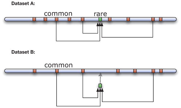
After the regression model is built for each of the rare variants, we use the fitted model to compute the probability of the rare variant based on which we impute the rare variants in dataset B. Furthermore, we can use the MAF in dataset A to separate genotype 1 from genotype 2. Figure 1 presents a schematic diagram of the imputation.
Figure 1. Simulating rare variants using datasets A and B.
For a rare variant, a logistic regression model was built in dataset A using selected common variants surrounding, and this rare variant is then imputed in dataset B based on the constructed logistic model.
Simulating Samples with Realistic Characteristics
For clarity, we call the expanded dataset with imputed rare variants from dataset B as dataset C. The next step is to use dataset C as an initial population to simulate genomic data that contain both common and rare variants and that retain the key characteristics of the real data.
Let Vi = (Vi1, Vi2, …, ViK ) be one of the two haplotypes of individual i, where Vik (k = 1, …, K) is the allele of individual i at locus k in a total of K loci. We first select two individuals a and b who are the most similar in their genomes from the initial population. The similarity is defined as the Pearson correlation between two haplotype vectors Va and Vb. Let Va′ and Vb′ be the other haplotypes of individuals a and b. Then we generate an individual by simulating one haplotype from Va and Va′ and the second haplotype from from Vb and Vb′. We allow cross-overs between Va and Va′ as well as between Vb and Vb′. For each individual, two adjacent loci are sampled from the same haplotype vector with probability (1 + πd)/2, where π(< 1) is a tuning parameter and d is the distance between the two loci in kilobase. After examining both the results from simulated samples and the cross-over patterns in HapMap II CEU data, we found π = 0.99 to be a reasonable choice. Hence we use π = 0.99 as the default value in our current program.
For the convenience of computation in identifying the two highest correlated pairs at any time, we sort all individual haplotype vectors and construct a haplotype matrix, G, such that the summation of correlations of two consecutive rows is maximized. The first row of G is the haplotype vector which has the highest summation of correlations with all other haplotype vectors. Without loss of generality, let V1 be the first row of G. The second row of G is the Vi that has the highest correlation with the first row of G. Likewise, we select the successive rows of G to maximize the correlation with the current row of G.
To generate a simulated individual from dataset C, we randomly select a haplotype vector Gi from G. The other haplotype of individual i is also located and retrieved. Then, another individual i + 1 who has the highest correlated haplotype vector can be located by Gi+1 assuming Gi and Gi+1 are from different individuals. A new individual is simulated by crossing over a pair of haplotypes from individual i and a pair of haplotypes from individual i + 1 at the rate described above; See Figure 2 for a schematic illustration.
Figure 2. Simulating a genotype vector from two individuals (four haplotype vectors).
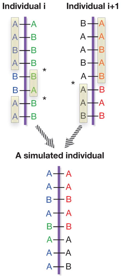
Started with the genomic data of individuals i and i + 1, a new individual is simulated by crossing over a pair of haplotypes from individual i, and a pair of haplotypes from individual i + 1. An asterisk * in the figure indicates the location where a cross-over event occurs. The alleles in the rectangles are selected to form the new individual.
Simulation of Disease Status
To assign the disease status of a simulated individual i, we may calculate the probability of being affected using a logistic regression model, given the disease prevalence and odds ratios at disease loci. For instance, using the following model
where P stands for prevalence, OR1 and OR2 are the odds ratios for SNPs 1 and 2, and OR12 is the odds ratio for the interaction between the two SNPs, we are able to obtain the probability of i being a case (pi) and to use this probability to assign the affection status of the simulated individual.
Results
To examine the performance of our regression-based algorithm and to compare with other existing methods, we applied our algorithm and the other three simulators, including GWAsimulator, simuGWAS, and HAPGEN2 on the HapMap II CEU data as well as the 1000 Genomes chromosome 22 data. GWAsimulator, a resampling method, uses a moving window approach, where haplotypes in each window are simulated according to allele frequency and LD information captured from haplotypes in the HapMap dataset [Li and Li, 2008]. simuGWAS was developed in simuPOP, which is a forward-time simulation environment [Peng and Kimmel, 2005; Peng and Amos, 2010]. Forward-time simulation starts from an initial population and follows its evolution generation by generation, subject to a certain number of genetic or demographic changes [Peng and Amos, 2010]. HAPGEN2 employs the same approach as its previous version HAPGEN which uses an estimate of the fine-scale recombination rate map to simulate haplotypes conditional on the reference haplotype data (HapMap or 1000 Genomes) [Marchini et al., 2007; Spencer et al., 2009; Su et al., 2011]. Instead of using a direct resampling approach, HAPGEN assumes a Hidden Markov Model (HMM) and treats the recombination rates and mutation rates as transition probabilities and emission probabilities, respectively [Li and Stephens, 2003; Marchini et al., 2007; Spencer et al., 2009]. In our first set of simulations, 60 HapMap II CEU founders were employed as a base population. We first performed the rare variant imputation in the base population, and used the generated population with both common and rare SNPs as the initial population for all algorithms. A total of 2000 individuals were simulated in each simulator. We selected a subset of 10,000 consecutive SNPs for the individual simulation after the rare variant imputation. To further compare our simulation method with HAPGEN2, we pursued another set of simulations using the 1000 Genomes Project phase I interim haplotype data download from IMPUTE2 website [Howie et al., 2009]. This dataset contains 1,094 individuals from African, Asian, European, and the American populations. We extracted 75,465 SNPs that cover chromosome 22 using a SNP set obtained from the 1000 Genomes pilot data. 1,239 SNPs with MAF less than 0.01 were involved in these simulations. Using our algorithm and HAPGEN2, we simulated data from the mixed population with 1,094 individuals. In addition, we simulated data from a subset of 87 CEU individuals from the 1000 Genomes data. No disease model was involved in all the simulations. LD and MAF patterns were obtained and compared to the initial population.
LD Patterns
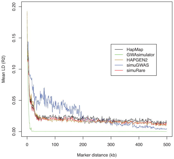
To compare LD patterns between the simulated and the initial population datasets (HapMap and 1000 Genomes), we calculated pairwise LD values and averaged them according to marker distances. Figure 3 plots such LD (R2) curves for four simulated datasets and their reference - HapMap CEU sample. It is evident that the dataset simulated by GWAsimulator experienced a rapid LD decrease even in the very short range. It failed to maintain both short- and long-range LD. For simuGWAS, since the performance of the forward-time method highly depends on the initial population, and since the HapMap CEU population has a very small sample size (60 founders), the forward-time method might experience a rapid loss of genetic diversity due to the genetic drift. To maintain realistic properties of the initial population, we instantly expanded the HapMap CEU population to 1000 at the first generation using the option provided in simuGWAS program. Form Figure 3, simuGWAS had a higher short-range LD and a slightly lower long-range LD than did the HapMap population. The simulated sample from this simulator supplied a more fluctuant LD pattern than that from the real data. HAPGEN2 and the regression-based method, however, showed very similar LD patterns to real data, and maintained both long- and short-range LD satisfactorily. These two algorithms demonstrated comparable performance in mimicking the LD structure of the HapMap CEU population. In some regions of middle-range LD, the regression-based algorithm yielded closer approximations to the real data than did HAPGEN2.
Figure 3. LD patterns by different simulation methods and their reference (HapMap CEU).
Each curve demonstrates the change of the averaged value over pairwise LD (R2) values along different marker distances for four simulators, and their reference HapMap CEU sample (black). Note that simuRare implements our regression-based resampling approach.
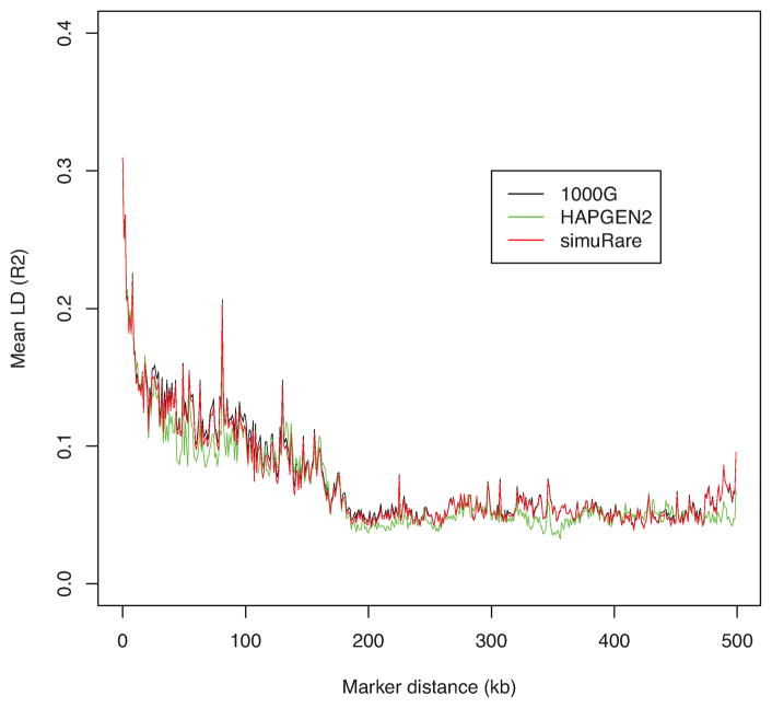
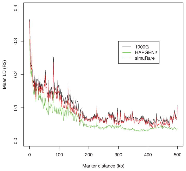
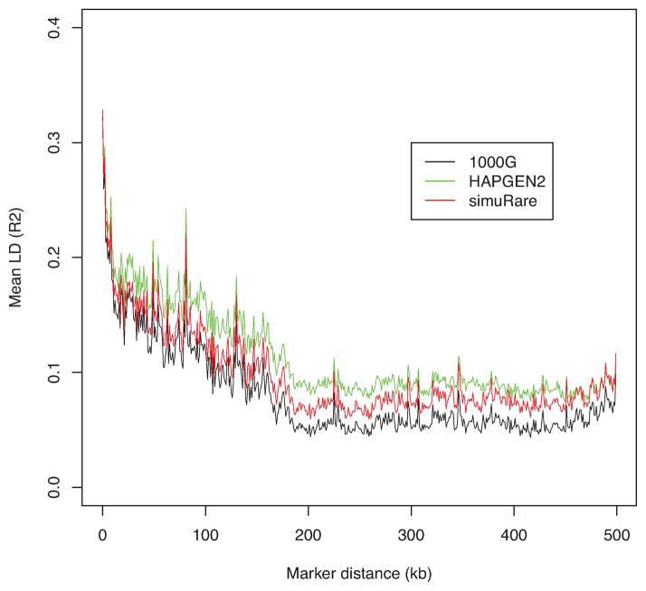
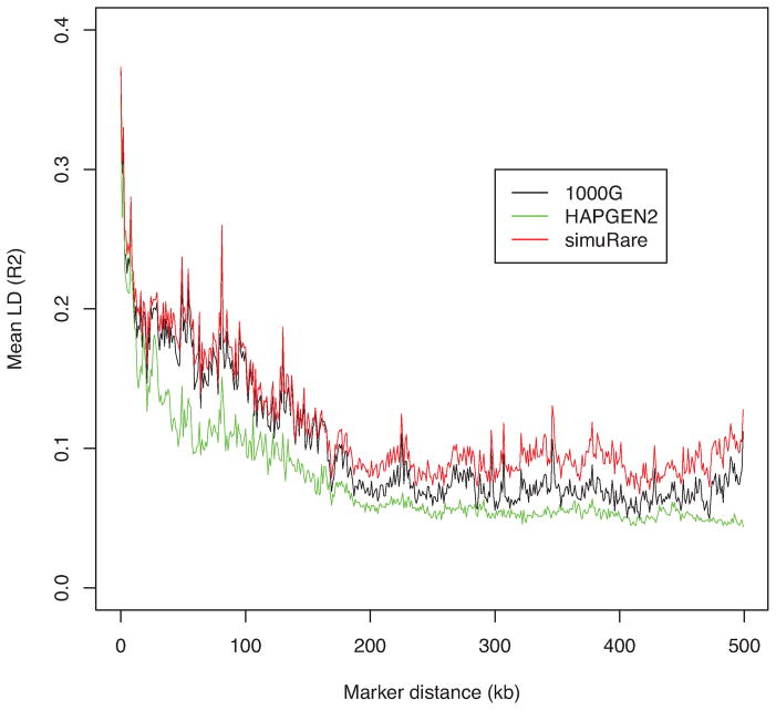
To further investigate the performance and suitable conditions for HAPGEN2 and our regression-based algorithm, we ran another set of simulations using the 1000 Genomes Phase I interim chromosome 22 data on a set with 75,465 SNPs as we described above. We first ran the simulations using the mixed population with 1,094 individuals as the reference data or initial population. Then we took the CEU sample from the reference data, and ran the simulations on the single population consisting of individuals with similar genetic properties. We obtained the LD pattern plots for these two settings as shown in Figures 4 and 6. We then removed SNPs with MAF less than 0.01 and replotted the figures since it has been reported that very low frequency SNPs might lower the average LD values [Goddard et al., 2000]. Figures 5 and 7 show the LD patterns after the rare SNPs were removed.
Figure 4. LD patterns by different simulation methods and their reference (1000 Genomes).
Each curve demonstrates the change of the averaged value over pairwise LD (R2) values along different marker distances for HAPGEN2 and regression-based algorithm, and their reference the 1000 Genomes Phase I interim sample (black).
Figure 6. LD patterns by different simulation methods and their reference (1000 Genomes CEU).
Each curve demonstrates the change of the averaged value over pairwise LD (R2) values along different marker distances for HAPGEN2 and regression-based algorithm, and their reference the 1000 Genomes Phase I interim CEU sample (black).
Figure 5. LD patterns by different simulation methods and their reference (1000 Genomes without rare SNPs).
Each curve demonstrates the change of the averaged value over pairwise LD (R2) values along different marker distances for HAPGEN2 and regression-based algorithm, and their reference 1000 Genomes Phase I interim sample after removing SNPs with MAF less than 0.01 (black).
Figure 7. LD patterns by different simulation methods and their reference (1000 Genomes CEU without rare SNPs).
Each curve demonstrates the change of the averaged value over pairwise LD (R2) values along different marker distances for HAPGEN2 and regression-based algorithm, and their reference the 1000 Genomes Phase I interim CEU sample after removing SNPs with MAF less than 0.01 (black).
From Figure 4 we see that both algorithms produced simulated samples with very similar LD patterns to their reference data. This is especially true for the regression-based method; the LD pattern is almost identical to the 1000 Genomes data. However, the LD curve from HAPGEN2 diverges from the reference curve in both some short- and long- range LD regions. After the rare SNPs are removed, the averaged LD values are increased as displayed in Figure 5. Although both algorithms produced somewhat higher averaged LD values than those from the reference data, the regression-based method imitated the LD structure of the reference data well in the short-range region, and provided closer approximations in the long-range region than those from HAPGEN2. The LD curve from HAPGEN2 is above the curves of simuRare and the 1000 Genomes reference sample. It also has higher variation than simuRare when compared to the curve before the rare SNPs are removed.
When simulating samples on the basis of a single population, as shown in Figures 6 and 7, we noted that our algorithm performed well in keeping the LD structure from the initial population. After deleting the rare SNPs, we found that the averaged LD values from our regression-based algorithm are higher than the reference LD values in the long-range region, but similar in the short-range region. HAPGEN2 did not maintain the LD structure well when using a single population with dense SNPs. When the rare SNPs are removed, however, the LD curve from HAPGEN2 became closer to the reference curve. Nevertheless, its average LD values are still lower than those from the reference data, especially in the short-range region (see Figure 7).
Minor Allele Frequencies
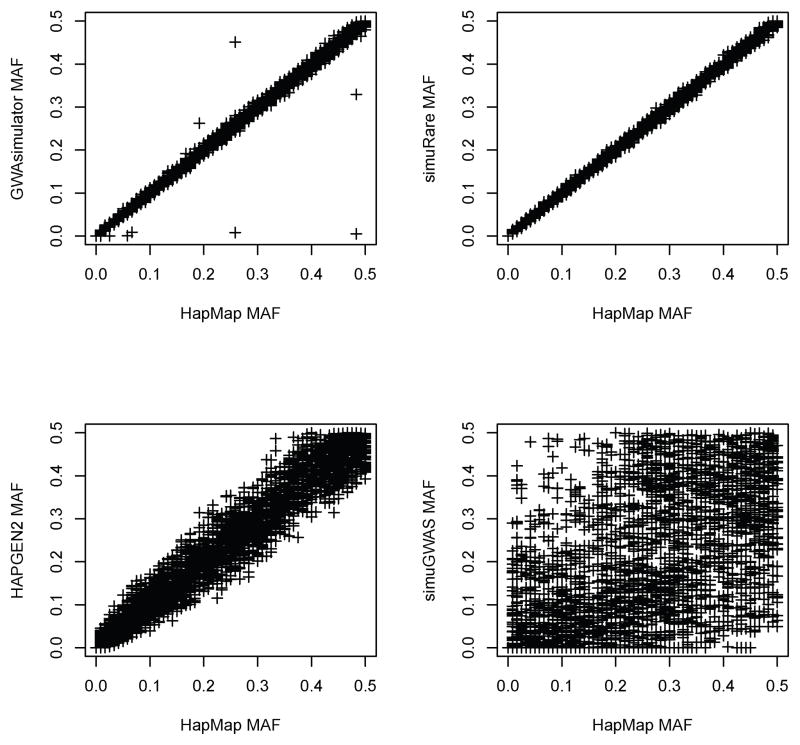
We also compared the MAFs between the simulated datasets and the reference dataset. Figure 8 shows simulated MAFs against HapMap CEU sample with imputed rare SNPs at each locus for the four simulators. GWAsimulator maintained the allele frequencies in most cases, but failed at some loci. Regression-based method provided a strong agreement between simulated data and reference data in terms of MAF. From the lower-left panel in Figure 8, we can observe that many SNPs simulated by HAPGEN2 show inflated or deflated MAFs compared to the reference. In this set of simulations, HAPGEN2 did not maintain MAF very well. To preserve the genetic properties in the simulations, we instantly expanded the HapMap CEU population to 1,000 individuals at the first generation when running simuGWAS. The forward-time algorithm did not maintain the allele frequencies well as can be seen from the lower-right panel in Figure 8. Obviously, expanding the sample size to 1,000 at the beginning of the simulation process is still not enough to preserve the MAF information for the forward-time approach. An even greater sample size may be needed in this situation [Peng and Amos, 2010].
Figure 8. Simulated allele frequencies from four simulators against the reference (HapMap CEU).
Each panel in this figure demonstrates the comparison of the MAFs from one simulator with those from the reference HapMap CEU sample with imputed rare SNPs. Each point represents the deviation of a simulated allele frequency from the real allele frequency obtained from HapMap CEU sample.
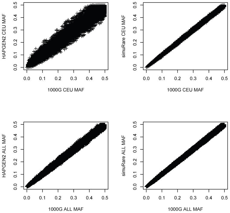
In the simulations that compare HAPGEN2 and simuRare, we obtained similar MAF plots after using the 1000 Genomes CEU population and the mixed population with all individuals as the reference data or initial population. The upper panels of Figure 9 show the MAF patterns when using only the CEU sample to simulate. HAPGEN2 again provided inflated and deflated MAFs in its simulated data, especially for the SNPs with high MAFs. simuRare kept the MAFs of the initial population very well as we showed in the previous example. We calculated the mean square errors (MSEs) as , where pi is the MAF for the i-th SNP and n is the total number of SNPs. For the CEU sample, the MSE from HAPGEN2 is 8.29 × 10⁻⁴, and is 3.16 × 10⁻⁵ from simuRare. The Wilcoxon test shows that the square errors are significantly different (p-value < 2.2 × 10⁻⁶). In the lower panels when all the individuals were involved in the simulations, MAFs form HAPGEN2 simulated sample are more consistent with the MAFs from the reference data, but results from simuRare are still better. The MSEs for the mixed population are 1.08 × 10⁻⁴ and 3.33 × 10⁻⁵ from HAPGEN2 and simuRare, respectively. The Wilcoxon test p-value for the two square errors is again < 2.2 × 10⁻⁶.
Figure 9. Simulated allele frequencies from two simulators against the reference (1000 Genomes).
Each panel in this figure demonstrates the comparison of the MAFs from one simulator with those from the reference 1000 Genomes CEU or mixed population with all individuals from Africa, Asia, Europe, and the Americas. Each point represents the deviation of a simulated allele frequency from the real allele frequency obtained from the 1000 Genomes CEU or mixed sample.
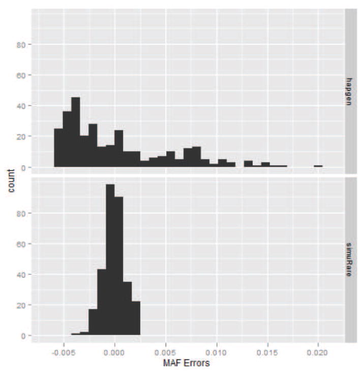
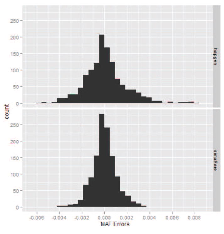
To examine the simulated MAFs for rare SNPs, we extracted the rare SNPs from the simulated and reference data and calculated the MSEs. For the CEU sample, the MSEs are 2.88×10⁻⁵ and 1.10×10⁻⁶ for HAPGEN2 and simuRare, respectively. For the mixed sample, the MSEs are 3.32 × 10⁻⁶ and 1.19 × 10⁻⁶ for HAPGEN2 and simuRare, respectively. The Wicoxon test p-values are < 2.2 × 10⁻⁶ in both cases. Figures 10 and 11 are the histograms for the MAF errors for both algorithms in both cases. Obviously, simuRare shows narrower error distributions than HAPGEN2 in both cases.
Figure 10. Histograms of the simulated MAF errors for the 1000 Genomes CEU sample.
The upper panel is the plot for HAPGEN2, and the lower panel is the plot for simuRare.
Figure 11. Histograms of the simulated MAF errors for the 1000 Genomes mixed sample.
The upper panel is the plot for HAPGEN2, and the lower panel is the plot for simuRare.
Discussion
Through empirical results, we presented the advantages of our approach in maintaining real sample properties, which is important to ensure that the evaluation of new methods is reliable. Specifically, our proposed method retains realistic LD and allele frequency patterns – the most important factors affecting the performance of a gene-mapping method – very well compared to other methods according to our simulation studies. HAPGEN2 employed a HMM rather than direct resampling to avoid the situation that simulated haplotypes are too similar to reference, such as HapMap sample [Marchini et al., 2007]. However, mimicking the real sample properties as close as possible is crucial in investigating the performance of statistical methods in genetic studies. In this report, we used HapMap and the 1000 Genomes data to test our algorithm and to compare the performance of different simulation methods. While our regression-based approach can perform the resampling procedure on any haplotype data, most of the existing methods can only resample from commonly used reference data, such as HapMap and the 1000 Genomes data. In addition, our approach is designed to impute the rare variants from given datasets and maintain the MAFs. To simulate data that are similar to the reference data is important when we develop methodologies to study the etiology of rare variants.
Our resampling method uses a recombination rate that is higher than usual to cross over the two haplotypes of an individual. This approach is similar to the resampling in HapSample which simulates samples by artificially crossing over from a chromosome pool [Wright et al., 2007]. HapSample currently supports resampling from specific reference only which is HapMap Phase I/II data. This limits the use of HapSample.
It is noteworthy that our method is ready for assigning disease status or quantitative traits, even though it is not the purpose of this report. While there have been efforts to simulate rare variants [Proceedings from Genetic Analysis Workshop 17, Boston, MA, USA, 13–16 October 2010, 2011], it is widely known that the existing methods are not convenient to use, and hence it is critical to have an effective alternative, as we proposed here.
We examined our algorithm and HAPGEN2 using different reference data. Our method performed well in all the situations, especially when individuals in the initial population are homogeneous. In some situations, for example after the rare SNPs are removed from plotting the LD curves, our algorithm still kept the LD structures of the reference samples well, especially in the short-range region. HAPGEN2 performed fine in maintaining the LD and MAF structures when using a mixed population in which genetic features may vary in different subpopulations. Nevertheless, its performance is deteriorated when a single population is used. Both LD and MAF patterns are discordant with the reference patterns for HAPGEN2 in this case.
The forward-time simulation approach is flexible in controlling the evolutionary parameters arbitrarily. We are able to simulate very complicated situations using this approach if needed. This approach has its advantages in studying population genetics since it is easy to introduce new genetic features such as natural selection [Peng and Amos, 2010]. However, the datasets simulated in this approach highly rely on the chosen evolutionary parameters and the initial population. To maintain genetic properties, it requires an initial population with a relatively large sample size to start with [Peng and Amos, 2010]. Otherwise, the simulation may lose population information quickly.
Currently, a beta version of the software simuRare can be downloaded from our website http://c2s2.yale.edu/software. The core simulation programs were developed using C language, and a Python interface was created for users to run the software. We continue to improve the user interface and plan to release a much more user friendly version of simuRare in the near future. As a future effort, we believe it would be very useful to generate a large number of replicates of databases with common and rare variants and make them downloadable. These simulated databases could become a benchmark resource for the development and evaluation of methods. As a future project, we plan to use our proposed method to produce such databases and release them at http://c2s2.yale.edu.
Acknowledgments
This work was supported in part by grant R01DA016750 from the National Institute on Drug Abuse and R01GM088566 from the National Institutes of Health. The authors thank Dr. Bo Peng for his support and help on conducting the simulations and on generating the LD plots.
Footnotes
The authors declare no conflict of interest.
References
- 1000 Genomes Project Consortium. A map of human genome variation from population-scale sequencing. Nature. 2010;467(7319):1061–1073. doi: 10.1038/nature09534. [DOI] [PMC free article] [PubMed] [Google Scholar]
- Bodmer W, Bonilla C. Common and rare variants in multifactorial susceptibility to common diseases. Nat Genet. 2008;40(6):695–701. doi: 10.1038/ng.f.136. [DOI] [PMC free article] [PubMed] [Google Scholar]
- Brennan JS, He Y, Calixte R, Nyirabahizi E, Jiang Y, Zhang H. A lasso-based approach to analyzing rare variants in genetic association studies. BMC Proceedings. 2011;5(Suppl 9):S100. doi: 10.1186/1753-6561-5-S9-S100. [DOI] [PMC free article] [PubMed] [Google Scholar]
- Cirulli ET, Goldstein DB. Uncovering the roles of rare variants in common disease through whole-genome sequencing. Nat Rev Genet. 2010;11(6):415–425. doi: 10.1038/nrg2779. [DOI] [PubMed] [Google Scholar]
- Goddard KA, Hopkins PJ, Hall JM, Witte JS. Linkage disequilibrium and allele-frequency distributions for 114 single-nucleotide polymorphisms in five populations. Am J Hum Genet. 2000;66(1):216–234. doi: 10.1086/302727. [DOI] [PMC free article] [PubMed] [Google Scholar]
- Han F, Pan W. A data-adaptive sum test for disease association with multiple common or rare variants. Hum Hered. 2010;70(1):42–54. doi: 10.1159/000288704. [DOI] [PMC free article] [PubMed] [Google Scholar]
- Howie BN, Donnelly P, Marchini J. A flexible and accurate genotype imputation method for the next generation of genome-wide association studies. PLoS Genet. 2009;5(6):e1000529. doi: 10.1371/journal.pgen.1000529. [DOI] [PMC free article] [PubMed] [Google Scholar]
- Jiang Y, Brennan JS, Calixte R, He Y, Nyirabahizi E, Zhang H. Novel tree-based method to generate markers from rare variant data. BMC Proceedings. 2011;5(Suppl 9):S102. doi: 10.1186/1753-6561-5-S9-S102. [DOI] [PMC free article] [PubMed] [Google Scholar]
- Li B, Leal SM. Methods for detecting associations with rare variants for common diseases: application to analysis of sequence data. Am J Hum Genet. 2008;83(3):311–321. doi: 10.1016/j.ajhg.2008.06.024. [DOI] [PMC free article] [PubMed] [Google Scholar]
- Li C, Li M. Gwasimulator: a rapid whole-genome simulation program. Bioinformatics. 2008;24(1):140–142. doi: 10.1093/bioinformatics/btm549. [DOI] [PubMed] [Google Scholar]
- Li N, Stephens M. Modeling linkage disequilibrium and identifying recombination hotspots using single-nucleotide polymorphism data. Genetics. 2003;165(4):2213–2233. doi: 10.1093/genetics/165.4.2213. [DOI] [PMC free article] [PubMed] [Google Scholar]
- Li Y, Byrnes AE, Li M. To identify associations with rare variants, just WHaIT: Weighted Haplotype and Imputation-Based Tests. Am J Hum Genet. 2010;87(5):728–735. doi: 10.1016/j.ajhg.2010.10.014. [DOI] [PMC free article] [PubMed] [Google Scholar]
- Liu DJ, Leal SM. A novel adaptive method for the analysis of next-generation sequencing data to detect complex trait associations with rare variants due to gene main effects and interactions. PLoS Genet. 2010;6(10):e1001156. doi: 10.1371/journal.pgen.1001156. [DOI] [PMC free article] [PubMed] [Google Scholar]
- Madsen BE, Browning SR. A groupwise association test for rare mutations using a weighted sum statistic. PLoS Genet. 2009;5(2):e1000384. doi: 10.1371/journal.pgen.1000384. [DOI] [PMC free article] [PubMed] [Google Scholar]
- Marchini J, Howie B, Myers S, McVean G, Donnelly P. A new multipoint method for genome-wide association studies by imputation of genotypes. Nat Genet. 2007;39(7):906–913. doi: 10.1038/ng2088. [DOI] [PubMed] [Google Scholar]
- Peng B, Amos CI. Forward-time simulation of realistic samples for genome-wide association studies. BMC Bioinformatics. 2010;11:442. doi: 10.1186/1471-2105-11-442. [DOI] [PMC free article] [PubMed] [Google Scholar]
- Peng B, Amos CI, Kimmel M. Forward-time simulations of human populations with complex diseases. PLoS Genet. 2007;3(3):e47. doi: 10.1371/journal.pgen.0030047. [DOI] [PMC free article] [PubMed] [Google Scholar]
- Peng B, Kimmel M. simupop: a forward-time population genetics simulation environment. Bioinformatics. 2005;21(18):3686–3687. doi: 10.1093/bioinformatics/bti584. [DOI] [PubMed] [Google Scholar]
- Price AL, Kryukov GV, de Bakker PIW, Purcell SM, Staples J, Wei LJ, Sunyaev SR. Pooled association tests for rare variants in exon-resequencing studies. Am J Hum Genet. 2010;86(6):832–838. doi: 10.1016/j.ajhg.2010.04.005. [DOI] [PMC free article] [PubMed] [Google Scholar]
- Genetic analysis workshop 17: Unraveling human exome data. BMC Proceedings; Proceedings from Genetic Analysis Workshop 17; Boston, MA, USA. 13–16 October 2010; 2011. [Google Scholar]
- Reich D, Patterson N. Will admixture mapping work to find disease genes? Philos Trans R Soc Lond B Biol Sci. 2005;360(1460):1605–1607. doi: 10.1098/rstb.2005.1691. [DOI] [PMC free article] [PubMed] [Google Scholar]
- Rosenberg NA, Nordborg M. Genealogical trees, coalescent theory and the analysis of genetic polymorphisms. Nat Rev Genet. 2002;3(5):380–390. doi: 10.1038/nrg795. [DOI] [PubMed] [Google Scholar]
- Spencer CCA, Su Z, Donnelly P, Marchini J. Designing genome-wide association studies: sample size, power, imputation, and the choice of genotyping chip. PLoS Genet. 2009;5(5):e1000477. doi: 10.1371/journal.pgen.1000477. [DOI] [PMC free article] [PubMed] [Google Scholar]
- Su Z, Marchini J, Donnelly P. Hapgen2: simulation of multiple disease snps. Bioinformatics. 2011;27(16):2304–2305. doi: 10.1093/bioinformatics/btr341. [DOI] [PMC free article] [PubMed] [Google Scholar]
- Wright FA, Huang H, Guan X, Gamiel K, Jeffries C, Barry WT, de Villena FPM, Sullivan PF, Wilhelmsen KC, Zou F. Simulating association studies: a data-based resampling method for candidate regions or whole genome scans. Bioinformatics. 2007;23(19):2581–2588. doi: 10.1093/bioinformatics/btm386. [DOI] [PubMed] [Google Scholar]


