Potential confounds in estimating trial-to-trial correlations between neuronal response and behavior using choice probabilities

Abstract

Correlations between trial-to-trial fluctuations in the responses of individual sensory neurons and perceptual reports, commonly quantified with choice probability (CP), have been widely used as an important tool for assessing the contributions of neurons to behavior. These correlations are usually weak and often require a large number of trials for a reliable estimate. Therefore, working with measures such as CP warrants care in data analysis as well as rigorous controls during data collection. Here we identify potential confounds that can arise in data analysis and lead to biased estimates of CP, and suggest methods to avoid the bias. In particular, we show that the common practice of combining neuronal responses across different stimulus conditions with z-score normalization can result in an underestimation of CP when the ratio of the numbers of trials for the two behavioral response categories differs across the stimulus conditions. We also discuss the effects of using variable time intervals for quantifying neuronal response on CP measurements. Finally, we demonstrate that serious artifacts can arise in reaction time tasks that use varying measurement intervals if the mean neuronal response and mean behavioral performance vary over time within trials. To emphasize the importance of addressing these concerns in neurophysiological data, we present a set of data collected from V1 cells in macaque monkeys while the animals performed a detection task.

physical stimuli are decomposed into elementary components in the sensory epithelia and subsequently analyzed so that behaviorally relevant information about the external world is represented in central brain areas. Many studies have focused on how sensory information is encoded in the activity of neurons—for example, how the orientation of a visual stimulus is encoded in the spiking activity of a population of neurons in visual cerebral cortex. The inverse question, i.e., how information is extracted from the activity of neurons to give rise to perception or guide behavior, is a fundamental problem that has attracted much attention recently.

Effort has been directed toward understanding whether and how the activity of a given population of neurons contributes to particular perceptual tasks. Correlations between trial-to-trial fluctuations in the responses of individual sensory neurons to a given stimulus and psychophysical performance involving the same stimulus have been a valuable tool for probing this linkage (Nienborg and Cumming 2010; Parker and Newsome 1998). This trial-to-trial correlation, commonly quantified as choice probability (CP) in a discrimination task or detect probability (DP) in a detection task, has been investigated extensively in many brain areas involving different sensory modalities and with various behavioral tasks and is often interpreted as the degree to which the response of a neuron contributes directly to the behavior of interest.

The CP measure (we use CP to refer to both choice probability and detect probability except when they need be differentiated) depends on the considerable variability in the response of a sensory neuron to repeated presentations of a fixed stimulus (Tolhurst et al. 1983). This variability cannot be attributed to adaptation or other known time-related processes and therefore is considered as noise. The noisiness of neuronal responses can be used to link the activity of a given neuron to behavioral reports. If a behavioral report relies on signals from a given neuron, then that report should covary to some extent with the fluctuations in the neuron's activity. For example, if a subject is attempting to detect a weak stimulus using the response of a neuron driven by the stimulus, that subject should be more likely to report seeing that stimulus on those trials when the neuron fires more action potentials.

CP is usually expressed as the area under a receiver-operating characteristic (ROC) function (Britten et al. 1996; Celebrini and Newsome 1994). A value of 1.0 (or 0.0) signifies that the response of a neuron unambiguously predicts perceptual reports on a trial-by-trial basis, and a value of 0.5 signifies that a neuron conveys no information about the perceptual report. CPs for individual sensory neurons are typically small, and average CPs seldom exceed 0.6 in sensory cortical areas (Britten et al. 1996; Nienborg and Cumming 2006; Uka et al. 2005; Williams et al. 2003; but see Dodd et al. 2001 and Palmer et al. 2007). Weak CPs are consistent with the idea that behavioral reports depend on the activity of many neurons, such that no single sensory neuron is strongly correlated with the report (Shadlen et al. 1996).

It is critical that the stimulus used for a CP measurement does not change between different presentations. If, for example, the stimulus intensity changed appreciably from trial to trial, neuronal responses and behavioral performance would covary across trials, creating an artifactual CP greater than 0.5 for reasons that depended only on changes in the stimulus. It is only when the stimulus is constant and behavior follows the noisiness of the neuronal response that CP measurements can provide insights into the neuronal basis of behavior. Of course, even with the most rigorous stimulus control, it is impossible to keep the stimulus condition completely constant between trials. For example, uncontrolled eye movements between trials can lead to subtle yet important differences in neuronal responses and behavior (Herrington et al. 2009).

The small magnitude of CP measures and the potential for artifactual correlations with behavior require that care be taken not only during data collection but also in data analysis. Here we identify potential confounds that can arise in data analysis and lead to biased estimates of CP. In particular, combining neuronal responses across different stimulus conditions or neurons by converting neuronal responses into z scores, a practice common in the literature (Bosking and Maunsell 2011; Heuer and Britten 2004; Nienborg and Cumming 2006; Palmer et al. 2007; Sasaki and Uka 2009; Uka and DeAngelis 2004), can result in an underestimation of CP when the numbers of trials for the two behavioral choices are unbalanced across the pooled data sets. We also demonstrate with neurophysiological data that potential artifacts can arise when the mean neuronal response and mean behavioral performance vary over time within trials in a reaction time task. Methods to avoid these confounds are suggested.

MATERIALS AND METHODS

Simulations.

All simulations and data analyses presented in this study were done with MATLAB (MathWorks). The procedures for the simulations are described in RESULTS. Here we provide details not presented in RESULTS.

The area under the ROC curve (aROC) for a pair of normal distributions having equal variance can be expressed by the following equation (Macmillan and Creelman 2005):

$$\text{aROC}=F\left(d\prime /\sqrt{2}\right)$$ (1)

where F is the cumulative normal probability density function and d′ (d-prime) is defined as

$$d\prime =\frac{{\mu }_2-{\mu }_1}{\sigma }$$ (2)

in which μ₁ and μ₂ are the means of the two normal distributions and σ is their common standard deviation. These equations were used to calculate the population CPs for normal distributions shown in Fig. 1B, top 3 rows, and the simulation presented in Fig. 1C.

Fig. 1.

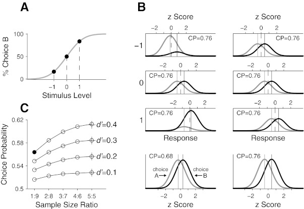
Potential confound in estimation of choice probability (CP) caused by pooling z-scored neuronal responses across different stimulus conditions. A: a hypothetical psychometric function relating the proportion of 1 of 2 choice behaviors in a 2-alternative forced choice (2AFC) task as a function of stimulus level. The two choices are denoted A and B, and a positive stimulus contains signal that evokes the perceptual state mapped onto choice B. The ratios of choice A against choice B at the 3 stimulus levels (−1, 0, 1) are 5:1, 1:1, and 1:5, respectively. B: distributions of the response of a hypothetical neuron to the stimulus at the 3 different levels in A. Distributions of the response preceding the 2 behavioral choices are plotted separately: gray distributions are for choice A and black distributions for choice B, with their means marked by lines of corresponding colors. Distributions on left are in accordance with the ratios of the 2 behavioral choices following the psychometric function in A, and those on right have an equal number of trials for the 2 choices. Top horizontal axis at each stimulus level represents the neuronal response in z score, with its mean marked by a dashed line. Bottom: distributions of the z-scored responses combined across the 3 stimulus levels shown above. C: simulated CPs as a function of sample size ratio for different underlying population CPs indicated by crosses.

For the simulation shown in Fig. 1C, the variance of the normal distributions was 1 for all stimulus levels from which simulated neuronal responses were sampled. The means of the normal distributions for one behavioral choice (choice B) were arbitrarily set as 1, 2, and 3 for the three stimulus levels, and those values were subtracted by d′ to obtain the means for the other choice (choice A). The MATLAB functions “randn” and “poissrnd” were used to generate neuronal responses for the simulations shown in Fig. 1C and Fig. 3A, respectively.

Fig. 3.

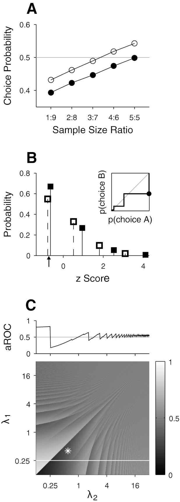
Artifact of combining z-scored neuronal responses across stimulus conditions for a neuron with a low firing rate. A: CPs estimated from simulated responses of a Poisson-spiking neuron firing few spikes. Neuronal responses were combined across 2 stimulus conditions, and the ratio of sample sizes for the 2 behavioral choices was varied (x-axis). Open circles plot the mean CPs simulated under the assumption that the neuronal response was positively correlated with behavior in both stimulus conditions, and filled circles represent the same measurements but under the assumption of no correlation. B: Poisson probability mass functions plotted on a z score axis. Filled squares represent probability masses of a Poisson variable with a mean of 0.4 for events from 0 to 3, and open squares represent the corresponding values for a mean of 0.6. Solid line in inset displays the receiver-operating characteristic (ROC) curve constructed from these probability mass functions assuming that they represent the response distributions for the 2 behavioral choices: the probability mass function with a mean of 0.4 for choice A and the other for choice B. Filled circle in the ROC curve is the point at which the response criterion in the ROC analysis is located between the z scores corresponding to 0 spike count in the 2 distributions (arrow). C: area under the ROC curve (aROC) calculated from pairs of Poisson probability mass functions for different combinations of means (λ₁ and λ₂). Bottom: aROC in gray scale (scale bar on right). Asterisk corresponds to the area under the ROC curve shown in inset of B. Top: aROC when λ₁ was fixed at 0.25 (i.e., cross section of white line, bottom).

Animal preparation and behavioral task.

For the neurophysiological data presented in Figs. 2, 6, and 7, two adult male rhesus monkeys (Macaca mulatta; monkeys 1 and 2; both weighing 11 kg) were used as subjects. All experimental procedures were approved by the Institutional Animal Care and Use Committee of Harvard Medical School. Before training, the monkeys were implanted with a head post and a scleral search coil (Robinson 1963) in one eye for monitoring eye position in an aseptic surgery under general anesthesia. After training was complete for the behavioral task described below, the monkeys underwent a second surgery to implant a stainless steel chamber (19-mm diameter; Crist Instruments) on the skull to allow access of electrodes to the recording areas in primary visual cortex (V1) at an angle of 30° from horizontal in a parasagittal plane.

Fig. 2.

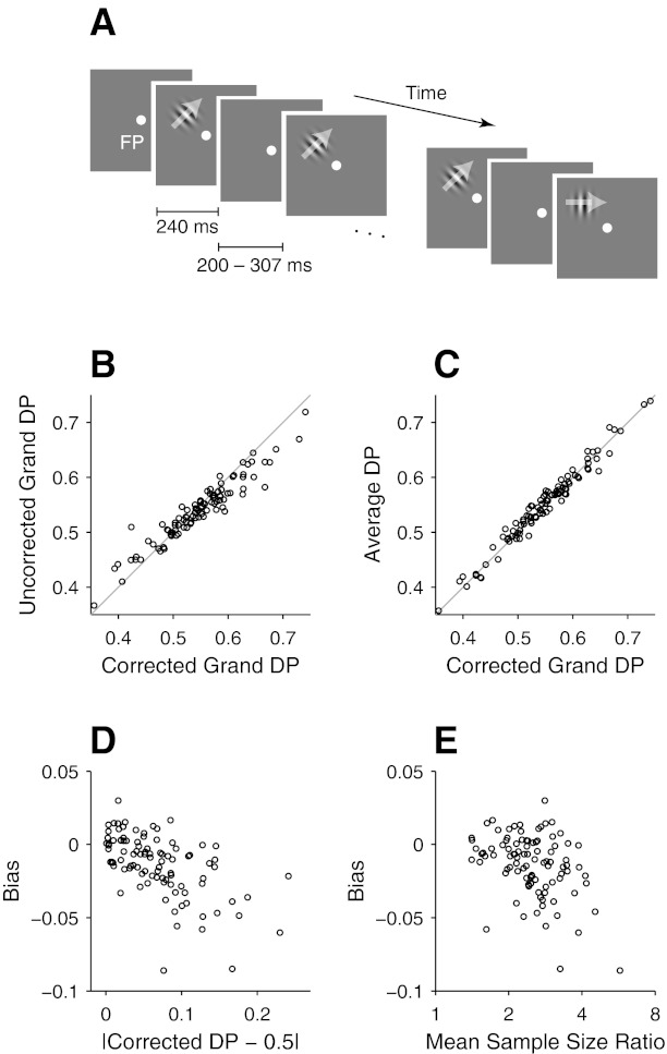
Effects of z-score-based pooling of neuronal responses on detect probability (DP) measures in neurophysiological data. A: schematic representation of the stimulus sequence in a trial of the behavioral task used to collect neuronal data shown in B–E and also in Figs. 6 and 7. See materials and methods for details. FP, fixation point. B: scatterplot between corrected and uncorrected grand DPs of 96 V1 neurons from 2 monkeys. The uncorrected grand DPs (y-axis) were calculated from neuronal responses combined across different target directions with conventional z scores, and the corrected grand DPs (x-axis) were estimated with balanced z-scoring. Gray line is the unity line. C: scatterplot between corrected grand DPs and DPs estimated as the means of DPs calculated with spike counts within individual stimulus conditions (average DP: y-axis). D: scatterplot between the bias of uncorrected grand DPs (y-axis) and the deviation of the corrected grand DPs from 0.5 (x-axis). E: scatterplot between the bias and the mean sample size ratio. See text for the calculation of the mean sample size ratio.

Fig. 6.

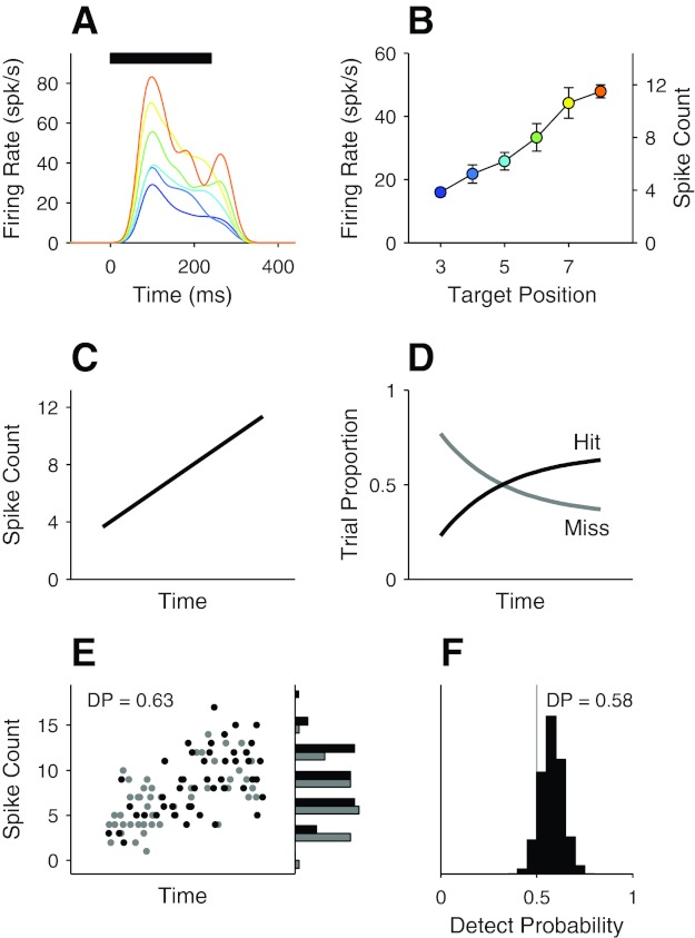
Artifactual DP resulting from concurrent modulations of the neuronal response and the behavioral performance over time within a trial. A: response of 1 of the neurons shown in Fig. 2 to a target stimulus (a 4.2° change from the direction of the reference stimulus). Average responses of the neuron to the target stimulus appearing at different positions in the stimulus sequence within a trial are shown in different colors. Spike trains were convolved with a Gaussian kernel (SD = 20 ms). Horizontal bar indicates time of stimulus presentation. B: mean responses of the neuron in A as a function of target position in the stimulus sequence within a trial. The responses are mean firing rates (or mean spike counts on right y-axis) during a 240-ms interval beginning at 30 ms from the target onset. Colors coding the target position are the same in A and B. Note that the earliest target occurrence in the task was on the 3rd stimulus flash (see materials and methods). Error bars indicate SE. C–F: simulation. C: response profile of hypothetical neuron used in the simulation. The response was modeled after that of the neuron in B. D: hypothetical performance of the subject that was obtained simultaneously with the response of the neuron in C. E: simulated neuronal responses from an iteration of the simulation. Neuronal responses (in spike count) on hit (black circles) and miss (gray circles) trials are plotted on left as a function of the position of the measurement interval within a trial, which was determined by the subject's reaction time, and their marginal distributions on right. See text for details of the simulation procedure. F: distributions of simulated DPs calculated from 2,000 iterations.

Fig. 7.

Physiological data for populations of V1 neurons collected from 2 monkeys (monkey 1, left; monkey 2, right) while the animals performed the same detection task shown in Fig. 2A. A and B: comparisons of the corrected and uncorrected DPs calculated for individual neurons with the corresponding marginal distributions. Only neurons for which at least 10 hit trials and 10 miss trials were available for the calculation of DPs were included, and the mean numbers of trials for a given neuron were 299 for uncorrected and 166 for corrected DPs. See text for details of the methods used to calculate the corrected and uncorrected DPs. C and D: average normalized responses of individual neurons shown in A and B plotted as a function of target position in the stimulus sequence within a trial. The responses for the first 4 of 6 possible target positions are shown because of the scarcity of trials for the last 2 target positions. To obtain normalized responses for a neuron, the mean response within each target position collected at a given target direction was divided by the mean response for that target direction and then averaged across different target directions. E and F: performance as a function of target position. Performance is the average of those from individual sessions in which the neurons in A and B were recorded. For a given session, the proportion correct at a given target position was the number of hit trials divided by the sum of the hit and miss trials, pooled across different target directions that contributed to the calculation of DP of the neuron. Error bars in C–F indicate SE.

After recovery from the first surgery, the monkeys were trained extensively (for 5–6 mo) to perform a direction-change detection task (see Fig. 2A). At the onset of each trial a small white spot (0.1° in diameter) was presented on a CRT display as a fixation point. After the monkey fixated the fixation point for a variable period (375–625 ms), a small drifting Gabor flashed multiple times at the center of the receptive field of the neuron being recorded. Each flash lasted for 240 ms, during which the Gabor drifted in the same direction (reference stimulus), and was followed by a blank screen (200–307 ms). During one pseudorandomly chosen flash the drift direction of the Gabor was different (target stimulus) and the monkey had to make a saccade to the location of the Gabor within 150–600 ms from its onset to get a juice reward. The target stimulus could appear at any flash after the first two flashes, with a probability following an exponential distribution (mean 1,250 ms) truncated at 4,410 ms. The direction of the reference stimulus was set to fall on the flank of the direction tuning curve of the neuron being recorded, and the direction on the target flash changed toward the neuron's preferred direction so that the target stimulus would elicit a stronger response than the reference stimuli. On a given trial, the target direction was pseudorandomly chosen from a set of predetermined values (typically 6) that spanned a range that included the behavioral threshold for detection.

If the animal broke fixation prematurely or failed to respond to the target, the trial ended without reward. Eye positions were sampled at a rate of 500 Hz, and the monkey's fixation behavior was monitored with square electronic windows centered on the fixation point or target location. Each side of the electronic window around the central fixation point was 1.5° or 2°.

Visual stimuli.

Visual stimuli were presented on a gamma-corrected CRT monitor (1,024 × 768-pixel resolution, 75-Hz vertical refresh rate) located 48 cm from the monkey's eye and subtending 43° horizontally and 33° vertically. When recording from neurons with central receptive fields (eccentricities ≤ 3.3°), the monitor was positioned 61 cm from the monkey (35° × 27°) to avoid possible loss of contrast for stimuli of high spatial frequency due to the limited pixel resolution of the monitor (see below for stimulus scaling). In the task, achromatic Gabor functions of the maximum contrast were presented as stimuli on a gray background at a mean luminance of 26 cd/m². The width (standard deviation, SD) and spatial frequency of Gabor functions were scaled according to the receptive field eccentricity with the following formulas:

$$\begin{array}{c}\text{SD}=0.05\times \text{eccentricity}\\ \text{spatial}\text{frequency}=1.5\text{cycles}/\text{SD}\end{array}$$

At each flash, the Gabor function started from an odd-symmetric phase and drifted one full cycle—so the temporal frequency was fixed at 4.2 cycles/s.

Electrophysiological recording and data analysis.

We made extracellular recordings from 96 cells (58 from monkey 1, 38 from monkey 2) in V1. Recordings were made with custom-made platinum-iridium electrodes (Wolbarsht et al. 1960; 0.5–2.5 MΩ at 1 kHz). Signals from the electrode were amplified (BAK Electronics or Plexon), filtered (band pass from 0.5 to 6 kHz) and fed into a time-amplitude window discriminator (BAK Electronics) for isolation of action potentials. The time of each action potential was recorded with a precision of 1 ms. Data were collected mainly from the operculum (receptive field centers ranging from 2.6° to 6.1° eccentricity), but 17 cells were from the calcarine sulcus of monkey 1 (receptive field eccentricities between 17° and 20°).

When a single unit was isolated, before the monkey engaged in the direction-change detection task, the receptive field location was mapped with a computer-generated bar stimulus, and direction tuning was characterized with the same drifting Gabors that were employed in the subsequent behavioral task.

To calculate DPs of individual neurons shown in Fig. 2 and Fig. 7, neuronal responses to the target stimulus were quantified as the number of spikes that occurred during a 150-ms interval beginning 30 ms after stimulus onset. DP was defined as the area under the ROC curve derived from the distributions of the neuronal responses to the target stimulus on hit and miss trials.

RESULTS

In many studies investigating trial-to-trial covariations of neuronal responses with behavior, trials collected in different stimulus conditions are combined to increase statistical power. Sometimes responses from different neurons are combined to estimate the relationship between a population of cells and behavior (so-called grand CP; Britten et al. 1996). In both cases, neuronal responses are first normalized within stimulus conditions or neurons, typically by transforming spike counts into z scores (i.e., subtracting the mean and dividing by the SD). This normalization is essential: without it, a spurious CP will arise because changes in the stimulus can be expected to modulate both neuronal response and behavior.

Combining unbalanced samples can bias choice probability.

Normalizing neuronal responses using z scores to combine results from different stimulus conditions is justified when CPs are independent of stimulus conditions because it will remove stimulus-dependent effects while preserving the rank order of individual observations (Britten et al. 1996). However, caution must be exercised because CP can be underestimated if the ratio of sample sizes for the two behavioral response categories (i.e., two alternative choices in a discrimination task or hit and miss in a detection task) differs appreciably across stimulus conditions for which trials are combined. Figure 1A shows a hypothetical psychometric function describing the probability of one of the binary choices (say A and B) in a two-alternative forced choice (2AFC) task across some adjustment in the stimulus. Suppose one wants to estimate CP from the response of a neuron to stimuli at three different signal levels (−1, 0, 1 in Fig. 1A), which was simultaneously collected with the subject's behavior. Hypothetical distributions of the neuronal response preceding each of the binary behavioral outcomes are shown in Fig. 1B, left, separately for each stimulus level (top 3 rows) and for combined responses after z-score transformation (bottom). In each panel, the distribution of the neuronal response preceding choice A is shown in gray and that preceding choice B in black. The neuron is assumed to respond more strongly to more positive stimulus values: the overall mean of the neuronal response (dashed lines in Fig. 1B) shifts rightward with increasing stimulus value. The neuronal response is modeled as a random variable following a normal distribution having equal variance for all stimulus conditions but a slightly stronger average response on trials when choice B is made. Therefore, the distributions for both behavioral outcomes and all stimulus conditions differ only in their mean and height.

In Fig. 1B, we further assume that at any given stimulus level the response distributions for the two behavioral outcomes are separated by the same amount as measured by d′ (see Eq. 2 for definition). That is, the response of the neuron covaries with the behavioral choice to the same extent regardless of stimulus condition. In this example, d′ is set to 1 in all stimulus levels, which corresponds to a population CP of 0.76 (see Eq. 1). A reasonable prediction, therefore, is that a grand CP based on the combined responses would produce the same CP, but with a smaller confidence interval. However, the combined responses yield a smaller CP (0.68; Fig. 1B, left bottom).

The reduced CP in Fig. 1B can be understood by examining the z-scored response distributions for the different stimulus conditions (top horizontal axes in Fig. 1B, top 3 rows). When the signal was −1, the subject chose A more frequently than B (a ratio of 5 to 1), pulling the overall mean of the z-scored responses (which is zero by definition) toward the mean of the responses on trials in which the subject chose A (see z score axis in Fig. 1B, top left). Consequently, the z-scored response distribution for the dominant choice is closer to a normal distribution centered at a mean of zero. The opposite is true when the signal is 1. Because the dominant behavioral choices differ between the two stimulus conditions but both have z-scored neuronal responses with a mean close to zero, combining the z-scored responses across different stimulus conditions yields response distributions for the two behavioral choices that lie closer together than those in any individual stimulus conditions, effectively diluting the underlying veridical CP (see Fig. 1B, bottom left). The bias will not occur when the ratio of sample sizes for the two behavioral choices is the same across stimulus conditions, for the same reason that converting neuronal responses into z scores would not change CP within stimulus conditions even though the two behavioral choices have unequal numbers of trials. This is illustrated in Fig. 1B, right, for the case when the sample size is always the same for the two behavioral choices (note the different z score assignments in this case).

To measure how unbalanced samples affect CP measurement for a range of imbalances and underlying true CPs, we performed a simple simulation (Fig. 1C). Under the same assumptions made in Fig. 1, A and B, we combined simulated neuronal responses from three different stimulus levels (100 trials at each stimulus level) but varied the ratio of the sample sizes for the two behavioral choices. In Fig. 1C, a ratio of 1:9 means that the numbers of trials for the two behavioral choices at the three stimulus levels were (90, 10), (50, 50), and (10, 90), and a ratio of 3:7 means that they were (70, 30), (50, 50), and (30, 70), and so forth. For each sample ratio, neuronal responses for the two behavioral choices were randomly sampled from normal distributions that were separated by a fixed d′ and converted into to z scores within each stimulus condition. Then a grand CP was calculated from the z-scored responses combined across stimulus levels. This procedure was repeated many times (2,000) for each combination of sample ratio and d′ to generate a pool of synthetic CPs, and their mean was taken as the central tendency for the given sample size ratio and d′.

Figure 1C shows the results of the simulation for five different sample size ratios (from 1:9 to 5:5) and four different d′ values (0.1–0.4). As expected, the underestimation of CP was more profound when the sample sizes for the two behavioral choices were less balanced. The amount of the bias from the unbalanced sample sizes scales with the underlying true CP. Thus appreciable differences may exist for studies that combine responses across a range of behavioral performances, thereby underestimating the true grand CP.

The response of the hypothetical neuron in Fig. 1, B and C, was modeled as a normal random variable. Although spike counts often follow a Poisson distribution, we used normal distributions because the separation between the distributions for the two behavioral choices could be conveniently quantified by d′. However, it should be noted that the confound is not unique to normal distributions. When the mean is reasonably large (e.g., >10; Hodges and Lehmann 1964), a normal distribution is a good approximation to a Poisson distribution and will yield indistinguishable results. When we repeated the simulations shown in Fig. 1C using Poisson random variables with moderate mean spike counts (3–10), the results were virtually identical. We discuss in the following section cases for low spike counts (<3) in which the Poisson distribution departs substantially from the normal distribution.

The bias in the estimation of CP by unbalanced sample size ratios can be avoided in several ways. An obvious solution is to average across CPs estimated for individual stimulus conditions, possibly weighted by the number of trials, instead of combining trials for a grand CP. Another way would be to use a resampling method combined with a bootstrap simulation. For example, within each stimulus condition one can randomly sample the same number of neuronal responses from the two behavioral choices and transform the sampled responses into z scores. The size of the bootstrapped samples within a stimulus condition is set by that of the smaller of the original samples for the two behavioral choices. These z-scored responses are then pooled across different stimulus conditions to construct bootstrap samples for the two behavioral choices, and a bootstrap CP is calculated from the pooled z-scored responses. This procedure is repeated many times, and the mean of the bootstrap CPs thus generated is taken as the estimate for the population CP.

A more efficient way to avoid the underestimation of CP without resorting to a resampling method is to normalize neuronal responses within a stimulus condition as if the samples for the two behavioral choices had an equal number of trials. We note that the mean and variance of the composite of samples from two random variables (in our case, the neuronal responses preceding the two behavioral choices) can be easily derived with a simple algebraic manipulation if the two random variables have well-defined means and variances. Suppose that the sample mean and variance for the two random variables are (x̄₁ and s₁²) and (x̄₂ and s₂²). If the sample sizes of the two variables are n₁ and n₂ correspondingly, then the mean (x̄) and standard deviation (s) of the composite of two samples will be

$$\overline{x}=\frac{n_1{\overline{x}}_1+n_2{\overline{x}}_2}{n_1+n_2}$$ (3)

$$s=\sqrt{\frac{n_1{s}_1^2+n_2{s}_2^2}{n_1+n_2}+\frac{n_1{n}_2{\left({\overline{x}}_1-{\overline{x}}_2\right)}^2}{{\left(n_1+n_2\right)}^2}}$$ (4)

When the sample sizes for the two samples are the same (i.e., n₁ = n₂), they become

$$\overline{x}=\frac{{\overline{x}}_1+{\overline{x}}_2}{2}$$ (5)

$$s=\sqrt{\frac{s_1^2+s_2^2}{2}+\frac{{\left({\overline{x}}_1-{\overline{x}}_2\right)}^2}{4}}$$ (6)

In the general case, the conversion of neuronal responses into z scores will be a linear transformation by using the mean and SD of the composite sample described by Eqs. 3 and 4. The underestimation of CP illustrated in Fig. 1B can be avoided by normalizing neuronal responses within a stimulus condition using the sample mean and SD that are expected when the samples for the two behavioral choices had an equal number of trials (i.e., those described in Eqs. 5 and 6), because it will effectively match the number of trials for the two behavioral choices across different stimulus conditions. We will refer to this method as balanced z-scoring.

To see whether normalizing neuronal responses by balanced z-scoring yields an unbiased estimate of CP and to compare its reliability with that of the other methods, we extended the simulation presented in Fig. 1C. We applied the three methods (arithmetic mean, resampling, and balanced z-scoring) to estimate CP from random samples of hypothetical neuronal responses collected in three different stimulus conditions. The pairs of the sample sizes for the two behavioral choices in three different stimulus conditions were (90, 10), (50, 50), and (10, 90), and in each stimulus condition the population neuronal responses for the two behavioral choices were separated by the same amount (d′ = 0.4). This simulation configuration is the same as that of the point marked by a filled circle in Fig. 1C, in which the combined response using the conventional z scores yielded a CP of 0.56, whereas the true CP was 0.61. When the results of 2,000 iterations were compared, we found that the estimates from all three methods converged on the true CP with comparable confidence intervals. The mean of CPs estimated with balanced z-scoring was 0.61, with the width of a 95% confidence interval being 0.18. The corresponding values were 0.61 and 0.20 for the arithmetic mean of CPs from individual stimulus conditions and 0.61 and 0.17 for the resampling method. The simulation indicates that normalizing neuronal responses with balanced z-scoring corrects for the bias as effectively as the resampling method that is computationally more expensive.

To confirm this bias in neurophysiological data, we present in Fig. 2 a set of data collected from V1 cells in two monkeys while they performed a direction-change detection task (Fig. 2A; see materials and methods for details of the behavioral task). For individual neurons, we estimated DPs in three different ways from counts of the spikes from individual neurons during a 150-ms interval beginning at 30 ms after stimulus onset. For a given neuron, a grand DP was calculated from trials combined across different target directions (typically 4) using conventional z scores (uncorrected grand DP in Fig. 2B). Also, we calculated a grand DP, using balanced z-scoring (corrected grand DP in Fig. 2, B and C). Finally, a DP was estimated as the mean of individual DPs that were calculated with spike counts within individual stimulus conditions (average DP in Fig. 2C). Trials in a given target direction were included only when a minimum of five trials were available for both miss and hit responses and the mean firing rate was higher than 5 spikes/s during the measurement interval (see the following section for the effects of low firing rates on CP measures). With these criteria, there were on average 2.5 times as many trials for one type of behavioral response as the other in a given stimulus condition for a given neuron.

Consistent with the simulations, the uncorrected grand DPs were closer to 0.5 than the corrected grand DPs. That is, the uncorrected grand DPs tended to be below the unity line in Fig. 2B when the corresponding corrected DPs were larger than 0.5 and above the unity line when the corresponding corrected DPs were smaller than 0.5. The means of the uncorrected and corrected grand DPs were 0.540 and 0.547, respectively, and the difference was statistically significant (P = 0.004, t-test for the pairwise difference). On the other hand, the corrected grand DPs did not statistically differ from the means of individual DPs estimated within stimulus conditions (P = 0.19; Fig. 2C), which suggests that the corrected grand DPs were better estimates of the underlying true DPs.

Based on these results, for a given neuron we defined the bias as [uncorrected grand DP − corrected grand DP] but inverted the sign for those neurons that had a corrected grand DP smaller than 0.5. The mean bias was −0.014 and was significantly smaller than zero (P < 10⁻⁸). Next we examined whether this bias depended on the magnitude of DP and the degree of the imbalance of sample size ratios across combined stimulus conditions, as shown by the simulation in Fig. 1C.

To quantify the imbalance of sample size ratios for a given neuron, we took the log of the ratio between the numbers of miss and hit trials for each stimulus condition and averaged the absolute values of these logarithmic sample size ratios across stimulus conditions. Then the mean sample size ratio was calculated as the anti-log of this mean value. The bias was correlated with both the magnitude of the corrected grand DP (r = −0.58, P < 10⁻⁹; Fig. 2D) and the log of the mean sample size ratio (r = −0.39, P < 10⁻⁴; Fig. 2E). The bias had also significant partial correlations with these two variables when the other variable was controlled (r = −0.59, P < 10⁻⁹ with the magnitude of the corrected grand DP; r = −0.41, P < 10⁻⁴ with the log mean sample size ratio).

Low spike counts render choice probability unreliable when estimated using z-scored pooling.

In Fig. 1C the simulated CP appears to converge on 0.5 as the sample size ratios become increasingly unbalanced. Such a result is predicted given the fact that in the limit the combined neuronal responses will have the same normal distribution for both behavioral choices. However, this may not be true when CPs are estimated from a neuron with a low firing rate. Indeed, z-score-based pooling can lead to a grand CP that is opposite from that estimated within individual stimulus conditions. This can happen because neuronal responses quantified with spike counts are discrete and bounded by zero.

To illustrate the problem, we performed a simulation similar to that shown in Fig. 1C. In the simulation, the neuronal response was modeled as a Poisson (rather than normal) random variable and sampled from two stimulus conditions. In one set of simulations, we assumed that the neuronal response did not covary with behavior (i.e., a population CP of 0.5) and set the mean spike count for the two stimulus conditions as 0.4 and 0.6. In another set of simulations, we made simulated neuronal responses to be positively correlated with behavior as in Fig. 1C. For this, we set the mean spike for one behavioral choice 1.25 times higher than that of the other. Thus mean spike counts were 0.4 and 0.5 in one stimulus condition and 0.6 and 0.75 in the other condition. With these mean differences the population CP within stimulus condition will be 0.53 for the first stimulus condition and 0.55 for the second when estimated from an ROC analysis applied to the corresponding probability mass functions. In each iteration, 100 spike counts were generated for each stimulus condition and transformed into conventional z scores. Each spike count was randomly drawn from a Poisson distribution with the mean specified by the behavioral choice and stimulus condition.

Figure 3A plots mean of simulated CPs (2,000 iterations) as a function of sample size ratio. CPs simulated under assumption of positive correlations with behavior are shown by open circles and those simulated under assumption of no correlation are shown by filled circles. As in Fig. 1C, a sample size ratio of 1:9 indicates that the number of trials for the two behavioral choices was (90, 10) in one stimulus condition and (10, 90) in the other. Unexpectedly, CPs simulated under the assumption of no correlation with behavior did not converge on 0.5, but instead decreased monotonically as sample sizes became less balanced. Moreover, CPs simulated for neuronal responses that were positively correlated with behavior were shifted upward by a fixed amount relative to those simulated under the assumption of no correlation. This yielded CPs < 0.5, suggesting a negative correlation with behavior, for samples less balanced than a ratio of 4:6.

To understand this phenomenon, we examined the probability mass function of Poisson variables with means of 0.4 and 0.6 that were used to simulate the neuronal responses under the assumption of a population CP of 0.5 in Fig. 3A. Figure 3B plots probabilities of observing 0–3 spikes in each stimulus condition on a z score axis (i.e., spike counts have the mean subtracted and are divided by the SD; filled squares for a mean spike count of 0.4, open squares for 0.6). Because the mean spike count is low, in both conditions the observed spike counts are most often zero. However, a zero spike count corresponds to different z scores for the two distributions. Importantly, the value will be smaller for a distribution with a larger mean spike count (z = −0.77 vs. −0.63 for a mean spike count of 0.6 and 0.4, respectively). If the behavioral choice that makes up the majority of responses in one stimulus condition differs from the other, the response distributions for the two behavioral choices will resemble the probability mass functions shown in Fig. 3B. In the limit, neuronal responses for one behavioral choice are collected entirely from one probability mass function and those for the other behavioral choice from another probability mass function. The ROC curve in Fig. 3B, inset, was constructed from the probability mass functions plotted in the same figure. It can be seen that aROC is much smaller than 0.5 mainly because one distribution (filled squares in Fig. 3B) lies entirely to the right of a small range of negative values on the z score axis but the other distribution (open squares in Fig. 3B) has most of its points to the left (arrow). This range lies between the points corresponding to zero spike count in the two distributions, which maps onto the point marked with a filled circle on the ROC curve in Fig. 3B, inset.

To explore this artifact in more detail, we applied an ROC analysis to pairs of Poisson probability mass functions plotted on a z score axis as shown in Fig. 3B. Figure 3C, bottom, shows aROC value, with the mean of one distribution on the y-axis (λ₁) and that of the other distribution on the x-axis (λ₂). The asterisk in Fig. 3C corresponds to the area under the ROC curve shown in Fig. 3B, inset. For all pairs of means, Fig. 3C represents the bias in the limit of unbalanced sampling when CP is estimated using z-scored neuronal responses combined across two stimulus conditions given that the true CP is 0.5. In general, the bias is largest when mean spike counts are low: deviation from 0.5 is most prominent in the lower left corner of Fig. 3C. The direction of the bias is contingent on the way the behavioral choice is linked to the selectivity of the neuronal response for the stimulus. Ironically but understandably, for a given mean spike count, the bias is larger for a smaller difference in the mean spike count between the two stimulus conditions. This behavior can be better seen in Fig. 3C, top, which plots aROC when the mean spike count for one stimulus condition is fixed at 0.25, which corresponds to the cross section delineated by the white line in Fig. 3C, bottom. The largest departures from 0.5 occur when the other mean rate approaches 0.25. Interestingly, the aROC in this panel converges slightly above 0.5 when the mean spike count in the other stimulus condition becomes large.

In summary, the artifact illustrated in Fig. 3C demonstrates that combining low spike counts across different stimulus conditions with z-score normalization can result in unreliable CPs. This artifact arises because of the discrete nature of neuronal responses that are bounded by zero, and the fact that distributions of responses are skewed toward infinity for neurons with low firing rates (Fig. 3B). Therefore, combining neuronal responses with z-score normalization should be avoided for neurons with very low mean spike counts.

In the following sections, we discuss the effects of using variable time intervals for measuring neuronal responses on CP estimation as well as potential confounds that can arise because of nonstationarity of neuronal and behavioral responses within a trial. Here we use “nonstationarity” to refer to any systematic temporal modulation of the neuronal response or behavioral performance.

Choice probability depends on length of measurement interval.

In previous studies, trial-to-trial correlations of neuronal activity with behavior have been estimated based on neuronal responses measured for variable time intervals ranging from a few hundred milliseconds to a few seconds. The large variance in the length of the measurement intervals makes it difficult to compare CPs reported in different studies. This is because CP of the same neuron will vary depending on the length of the measurement interval. If the response of a neuron follows Poisson statistics, the signal-to-noise ratio of the response, defined as the ratio of mean to SD of spike count, will increase with the square root of the time during which spikes are counted. This means that response distributions of a neuron for the two behavioral choices, which determine aROC, will be more separated for a longer measurement interval yielding a larger CP, provided that the ratio of responses for the two behavioral choices remains constant. Consider, for example, d′ defined in Eq. 2, which is a measure of the separation between two normal distributions that approximate Poisson distributions when the mean is large. If the measurement interval is doubled, the mean difference (i.e., μ₂ − μ₁) will also double. However, the SD (i.e., σ) will increase only by the square root of 2, yielding a larger d′.

We show in Fig. 4 how CP varies with the length of measurement interval under the assumption of Poisson spiking. Each curve in Fig. 4 represents CP for a pair of Poisson distributions for which the means are of a fixed ratio. For example, the curve denoted by 2% means that the mean spike count for one behavioral choice is higher by 2% than that for the other choice. The x-axis is the mean spike count for the behavioral choice linked to the weaker response. CPs appear to vary with the length of measurement interval in a similar manner regardless of the ratio of neuronal responses between the two behavioral choices, i.e., one curve seems a scaled version of another. However, for a given mean ratio the effect is not insignificant. For example, CP for a mean spike count of 50 was 0.578 (square in Fig. 4) and that for 25 was 0.556 (circle in Fig. 4) when the mean spike count difference in two behavioral choices was 4%. Therefore, halving the measurement interval reduces CP by nearly 30%. This relation between the aROC and length of the measurement interval was previously described in the context of measuring neurometric performance of a neuron distinguishing between two stimuli (Zohary et al. 1990) and supported by physiological data (Britten et al. 1992; Heuer and Britten 2004; Uka and DeAngelis 2003).

Fig. 4.

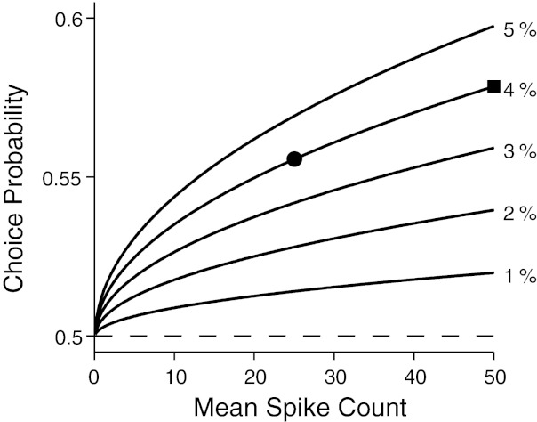
Relationship between length of measurement interval and CP. Length of the measurement interval is represented as the mean spike count during the interval (x-axis) assuming that the mean spike count is proportional to the length of the measurement interval. CP at a point on each curve was numerically calculated by applying an ROC analysis to a pair of Poisson probability mass functions. The mean of one of the probability functions was the value on the x-axis, and the other was higher by the amount indicated at the end of each curve. Horizontal dashed line indicates no correlation between the neuronal response and behavior.

Nonstationary neuronal responses can bias choice probability.

Stimulus-evoked neuronal responses are usually not stationary, and the mean firing rate often varies systematically over time within a trial. In particular, neurons often respond initially with strong transient spiking followed by weaker sustained firing. This type of nonstationarity of spiking activity may not bias the estimation of CP as long as a fixed measurement interval is used and a Poisson-like spiking process can be assumed.

To illustrate this point, Fig. 5, A and B, plot the responses of two hypothetical neurons to an identical stimulus separately for the binary behavioral choices that follow the responses (black and gray lines). The response of the neuron in Fig. 5A is stationary, whereas that in Fig. 5B decreases monotonically over time. However, this difference need not affect CP. At any given time the mean response preceding one behavioral choice (black lines in Fig. 5) is higher by the same amount than that preceding the other (gray lines) for both neurons. Despite the difference in the stationarity of spiking activity, if the overall mean firing rate during the measurement interval (demarcated by gray patches in Fig. 5, A and B) is the same for the two neurons, distributions of the neuronal responses preceding the two behavioral choices will be similar (Fig. 5, A and B, right), and will therefore yield equivalent CP. This is because under the assumption of a Poisson spiking process, the number of spikes within an interval observed for two neurons will conform to the same Poisson distribution as long as the neurons have the same mean spike count during the interval, which is the time integral of the firing rate over the interval (Rieke et al. 1997), regardless of their firing patterns.

Fig. 5.

Effects of nonstationary neuronal responses and variable measurement intervals on CP measurement. A: mean firing rate of a neuron with stationary spiking activity is displayed for 2 behavioral choices (black and gray lines) on left. Gray area indicates the interval for which neuronal responses are quantified to estimate CP. Distributions of neuronal responses for the 2 behavioral choices are shown on right in the corresponding colors with their means indicated by lines. B: response of a neuron with nonstationary spiking activity shown in the same format used in A. C: the same neuron in B to illustrate a situation in which the measurement interval varies in the offset between trials. Gray areas indicate examples of the measurement interval in 2 different trials. Right: distributions of neuronal response quantified by using such measurement intervals whose offset is random and uniformly distributed within a trial. To show the distributions in the limit, the length of the interval is assumed to be infinitesimally small.

On the other hand, if the measurement interval is not fixed, but instead varies between trials, CP estimated from a nonstationary neuron will be generally smaller (i.e., closer to 0.5) than that from a stationary neuron. This can happen if one examines neuronal responses aligned on a certain event, such as the subject's response when that response varies with respect to the onset of the stimulus-evoked neuronal response (as in a reaction time task). For example, gray areas in Fig. 5C, left, show such measurement intervals from two trials applied to the same nonstationary neuron as in Fig. 5B. Combining neuronal responses from different intervals will introduce the variance in the response over time into the distributions of the neuronal response for the two behavioral choices, as shown in Fig. 5C, right. The CP based on these response distributions will be smaller than when it is estimated in the same way from a stationary neuron (note that the response distributions in Fig. 5C are wider than those in Fig. 5A even though the difference in the means for the 2 behavioral choices is the same for the 2 neurons).

Another situation in which a nonstationary response can lead to an underestimation of CP is when the measurement interval varies in length even though the start of the measurement interval is fixed. This procedure can also introduce the variance of neuronal response over time into CP measurements. For example, in a reaction time task, one could measure neuronal responses during an interval that ends at the subject's response (Cohen and Newsome 2009; Palmer et al. 2007). In such a situation, CP is usually estimated from neuronal responses normalized by the length of the measurement interval, i.e., in terms of firing rate instead of spike count. This poses another problem because CP will increase with the length of the interval during which spikes are counted if the spiking activity of the neuron follows Poisson statistics (Fig. 4).

Nonstationary behavior can bias detect probability.

The situation exemplified in Fig. 5 is a consideration whenever the neuronal response is quantified using intervals that vary in either offset or length. The problem is exacerbated in a detection task when the behavioral performance varies over periods during which the neuron may undergo response modulations. Specifically, an artifactual correlation can arise when the detection performance improves or deteriorates depending on the time at which the stimulus appears within a trial. In principle, an artifactual CP could also occur for individual neurons in a discrimination task if the subject's choice behavior becomes increasingly biased or the subject's discrimination improves over time within a trial. However, to introduce an artifactual CP at the population level, such behavioral bias would have to change systematically with the tuning preferences of the recorded neuron (see discussion). Because such confounds are of little concern for typical experimental designs for discrimination tasks, we confine our discussion to the effects of concurrent neuronal and behavioral modulations on DP measurements.

The problem is presented in Fig. 6 for one of the neurons shown in Fig. 2. Figure 6A plots the average response profiles of the neuron to a target stimulus, sorted by the position of the target in the stimulus sequence within a trial (the target position is color-coded in the same way in Fig. 6B). The neuron responded to the same stimulus with different magnitudes depending on where it appeared in the stimulus sequence (Fig. 6B). The response increased monotonically with the temporal position of the stimulus within a trial, which is somewhat surprising because one might expect a weaker response for a later target if the neuronal response was adapted by repeated presentations of the preceding reference stimulus.

As with the CP discussed in Fig. 5, B and C, the DP calculated by combining responses to stimuli at all target positions can be expected to be smaller than the DP calculated within any one target position. But this nonstationary response can have a further effect if behavior is not stationary across target positions in the stimulus sequence. Suppose that the response of this example neuron was unrelated to the monkey's detection behavior on trial-by-trial basis (i.e., DP of 0.5) but the monkey was better at detecting target stimuli presented later in a trial. From this hypothetical situation, which is depicted in Fig. 6, C (neuronal response) and D (behavioral performance), it is not difficult to see that the DP measured from this neuron will be higher than 0.5 because the sample of miss trials will include more trials in which the target appeared earlier (eliciting weaker responses from the neuron) and the sample of hit trials will include more trials in which the target appeared later (eliciting stronger responses from the neurons). This prediction was confirmed by a simple simulation. In the simulation, we allowed the target to occur at any time in a trial with an equal probability. Once the target time was specified for a trial, the neuronal response was randomly drawn from a Poisson distribution with the mean specified by the response function shown in Fig. 6C at the target time, and the trial was randomly tagged as either hit or miss following the subject's performance at the target time (Fig. 6D). Figure 6E plots simulated neuronal responses generated in a single iteration of the simulation. As expected, the response of the neuron on hit trials (black circles) was higher than on miss trials (gray circles; see distributions in Fig. 6E, right), yielding a DP of 0.63, although the neuronal activity had no direct bearing on the behavioral response. Figure 6F shows the distribution of simulated DPs from 2,000 iterations.

One way to alleviate this problem would be to bin trials according to their positions of the measurement interval in time and normalize neuronal responses within individual bins. Such a strategy would be effective if the bin size is sufficiently small. However, this approach may compromise statistical power because trials falling on a bin can be used only when a sufficient number of trials are available for both behavioral outcomes in that bin. For example, if there is only one type of behavioral response in a bin, those trials will be excluded from the analysis. This is expected when the bin size is too small and behavioral performance varies considerably over time within a trial. Therefore, the choice of bin size should be guided by the degree to which neuronal and behavioral responses are modulated and the total number of trials. Nevertheless, the binning procedure is expected to give a less biased estimate of DP.

To emphasize the importance of addressing these issues in neurophysiological data, we further analyzed data shown in Fig. 2 and present the results separately for individual animals in Fig. 7 (monkey 1, Fig. 7, left; monkey 2, Fig. 7, right). Figure 7, A and B, compare DPs of individual neurons that were corrected for the potential confounds discussed in this study (x-axis) with uncorrected DP estimates (y-axis). To correct data for the potential confounds, for a given target direction spike counts were normalized within each target position in the stimulus sequence in a trial with balanced z-scoring: normalization within target positions was to remove the effects of temporal modulations of the neuronal response and behavioral performance within a trial and balanced z-scoring to avoid the artifact due to unbalanced sample sizes. DP was then calculated from the z scores combined across different target positions and different target directions. Trials were included only when a minimum of five trials were available for both miss and hit responses for a given target position. The uncorrected DPs are the same as those plotted on the y-axis in Fig. 2B. It should be noted that, as pointed out previously for the binning procedure, the requirement for the minimum number of trials within target positions in the corrected DP reduced the total number of trials included in the calculation compared with the uncorrected DP (see Fig. 7).

Although the corrected DPs are correlated with the uncorrected DPs for both monkeys, the two animals are distinct: the mean values were virtually identical for the two DP measurements in monkey 1 (P = 0.44; Fig. 7A), whereas they were markedly different in monkey 2 (P = 0.004; Fig. 7B), with the average corrected DP being reduced to chance. That the correction procedure reduced DP in monkey 2 suggests that for this animal both neuronal response and behavioral performance might have varied systematically over time within a trial, because correction for the imbalanced sample sizes (Figs. 1 and 2) or for the nonstationarity of neuronal response (Fig. 5) would only increase the correlation. To verify this possibility, we examined neuronal modulations and behavioral performance as a function of target position in the stimulus sequence within a trial. Consistent with the hypothesis, both the average neuronal response (Fig. 7D) and the average behavioral performance (Fig. 7F) in monkey 2 increased monotonically with the target position. In contrast, the response of the neurons in monkey 1 decreased slightly, if at all, with the target position (Fig. 7C), and more importantly the behavioral performance was fairly uniform across the target position (Fig. 7E). When neuronal responses are plotted separately for miss and hit trials (Fig. 7, C and D), it can be seen that in monkey 1 responses on hit trials were higher than those on miss trials by more or less the same amount at all target positions, which was not the case for monkey 2.

We also investigated whether the difference in DPs between the two animals could be explained by systematic differences in eye position or the frequency of small eye movements during fixation between the two behavioral responses (i.e., hit or miss) or across different target positions in the stimulus sequence and found no evidence for a contribution from eye movements (data not shown).

It should be noted that one might have concluded that the response of V1 neurons is generally correlated with the animal's detection behavior for this task because the average values of conventionally computed DPs were similar for the two monkeys (0.54 vs. 0.53). However, the significant DP in monkey 2 would seem to be better attributed to systematic modulations over time of both the neuronal firing and the animal's behavior, rather than by covariation between trial-to-trial fluctuations in the neuronal response and behavior as implied by the standard interpretation of DP.

One may argue that, insofar as DP (or CP) is defined as trial-to-trial covariation between neuronal response and behavior that cannot be explained by variations in external stimuli, by correcting data for the neuronal modulations over time we are eliminating variance of the neuronal response that is a legitimate source of DP. For example, the increase in the neuronal response and the improved behavioral performance with the target position in the stimulus sequence within a trial seen in monkey 2 (Fig. 7, D and F) might reflect the effects of top-down signals such as attention (Nienborg and Cumming 2009) that systematically increased during trials. Consistent with this idea, the reaction time of this monkey was significantly correlated with the target position: the Pearson correlation coefficient between target position and z-scored neuronal response normalized within target directions was −0.38 (P << 10⁻¹⁰). Although the top-down explanation is not entirely satisfactory because a weak DP should have been observed within target positions, the fact that DP came down to 0.50 when measured within stimulus presentation indicates that this correlation depended on changes that occurred over the trial length, rather than shorter or longer intervals. While this might represent a legitimate signal of behavior depending on these neurons, because the source of the variance cannot be identified for either neuronal or behavioral responses we believe it is better to remove the variance from the calculation of DP, which are typically interpreted as reflecting behavior following the noisy responses of neurons.

DISCUSSION

Trial-to-trial covariation between fluctuations in the responses of individual sensory neurons and behavior, commonly quantified with CP or DP, has been widely used as a gauge to assess the degree to which a given brain area is causally linked to perceptual decisions. The modest magnitude of these measures and their susceptibility to noise warrant both rigorous controls during data collection and caution in data analysis. This is particularly true when comparing CPs measured in different cortical areas or with different tasks. In the present study, we have described situations that can lead to biased estimates of CP. The potential for biased estimations was validated with neurophysiological data, and we believe that these concerns have general relevance because many studies use experimental designs in which these artifacts could arise.

It is a common practice to combine neuronal responses normalized with z scores to obtain a grand CP across different stimulus conditions for a given neuron (Celebrini and Newsome 1994; Croner and Albright 1999; de Lafuente and Romo 2005; Gu et al. 2007, 2008; Heuer and Britten 2004; Liu and Newsome 2005; Matsumora et al. 2008; Nienborg and Cumming 2006, 2007; Rao et al. 2012; Russ et al. 2008; Smith et al. 2007; Uka and DeAngelis 2004; Uka et al. 2005; Verhoef et al. 2010) and also across different neurons (Bosking and Maunsell 2011; Britten et al. 1996; Mruczek and Sheinberg 2007; Palmer et al. 2007; Sasaki and Uka 2009). We demonstrated that this procedure could underestimate CP (Fig. 1) and confirmed the bias in neurophysiological data (Fig. 2). However, it is difficult to judge whether studies like those cited above would have reported appreciably different values if the normalization had been corrected for potential imbalances in the sample sizes across pooled data sets. For the range of CP commonly reported in such previous studies (typically from 0.52 to 0.60), the bias is small (see Fig. 1C). Also, the bias will be less noticeable if the number of trials is not homogeneous across the combined stimulus conditions because the grand CP will be close to CPs of the stimulus conditions that have more trials than the others. Indeed, in two studies reporting both the grand CP and the mean of CPs for individual stimulus conditions, the two values differed little (Nienborg and Cumming 2006; Uka and DeAngelis 2004). However, in at least some cases the grand CP has been found to be significantly smaller than the mean of the individual CPs (Mayo JP and Sommer MA, personal communication). For studies that restricted their analysis by requiring a minimum number or proportion of trials within a stimulus condition (typically a minimum of 3–5 trials, but as low as 1 trial in some studies, for each type of behavioral response), the ratio of the two behavioral response categories for trials in a given stimulus condition to be included in the calculation of grand CP ranged between 3:1 and 19:1. Although these were the limit for the difference between responses for the two behavioral response categories, it certainly speaks for the necessity that the issue raised in Fig. 1 be addressed if trials from different stimulus conditions are to be combined.

We demonstrated in Fig. 3 that combining weak neuronal responses using z scores across stimulus conditions could make estimation of CP unreliable for a different reason than shown in Fig. 1. Previously, Britten et al. (1996) observed that CPs estimated from neuronal responses with a mean spike count below 1 were unreliable and collapsed to 0.5 (see their Fig. 4B). However, their observation is not related to the erratic behavior of grand CP measures for low spike counts shown in Fig. 3 because CPs in their study were estimated within individual stimulus conditions. It should be noted that low spike counts by themselves do not lead to biased estimates when CP is calculated within a stimulus condition. For example, in the simulation of Fig. 3A when the neuronal response was positively correlated with behavior, the mean of simulated CPs calculated within stimulus conditions based on raw spike counts closely matched the underlying population CPs regardless of sample size ratios: the largest deviation of the mean CP from the population CP was 0.0013.

In Fig. 5 we pointed out that time-varying average responses of neurons to stimuli could cause an underestimation of CP when neuronal responses are measured in intervals that are offset in time or that vary in duration over the course of the stimulus-evoked response. One situation in which this issue arises is when the measurement interval for neuronal responses depends on the subject's reaction time. Reaction times have been allowed to introduce variation in the offset or duration of the spike counting period in several ways. Some studies have reported CP estimated from neuronal responses in intervals of fixed length that were aligned on the subject's reaction time (Mruczek and Sheinberg 2007; Price and Born 2010). In other studies, the length of the measurement intervals varied with the subject's reaction time (Cohen and Newsome 2008, 2009). Yet other studies allowed the measurement interval of otherwise fixed length to vary by truncating it at the subject's reaction times when the subject responded earlier than a certain limit (Cohen and Maunsell 2010; Palmer et al. 2007). The extent to which these variations affect estimates of CP is difficult to assess, because they depend both on the variance in the measurement periods and on the extent to which responses are nonstationary.

Bias from nonstationary spiking activity may be subtle when it is linked only with variable measurement intervals, but it can be considerable in a detection task when the behavioral performance also varies with time, as illustrated in Figs. 6 and 7. In previous studies that used a detection task, the target appeared at a random time on a trial to prevent the subject from guessing (Bosking and Maunsell 2011; Cohen and Maunsell 2010; Cook and Maunsell 2002; Masse and Cook 2008; Smith et al. 2011). If the neuronal response or the subject's performance varies systematically in time, caution is needed in analyzing data. It is not sufficient to check for possible neuronal or behavioral modulations by examining the population average of neuronal and behavioral responses. While overall average responses may have no modulations (e.g., Fig. 7, C and E), it is possible that the behavior of the subject and a neuron could nevertheless vary systematically within individual sessions, introducing artifacts into measures of DP. This may obscure results of subsequent analyses relating DP with other variables. For example, a weak but significant correlation is frequently observed between DP/CP and neuronal sensitivity (Bosking and Maunsell 2011; Britten et al. 1996; Celebrini and Newsome 1994; Gu et al. 2007, 2008; Law and Gold 2008; Price and Born 2010; Purushothaman and Bradley 2005; Uka and DeAngelis 2004). This finding has been interpreted as indicating that the brain relies more on the most informative neurons in guiding behavior. This correlation might appear weaker than it truly is or even absent if DPs for individual neurons were under- or overestimated from uncorrected data. It should also be noted that the trial-to-trial covariation between neuronal response and the subject's reaction time, another measurement often used to probe the possible causal link between neuronal response and behavior (Bosking and Maunsell 2011; Cohen and Newsome 2009; Cook and Maunsell 2002; Masse and Cook 2008; Price and Born 2010), is vulnerable to this confound to the same extent as DP.

We have discussed how concurrent modulations in the neuronal and behavioral responses can affect trial-to-trial correlation measures in the context of a detection task. In general, these confounds are of little concern in a discrimination task in which stimuli are presented at a fixed time within trials. However, for discrimination tasks in which stimuli are presented at variable times with respect to the trial start (Cohen and Newsome 2009; Price and Born 2010; Russ et al. 2008), nonstationary neuronal responses could be a concern if the subject's performance systematically varies over time. For example, an artifactual CP could arise if the subject's choice becomes increasingly biased over time. However, this confound might not be apparent for CP measures at the population level because the sign of resulting CPs can be expected to differ across neurons depending on their tuning properties. Nevertheless, CPs of individual neurons would be biased in such a case and might adversely affect subsequent analyses. On the other hand, if the subject's discrimination improves over time, as the performance of monkey 2 improved in our detection task (Fig. 7F), CP would not be biased, providing it is measured with stimuli containing no signal. An artifactual CP might occur when it is measured with a weak stimulus because the subject would (correctly) make one choice more often when the stimulus appeared later in a trial. However, this bias of CP measures will be opposite for stimuli having opposite signals. For example, if an artifactual CP >0.5 was observed for a stimulus of upward motion, then a CP <0.5 would be observed for a stimulus of downward motion. Therefore, the grand CP measured from neuronal responses combined across different stimulus conditions may not be affected.

It is instructive to distinguish the confounding effects of concurrent neuronal and behavioral modulations over time on DP measurements (Figs. 6 and 7) from the artifacts identified in Figs. 1 and 5. As mentioned above, it is debatable whether the correction for the neuronal modulation over time is justified, whereas the underestimations of CP illustrated in Figs. 1 and 5 are genuine artifacts due to statistical properties of CP measurements and therefore should be avoided. In this study, we treated the variation of the neuronal response with target position in the stimulus sequence within a trial as an artifact that was not directly related to the animal's decision process because there was no definitive way of identifying the source of the variation. On the other hand, one might take the view that the variance of the neuronal response should not be removed to the extent that it cannot be attributable to variations in external stimuli and that there is no clear consensus about the origin of CP (Nienborg and Cumming 2010). Regardless of one's point of view, however, if a systematic variation of the neuronal response over time is identified, its effects on CP and DP measurements should be examined and disclosed.

We wish to emphasize that this study was not intended to identify specific issues in previously published reports, but to alert the reader to general concerns about artifactual influences on CP and to suggest guidelines to circumvent these concerns. Combining normalized data across different stimulus conditions to gain statistical power is a legitimate (sometimes necessary) procedure provided that CPs are independent of stimulus condition. In normalizing neuronal responses with z scores, data should be corrected for the imbalance in the sample sizes across the pooled data sets. We recommend balanced z-scoring as a simple approach. If the responses of individual neurons vary with time within a trial (as is often the case) and the measurement interval also varies, it is recommended that the trials be sorted into bins of a short interval according to the time of the measurement interval and the neuronal responses be normalized within bins. A CP based on these normalized neuronal responses will provide a more accurate estimate.

GRANTS

This study was supported by National Eye Institute Grant R01-EY-005911.

DISCLOSURES

No conflicts of interest, financial or otherwise, are declared by the author(s).

AUTHOR CONTRIBUTIONS

Author contributions: I.K. and J.H.R.M. conception and design of research; I.K. performed experiments; I.K. analyzed data; I.K. and J.H.R.M. interpreted results of experiments; I.K. prepared figures; I.K. and J.H.R.M. drafted manuscript; I.K. and J.H.R.M. edited and revised manuscript; I.K. and J.H.R.M. approved final version of manuscript.

REFERENCES

- Bosking WH, Maunsell JH. Effects of stimulus direction on the correlation between behavior and single units in area MT during a motion detection task. J Neurosci 31: 8230–8238, 2011 [DOI] [PMC free article] [PubMed] [Google Scholar]
- Britten KH, Shadlen MN, Newsome WT, Movshon JA. The analysis of visual motion: a comparison of neuronal and psychophysical performance. J Neurosci 12: 4745–4765, 1992 [DOI] [PMC free article] [PubMed] [Google Scholar]
- Britten KH, Newsome WT, Shadlen MN, Celebrini S, Movshon JA. A relationship between behavioral choice and the visual responses of neurons in macaque MT. Vis Neurosci 13: 87–100, 1996 [DOI] [PubMed] [Google Scholar]
- Celebrini S, Newsome WT. Neuronal and psychophysical sensitivity to motion signals in extrastriate area MST of the macaque monkey. J Neurosci 14: 4109–4124, 1994 [DOI] [PMC free article] [PubMed] [Google Scholar]
- Cohen MR, Maunsell JH. A neuronal population measure of attention predicts behavioral performance on individual trials. J Neurosci 30: 15241–15253, 2010 [DOI] [PMC free article] [PubMed] [Google Scholar]
- Cohen MR, Newsome WT. Context-dependent changes in functional circuitry in visual area MT. Neuron 60: 162–173, 2008 [DOI] [PMC free article] [PubMed] [Google Scholar]
- Cohen MR, Newsome WT. Estimates of the contribution of single neurons to perception depend on timescale and noise correlation. J Neurosci 29: 6635–6648, 2009 [DOI] [PMC free article] [PubMed] [Google Scholar]
- Cook EP, Maunsell JH. Dynamics of neuronal responses in macaque MT and VIP during motion detection. Nat Neurosci 5: 985–994, 2002 [DOI] [PubMed] [Google Scholar]
- Croner LJ, Albright TD. Segmentation by color influences responses of motion-sensitive neurons in the cortical middle temporal visual area. J Neurosci 19: 3935–3951, 1999 [DOI] [PMC free article] [PubMed] [Google Scholar]
- de Lafuente V, Romo R. Neuronal correlates of subjective sensory experience. Nat Neurosci 8: 1698–1703, 2005 [DOI] [PubMed] [Google Scholar]
- Dodd JV, Krug K, Cumming BG, Parker AJ. Perceptually bistable three-dimensional figures evoke high choice probabilities in cortical area MT. J Neurosci 21: 4809–4821, 2001 [DOI] [PMC free article] [PubMed] [Google Scholar]
- Gu Y, DeAngelis GC, Angelaki DE. A functional link between area MSTd and heading perception based on vestibular signals. Nat Neurosci 10: 1038–1047, 2007 [DOI] [PMC free article] [PubMed] [Google Scholar]
- Gu Y, Angelaki DE, DeAngelis GC. Neural correlates of multisensory cue integration in macaque MSTd. Nat Neurosci 11: 1201–1210, 2008 [DOI] [PMC free article] [PubMed] [Google Scholar]
- Heuer HW, Britten KH. Optic flow signals in extrastriate area MST: comparison of perceptual and neuronal sensitivity. J Neurophysiol 91: 1314–1326, 2004 [DOI] [PubMed] [Google Scholar]
- Herrington TM, Masse NY, Hachmeh KJ, Smith JE, Assad JA, Cook EP. The effect of microsaccades on the correlation between neural activity and behavior in middle temporal, ventral interparietal, and lateral intraparietal areas. J Neurosci 29: 5793–5805, 2009 [DOI] [PMC free article] [PubMed] [Google Scholar]
- Hodges JL, Lehmann EL. Basic Concepts of Probability and Statistics. San Francisco, CA: Holden-Day, 1964 [Google Scholar]
- Law C, Gold JI. Neural correlates of perceptual learning in a sensory-motor, but not a sensory, cortical area. Nat Neurosci 11: 505–513, 2008 [DOI] [PMC free article] [PubMed] [Google Scholar]
- Liu J, Newsome WT. Correlation between speed perception and neural activity in the middle temporal visual area. J Neurosci 25: 711–722, 2005 [DOI] [PMC free article] [PubMed] [Google Scholar]
- Macmillan NA, Creelman CD. Detection Theory. Mahwah, NJ: Erlbaum, 2005 [Google Scholar]
- Masse NY, Cook EP. The effect of middle temporal spike phase on sensory encoding and correlates with behavior during a motion-detection task. J Neurosci 28: 1343–1355, 2008 [DOI] [PMC free article] [PubMed] [Google Scholar]
- Matsumora T, Koida K, Komatsu H. Relationship between color discrimination and neural responses in the inferior temporal cortex of the monkey. J Neurophysiol 100: 3361–3374, 2008 [DOI] [PubMed] [Google Scholar]
- Mruczek RE, Sheinberg DL. Activity of inferior temporal cortical neurons predicts recognition choice behavior and recognition time during visual search. J Neurosci 27: 2825–2836, 2007 [DOI] [PMC free article] [PubMed] [Google Scholar]
- Nienborg H, Cumming BG. Macaque V2 neurons, but not V1 neurons, show choice-related activity. J Neurosci 26: 9567–9568, 2006 [DOI] [PMC free article] [PubMed] [Google Scholar]
- Nienborg H, Cumming BG. Psychophysically measured task strategy for disparity discrimination is reflected in V2 neurons. Nat Neurosci 10: 1608–1614, 2007 [DOI] [PMC free article] [PubMed] [Google Scholar]
- Nienborg H, Cumming BG. Decision-related activity in sensory neurons reflects more than a neuron's causal effect. Nature 459: 89–92, 2009 [DOI] [PMC free article] [PubMed] [Google Scholar]
- Nienborg H, Cumming BG. Correlations between the activity of sensory neurons and behavior: how much do they tell us about a neuron's causality? Curr Opin Neurobiol 20: 376–381, 2010 [DOI] [PMC free article] [PubMed] [Google Scholar]
- Palmer C, Cheng S, Seidemann E. Linking neuronal and behavioral performance in a reaction-time visual detection task. J Neurosci 27: 8122–8137, 2007 [DOI] [PMC free article] [PubMed] [Google Scholar]
- Parker AJ, Newsome WT. Sense and the single neuron: probing the physiology of perception. Annu Rev Neurosci 21: 227–277, 1998 [DOI] [PubMed] [Google Scholar]
- Price NS, Born RT. Timescales of sensory- and decision-related activity in the middle temporal and medial superior temporal areas. J Neurosci 30: 14036–14045, 2010 [DOI] [PMC free article] [PubMed] [Google Scholar]
- Purushothaman G, Bradley DC. Neural population code for fine perceptual decisions in area MT. Nat Neurosci 8: 99–106, 2005 [DOI] [PubMed] [Google Scholar]
- Rao V, DeAngelis GC, Snyder LH. Neural correlates of prior expectations of motion in the lateral intraparietal and middle temporal areas. J Neurosci 32: 10063–10074, 2012 [DOI] [PMC free article] [PubMed] [Google Scholar]
- Rieke F, Warland D, de Ruyter van Steveninck RR, Bialek W. Spikes: Exploring the Neural Code. Cambridge, MA: MIT Press, 1997 [Google Scholar]
- Robinson DA. A method of measuring eye movement using a scleral search coil in a magnetic field. IEEE Trans Biomed Eng 10: 137–145, 1963 [DOI] [PubMed] [Google Scholar]
- Russ BE, Orr LE, Cohen YE. Prefrontal neurons predict choices during an auditory same-different task. Curr Biol 18: 1483–1488, 2008 [DOI] [PMC free article] [PubMed] [Google Scholar]
- Sasaki R, Uka T. Dynamic readout of behaviorally relevant signals from area MT during task switching. Neuron 62: 147–157, 2009 [DOI] [PubMed] [Google Scholar]
- Shadlen MN, Britten KH, Newsome WT, Movshon JA. A computational analysis of the relationship between neuronal and behavioral responses to visual motion. J Neurosci 16: 1486–1510, 1996 [DOI] [PMC free article] [PubMed] [Google Scholar]
- Smith MA, Kelly RC, Lee TS. Dynamics of response to perceptual pop-out stimuli in macaque V1. J Neurophysiol 98: 3436–3449, 2007 [DOI] [PubMed] [Google Scholar]
- Smith JE, Zhan CA, Cook EP. The functional link between area MT neural fluctuations and detection of a brief motion stimulus. J Neurosci 31: 13458–13468, 2011 [DOI] [PMC free article] [PubMed] [Google Scholar]
- Tolhurst DJ, Movshon JA, Dean AF. The statistical reliability of signals in single neurons in cat and monkey visual cortex. Vision Res 23: 775–785, 1983 [DOI] [PubMed] [Google Scholar]
- Uka T, DeAngelis GC. Contribution of middle temporal area to coarse depth discrimination: comparison of neuronal and psychophysical sensitivity. J Neurosci 23: 3515–3530, 2003 [DOI] [PMC free article] [PubMed] [Google Scholar]
- Uka T, DeAngelis GC. Contribution of area MT to stereoscopic depth perception: choice-related response modulations reflect task strategy. Neuron 42: 297–310, 2004 [DOI] [PubMed] [Google Scholar]
- Uka T, Tanabe S, Masayuki W, Fujita I. Neural correlates of fine depth discrimination in monkey inferior temporal cortex. J Neurosci 25: 10796–10802, 2005 [DOI] [PMC free article] [PubMed] [Google Scholar]
- Verhoef BE, Vogels R, Janssen P. Contribution of inferior temporal and posterior parietal activity to three-dimensional shape perception. Curr Biol 20: 909–913, 2010 [DOI] [PubMed] [Google Scholar]
- Williams ZM, Elfar JC, Eskandar EN, Toth LJ, Assad JA. Parietal activity and the perceived direction of ambiguous apparent motion. Nat Neurosci 6: 616–623, 2003 [DOI] [PubMed] [Google Scholar]
- Wolbarsht ML, MacNichol EF, Wagner HG. Glass insulated platinum microelectrode. Science 132: 1309–1310, 1960 [DOI] [PubMed] [Google Scholar]
- Zohary E, Hilman P, Hochstein S. Time course of perceptual discrimination and single neuron reliability. Biol Cybern 62: 475–486, 1990 [DOI] [PubMed] [Google Scholar]