Data-driven functional clustering reveals dominance of face, place, and body selectivity in the ventral visual pathway

Abstract

Regions selective for faces, places, and bodies feature prominently in the literature on the human ventral visual pathway. Are selectivities for these categories in fact the most robust response profiles in this pathway, or is their prominence an artifact of biased sampling of the hypothesis space in prior work? Here we use a data-driven structure discovery method that avoids the assumptions built into most prior work by 1) giving equal consideration to all possible response profiles over the conditions tested, 2) relaxing implicit anatomical constraints (that important functional profiles should manifest themselves in spatially contiguous voxels arising in similar locations across subjects), and 3) testing for dominant response profiles over images, rather than categories, thus enabling us to discover, rather than presume, the categories respected by the brain. Even with these assumptions relaxed, face, place, and body selectivity emerge as dominant in the ventral stream.

the ventral visual cortex has been implicated in the recognition of visually presented objects. This region includes focal areas selective to single categories of visual stimuli (Kanwisher 2010), including the fusiform face area (FFA), which responds selectively to faces (Kanwisher et al. 1997), the parahippocampal place area (PPA), responding to spatial layout (Epstein and Kanwisher 1998), the extrastriate body area (EBA), selective for bodies (Downing et al. 2001), and the “visual word form area” (VWFA), selective for familiar letter strings (Baker et al. 2007; Cohen et al. 2000). Intriguing as these category-selective regions are, they collectively represent only a small percentage of the ventral visual pathway (Kanwisher 2010), raising a difficult question: Have we found the most prominent category-specific regions, or just the ones we have thought to look for?

Studies testing for selectivity for other categories have generally not found it (Downing et al. 2006) or have found weaker selectivity than the FFA, PPA, EBA, and VWFA (Chao et al. 1999). These prior tests have been limited to specific categories and have assumed that selectivity should be shared by contiguous voxels and should arise in similar locations across subjects. However, selectivity need not be clustered at the grain of adjacent voxels¹ but could be sparsely distributed. Moreover, selective regions might not respond exclusively to a category but might prefer some set of object classes, one that might fit intuitions [e.g., animate objects (Caramazza and Shelton 1998) or tools (Chao and Martin 2000)] or might not (e.g., cars and birds but not bicycles or fish). Altogether, only a small subset of the large number of possible response profiles has been tested.

We use a novel functional clustering method that relaxes these prior assumptions and tests the full space of selectivity profiles (over the stimuli tested) in the ventral visual stream. This method partitions brain regions into groups of voxels with similar response profiles (Fig. 1) and can discover robust response profiles not hypothesized in advance. Importantly, functional clustering ignores the anatomical locations of voxels and considers only their response profiles, thus testing, rather than assuming, whether functionally similar voxels arise near each other within subjects and/or in similar locations across subjects.

Fig. 1.

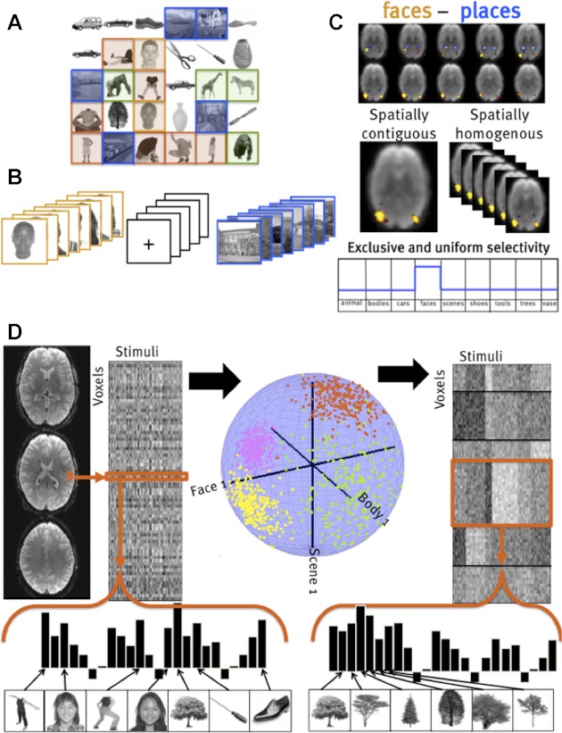
Comparison of classical contrast methods and the functional clustering approach. A–C: in a traditional contrast-based method, images are grouped into categories (A; faces, scenes, animals). Images from one presumed category are presented in blocks (B). Regression coefficients for blocks of images from 1 category are subtracted from another to form contrast maps (C); the resulting regions are evaluated for validity by their anatomical contiguity, anatomical homogeneity across subjects, and exclusive selectivity to the positive contrast. D: instead, functional clustering considers the response of each voxel to each image, the voxel's “response profile.” These response profiles are then normalized, and canonical “system profiles” are found that best account for the variation of responses across voxels and stimuli, thus yielding groups of voxels (or “systems”) that share a common response profile across stimuli. The result is a parcellation of voxels into similar functional systems, as well as the canonical profiles of those systems.

The potential of the functional clustering approach used here can be best understood by contrasting it with other approaches to functional magnetic resonance imaging (fMRI) data analysis. Like whole brain analyses (Friston et al. 1995), functional clustering considers all of the voxels within some volume without presupposing which voxels may be relevant to a given function. However, like region-of-interest (ROI) approaches (Saxe et al. 2006), functional clustering groups voxels into functional systems and characterizes the response profiles of the functional systems it finds (Stiers et al. 2006). Importantly, unlike ROI methods (or cluster-corrected whole brain analyses), our method considers only the responses of voxels across conditions, ignoring their locations; thus, like time-course clustering methods (Bartels and Zeki 2004; Golland et al. 2007), the functional clustering approach does not require anatomical proximity of functionally similar voxels (Simon et al. 2004; Thirion et al. 2006). This feature enables us to test, rather than assume, whether functionally similar voxels cluster together in the ventral visual pathway and arise in similar locations across subjects. Unlike independent component analysis applied to fMRI data (Beckmann and Smith 2004; Himberg et al. 2004; McKeown et al. 1998), our functional clustering method aims to partition voxels into functionally similar groups, rather than to describe the response of each voxel as an additive mixture of a number of functional responses. Like stimulus clustering methods (Kriegeskorte et al. 2008b), functional clustering does not presuppose which images group together or which functional profiles might best characterize brain responses (Mitchell et al. 2008), but instead discovers that grouping by finding sets of voxels with similar profiles of response across stimuli. However, by explicitly grouping voxels rather than stimuli, functional clustering aims to characterize partitions of neural functions rather than partitions of tasks or stimuli. Unlike voxel tuning function approaches (Serences et al. 2009), which seek to find receptive fields for individual voxels that collectively provide the basis for image representation (Kay et al. 2008), our method finds a small number of response profiles that characterize a large number of voxels. Thus functional clustering offers a novel approach to unsupervised analysis of large groups of voxels without presuming their anatomical distribution or functional properties and discovers which response profiles are most robust (i.e., present in many voxels, consistently across subjects), including novel response profiles not hypothesized in advance.

Previously, we tested this approach with eight stimulus categories in a blocked-design experiment and found that face, place, and body selectivity were among the top five most consistent profiles in the ventral steam (Lashkari et al. 2010). Moreover, when categories were split into different sets of images, functional clustering produced the same face-, place-, and body-selective response profiles, implicitly discovering that the two sets of images were from the same category (Fig. 2). Although this test relaxed many unwarranted assumptions of prior work, it only considered eight categories hypothesized in advance.

Fig. 2.

Blocked functional clustering data from 11 subjects: the top five systems most consistent across subjects include systems selective for bodies, faces, and scenes. Each bar represents different blocks with different stimulus sets. Inset pie charts represent the proportion of ventral stream voxels included in this system, and the histograms at right show the across-subject consistency score (blue) compared with the null-hypothesis distribution obtained via permutation tests. Selective systems that are consistent across subject, stimulus sets, and data sets show clearly that body (system 2), face (system 3), and scene selectivity (system 4) are evident.

In the present study, we attempted to discover the special categories in the brain by considering unique images without assuming how they group into categories. We scanned subjects viewing 69 images in an event-related design and applied functional clustering to response profiles over images (not categories), thus finding the stable profiles out of a space of about 10¹⁹ possibilities.² Face, place, and body selectivity represent a tiny fraction of the possible response profiles; are they still dominant when tested against the large space of possible response profiles tested here, and are there other, previously unknown, robust response profiles in the ventral visual pathway?

MATERIALS AND METHODS

Functional MRI data acquisition and analysis.

This research was approved by the MIT Institutional Review Board. Eleven subjects were scanned in an event-related design (6 female). Each subject was scanned in two 2-h scanning sessions (functional data from the 2 sessions were coregistered to the subject's native anatomical space). During the scanning session, the subjects saw rapid event-related presentations of 69 unique images drawn from 9 categories (animals, bodies, cars, faces, scenes, shoes, tools, trees, vases; Fig. 3). Images were presented in a pseudorandomized design generated by optseq (Dale 1999) to optimize the efficiency of regression of individual images, with no information about which images belong to which categories. During each 1.5-s presentation, the image moved slightly across the field of view either leftward or rightward, and subjects had to identify the direction of motion with a button press. The images subtended about 10 degrees of visual angle at fixation; subjects were asked to fixate, but their eye movements were not monitored. Half of the images were presented in session 1, and the other half were presented in session 2.

Fig. 3.

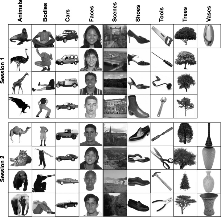
All 69 images used in the experiment are shown, grouped by category and session in which they appeared.

Functional MRI data were collected on a 3T Siemens scanner using a Siemens 32-channel head coil. The high-resolution slices were positioned to cover the entire temporal lobe and part of the occipital lobe (gradient echo pulse sequence, TR = 2 s, TE = 30 ms, 40 slices with a 32-channel head coil, slice thickness = 2 mm, in-plane voxel dimensions = 1.6 × 1.6 mm). Data analysis was performed with FreeSurfer Functional Analysis Stream (FS-FAST; http://surfer.nmr.mgh.harvard.edu), fROI (http://froi.sourceforge.net), and custom MATLAB scripts. The data were first motion-corrected separately for the two sessions (Cox and Jesmanowicz 1999) and then spatially smoothed with a Gaussian kernel of 3-mm width to increase the time-course signal-to-noise ratio (Triantafyllou et al. 2006).³ The clustering analysis was run on voxels selected for each subject for responding significantly to any one stimulus (omnibus F-test); we refer to the voxels selected in this manner as the search volume, or mask. We used standard linear regression to estimate the response of voxels to each of the 69 conditions, using a gamma hemodynamic response function with parameters δ = 2.25 and τ = 1.25 (Dale and Buckner 1997). We then registered the data from the two sessions to the subject's native anatomical space (Greve and Fischl 2009).

Functional clustering algorithm.

For a detailed mathematical treatment of the functional clustering algorithm, see appendix a and Lashkari et al. (2010). Below we provide a more intuitive overview of this method.

The functional clustering algorithm finds the set of voxel systems that best describe the response of all the voxels in a given search volume. To achieve this, functional clustering groups voxels by their selectivity profile, that is, their response pattern across a number of stimuli or tasks. Thus this method clusters voxels in the space of selectivity profiles; we call the resulting functional clusters “systems” to avoid confusion with the more common use of “cluster” in fMRI analysis to refer to spatial clusters of voxels. The resulting systems are characterized by their canonical selectivity profile, the average profile of all voxels in that system; thus all the voxels in that system may be concisely described as reflecting a particular functional response.

Functional clustering begins with the output of a conventional general linear model analysis, in which the response of a given voxel during the scan is modeled as a linear combination of responses to each stimulus/trial; the functional profile of a given voxel is then characterized as the maximum likelihood beta weights (regression coefficients) for each stimulus regressor. Thus, in our experiment with 69 different stimuli, the functional response of each voxel is characterized by a 69-unit vector of regression coefficients (1 for each of the 69 stimuli).

These regression coefficients reflect a number of functional and physiological properties of the voxel, including the selectivity of the voxel (its differential response across stimuli) and extraneous factors (such as proximity to the head coil and proximity to large blood vessels, which amplify signals both additively and multiplicatively). Because functional clustering aims to group voxels on the basis of their differential selectivity to stimuli, rather than their overall signal strength or proximity to blood vessels, we normalize the regression coefficient vectors to unit magnitude. Thus the functional profile of a voxel becomes a unit vector that reflects the relative response of that voxel to each of the presented stimuli, independently of the voxel's overall magnitude of response.

After normalization, the functional response of each voxel can be described as a point on a 68-dimensional hypersphere (see Fig. 1). Functional clustering then finds the set of K clusters that most effectively summarize the distribution of all voxels on this hypersphere such that each voxel is assigned to one cluster. Our model describes the distribution of selectivities across voxels as a mixture of von Mises-Fisher distributions (an analog of Gaussian distributions on the hypersphere). Thus we find the K hypersphere clusters that best describe the distribution of voxel functional profiles (see also Lashkari, 2010).

Functional clustering thus yields a parcellation of all voxels into K systems defined by their stimulus preference and corresponding response profiles that describe the canonical stimulus preference for each system. Crucially, this clustering is blind to the spatial distribution of voxels and finds functional systems defined only by the stimulus preference of voxels, regardless of their anatomical distribution.

Evaluating consistency across subjects and hypothesis testing.

Regardless of the underlying structure of the data, functional clustering will identify K systems; evaluating whether those systems are meaningful is a difficult statistical problem. We consider a system meaningful if it is robust across stimuli, if it replicates across within-subject data sets, and most importantly, if it is consistent across subjects. Because there is no known statistical test that assesses the consistency of clustering results, we adopt a method that computes an across-subject consistency score and tests these consistency scores against a rigorous null hypothesis computed via resampling.

To obtain a consistency score across subjects, we run our clustering algorithm 1) on all the voxels from all subjects, thus obtaining a clustering for the group, and then 2) on each subject independently, thus obtaining a separate clustering for each subject. We then match the individual subject systems to the closest group system to maximize the average correlation between the functional profiles of paired systems [using a standard combinatorial optimization procedure known as the Hungarian algorithm (Kuhn 1955)]. We do this for each subject and then obtain an average across-subject consistency score for a given system as the average over all correlations between the profile of the group system and those of matched individual subject systems.

Because this procedure identifies the best possible correspondence between individual subject systems and the group system, the expected value of the consistency score for a given system, even if there is no consistent structure in the data, will be greater than zero. Thus we can only ascertain the significance of our consistency scores by building an appropriate null-hypothesis distribution via permutation tests.

To run a permutation test, we must randomly shuffle our data to get rid of some structure that we think is present but that would not be present under the null hypothesis. We then rerun our analysis to obtain consistency scores without this structure. By repeating this procedure many times, we can build a null-hypothesis distribution appropriate for our across-subject consistency scores, and we will be able to ascertain the significance of our consistency scores compared with the appropriate null hypothesis. However, we must first decide what to shuffle to get rid of the structure that should not be present under the null hypothesis.

The conventional null hypothesis in most statistical tests in neuroscience is the assumption of a complete lack of structure; in other words, there is no stable mapping between stimuli and voxel responses in any subject in any voxel. To achieve this null hypothesis, we can randomly shuffle the mapping of images onto regressors. Thus, for each random permutation, each regressor will reflect a random set of stimulus events drawn from all images, so all regressors are drawn from the same distribution and have no structure. This would produce the expected distribution of consistency scores if our data contain no structure and our regressors are completely meaningless within each subject.

We adopt a more conservative null hypothesis by assuming that there is structure within subjects but no structure across subjects. In other words, the responses of voxels to different stimuli are systematic in each subject, but this mapping is not consistent across subjects. To do this, we construct the regressors within each subject as we do in the full analysis, so that each regressor within a subject corresponds to a specific image, but we permute the regressors across subjects. Thus the regressor corresponding to the presentations of the first face stimulus would be labeled “1” in one subject and might be labeled “5” in another subject (for whom the first regressor may correspond to the third scene). Using this across (but not within)-subject shuffling, we maintain the structure within subjects but eliminate the structure across subjects, thus giving us a more conservative test of across-subject system consistency than within-subject shuffling. For each such permutation, we compute the consistency scores for all 10 systems and include those in our null-hypothesis distribution. This null-hypothesis distribution over consistency scores, along with the actual observed consistency scores on the real data, is displayed in Fig. 5.

Fig. 5.

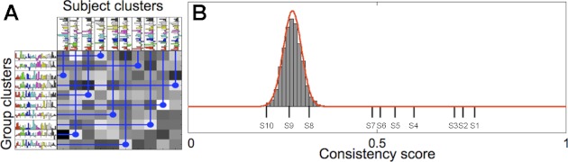
A: to obtain consistency scores, group clusters were matched to individual subject clusters. To test whether the resulting consistency scores were greater than expected by chance, we carried out randomization tests (see materials and methods) to construct a null-hypothesis distribution for consistency scores. B: histogram shows the empirical null-hypothesis distribution, the best-fitting beta distribution (red line), and the observed consistency scores for the 10 systems (S1–S10) shown in Fig. 4.

Assessing the selectivity of a functionally defined system in event-related data.

To quantify how well a profile matches a category, we first identify a candidate category on the basis of which image elicited the largest response. For instance, if the image eliciting the greatest response was a face, we would suppose that the cluster might be face selective. We then evaluate how well the cluster picks out the face category by using its response to all the other images (excluding the image with the highest response, which was used to select the hypothesis). To determine how well a profile picks out a particular image category, we construct a receiver operating characteristic (ROC) curve, where we start with the second highest response and assess whether it is a member of the target category (hit) or not (false alarm); we proceed to the next highest image, and so forth. Thus we can construct an ROC curve that represents the proportion of hits as a function of the proportion of false alarms, and we can assess the sensitivity, or selectivity, of the functional profile to a given category by the area under the curve of this ROC plot. We compute significance tests on this value via permutation tests of images and their associated ranks.

RESULTS

First, we estimated the response magnitude of each voxel in the ventral pathway to each of the 69 distinct images (see Fig. 3) in each of 11 subjects. We then applied our functional clustering algorithm to this data set, in effect searching for the 10 most prominent response profiles over the 69 images in the ventral visual pathway. Figure 4 shows the results of this analysis with each of the 10 response profiles (here called “systems”; see appendix b for stability of our key results with different numbers of clusters). We assessed whether the detected systems were significant (more reliable across subjects than would be expected by chance) under the null hypothesis that assumes no shared structure across subjects (see Fig. 5 and materials and methods); this analysis showed that systems 1–7 are significant at P < 0.001 each, but systems 8–10 are not significant (P > 0.5 each). The significant systems include profiles that appear upon visual inspection (see Figs. 4 and 6) to be selective for bodies (system 1), faces (system 2), and places (scenes; system 3).

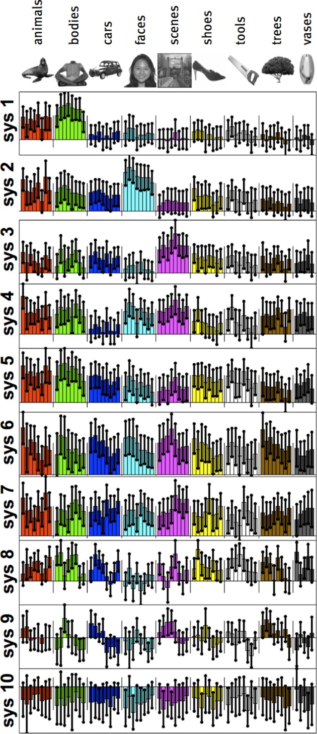
Fig. 4.

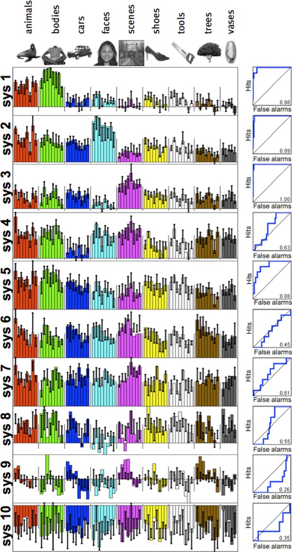
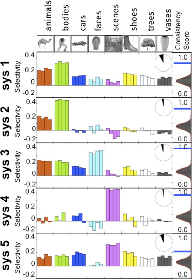
System profiles defined over 69 unique images. Each plot corresponds to 1 identified system (of 10 in total). Systems are plotted with consistency scores decreasing from top to bottom. Colored bars represent the response profile magnitude for the group cluster, whereas error bars represent the 75% interquartile range of the matching individual subject clusters (see materials and methods). Receiver operating characteristic (ROC) curves at right show how well the system profile picks out the preferred image category (defined by the image with the highest response), as evaluated on the other 68 images. As described in text, systems 1–7 are significantly consistent across subjects, whereas systems 8–10 are not.

Fig. 6.

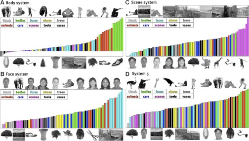
Stimulus preference for the apparently selective systems: body (A; system 1), face (B; system 2), scene (C; system 3), and unidentified (D; system 5). For each system, the set of images above the rank-ordered stimulus preference shows the 10 most preferred stimuli, and the images below show the 10 least preferred stimuli.

To confirm the intuition that these profiles are in fact selective for faces, bodies, and scenes, we computed ROC curves for how well each response profile picks out a preferred category. For each cluster we tested selectivity for the category of the image to which that cluster was most responsive (thus, if the cluster was most responsive to a face, we propose that it is “face selective”), and then we used the other 68 images to compute an ROC curve describing how precisely this profile selects the identified image category (see materials and methods). Figure 2 shows the ROC curves for the 10 identified clusters; via permutation tests, we found that the areas under the curve for the face, body, and scene systems are all statistically significant (all P < 0.001); system 5 (selective for either bodies or animals) is also highly significant (P < 0.001), but all other systems show no significant category selectivity (all P > 0.1). At the same time as these systems have reliable category selectivity, the specific rank ordering of preferred images within the body (Fig. 6A), face (Fig. 6B), and scene systems (Fig. 6C) shows substantial variation in the magnitude of response to different exemplars from these categories. Although these systems are well characterized by selectivity for the a priori categories, they do not respond homogenously to all stimuli within each category, and there is some variability across voxels within a given system (see appendix c).

To quantitatively assess the robustness and reliability of identified clusters, we tested whether the selectivity is reliable when evaluated with respect to independent images that were not used for clustering. Thus we split our image set into two halves, with four images from each category in each half of the data. We then used one half of the image set for functional clustering and the other half to assess the stability of the selectivity of the identified functional systems. Specifically, we analyzed the response magnitude to the second half of the stimuli in voxels that were clustered into a given system using the first half of the stimuli. Figure 7 confirms the across-image reliability of category selectivity for the first four systems: selectivity identified by functional clustering in one half of the images is replicated in the second half of the images.

Fig. 7.

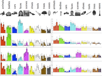
Consistency of clustering results across independent images. Half of the images were used for functional clustering, the voxels corresponding to these clusters were selected as functional regions of interest (ROIs), and the responses of these regions were assessed in the other, independent half of the images. Data at left are the clustering results (displayed as in Fig. 4), whereas data at right are the matching average response magnitudes in the other half of the images in each system's voxels.

The analyses described so far demonstrate that from the large space of possible response profiles that could be discovered in our analysis, response profiles reflecting selectivity for faces, bodies, and places emerge at the top of the stack, indicating that they are some of the most dominant response profiles in the ventral pathway.

New selectivities?

Next, we turn to the question of whether our analysis discovers any new functional systems not known previously. Beyond the systems that clearly reflect selectivity for faces, places, and bodies, there are four other significant systems (systems 4–7 in Fig. 4). A comparison of these profiles with those of systems derived from occipital regions of cortex (see Fig. 8) shows that three of these systems resemble one or more of the selectivity profiles derived from occipital cortex: system 4 from the ventral cortex resembles system 1 from occipital cortex, ventral system 6 resembles occipital system 4, and ventral system 7 resembles occipital system 7 (r > 0.8 in all cases), suggesting that these response profiles reflect the kind of basic visual properties extracted in occipital cortex.

Fig. 8.

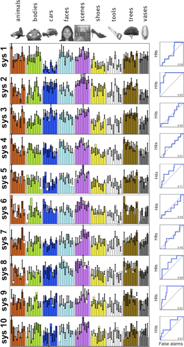
Clustering results on occipital areas. The dominant selective profiles found in the ventral stream do not appear when clustering results of systems derived from occipital cortex, suggesting that they reflect higher order structure rather than low-level image properties. As in Fig. 4, bars represent the response profile magnitude for the group cluster, whereas error bars represent the 75% interquartile range of the matching individual subject clusters (see materials and methods).

Thus the significant systems discovered by our algorithm include the three known category selectivities (systems 1–3) plus three systems that appear to reflect low-level visual properties (or at least resemble the selectivities that emerge from occipital cortex). The one remaining significant system, which does not strongly resemble any occipital profile, is system 5. Visual inspection of the stimuli that produce particularly high and low responses in this system (see Fig. 6D) does not lead to obvious interpretations of the function of this system. (It is tempting to label this system as selective for “animate objects” or “living things” because of the high responses to bodies and animals, but neither classification can explain the low response of this system to faces and trees.) This situation reveals both the strength of our data-driven functional structure discovery method (its ability to discover novel, unpredicted response profiles) and its weakness (what are we to say about these response profiles once we find them?). A full understanding of the robustness and functional significance of system 5 will have to await further investigation.

Projecting voxels of each system on their anatomical locations.

Crucially, all of the analyses described so far were blind to the anatomical location of each voxel. Thus the functional clustering procedure makes no explicit assumptions about the spatial contiguity of voxels within a system,⁴ nor does it presume that voxels within each system will be in anatomically similar locations across subjects. This analysis thus enables us to ask two questions that are implicitly assumed in standard group analyses (as well as cluster size-corrected and ROI-based analyses): 1) Do voxels with similar response profiles tend to be near each other in the brain? and 2) Do voxels with similar response profiles indeed land in similar anatomical locations across subjects? The answer to both questions is yes, as revealed by inspection of maps of the anatomical location of the voxels in each significant system in each subject (see Fig. 9 and appendix d for across-subject system size variability). The anatomical locations of the voxels in systems 1, 2, and 3 clearly match the well-established cortical regions selective for bodies, faces, and scenes (Kanwisher, 2010), showing both spatial clustering within each subject for each system and similarity in anatomical location across subjects.

Fig. 9.

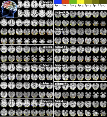
Significant systems projected back into the brain of subject 1. As can be seen, systems 4, 6, and 7 arise in posterior, largely occipital regions around the calcarine sulcus. Category-selective systems 1, 2, and 3 arise in their expected locations. System 5 appears to be a functionally and anatomically intermediate region between retinotopic and category-selective cortex.

The spatial clustering apparent upon visual inspection of Fig. 9 can be quantified by analyzing the probability of spatial co-occurrence at different scales (see appendix e). For each voxel of each system, within each subject, we calculate the proportion of voxels a given distance away that are members of the same system. We also compute this quantity for randomly selected voxels from within the search volume to correct for the base rate of voxels within any given system. In Fig. 10, we plot the logarithm of the ratio of these real and random co-occurrences. As shown, for all systems these log ratios at short distances are greater than zero, indicating that all systems are more spatially clustered than would be expected from random dispersion throughout the search volume. However, importantly, the face-, scene-, and body-selective systems are more spatially clustered than system 5 or the apparently nonselective systems, indicating that these category-selective regions tend to cluster spatially more than nonselective systems.

Fig. 10.

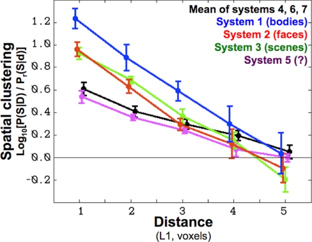
Degree of spatial clustering (y-axis) for each system plotted as a function of distance (x-axis). This measure corresponds to the likelihood that voxels from the same system tend to be close together, more so than would be expected by random dispersion throughout the search volume (see appendix e). Because the y-axis is in log base-10 units, a value of 1 indicates that voxels from a given system are 10 times more likely to cluster at this distance from other voxels of this system than randomly selected voxels from within the mask. All systems show some degree of spatial clustering (clustering >0), which should be expected given the smoothness of fMRI data; however, the selective systems show 2 to 4 times as much spatial clustering as nonselective systems.

Furthermore, when the voxels in systems 4, 6, and 7 (shown above to resemble profiles that emerge from occipital cortex) are projected back into the brain, they indeed appear mainly in posterior occipital regions known to be retinotopic (see Fig. 9), confirming our previous analysis that they reflect early stages of visual processing and do not reflect noteworthy high-level selectivity.

Finally, further evidence that the new functional profile, system 5, is indeed a novel selectivity worthy of further investigation comes from the fact that it, too, contains a largely contiguous cluster of voxels that is anatomically consistent across subjects. Specifically, the spatial map of system 5 consistently includes areas on the lateral surface of both hemispheres that begin inferiorly near and are sometimes interdigitated within, but largely lateral to, face-selective voxels, extending up the lateral surface of the brain to more superior body-selective regions.

DISCUSSION

In this experiment, we searched the large space of all possible response profiles over 69 stimuli with no assumptions about 1) which of these stimuli go together to form a category, 2) what kind of response profile is expected (from an exclusive response to a single stimulus, to a broad response to many), or 2) whether voxels with similar response profiles occur in similar locations across subjects. Despite relaxing these assumptions, present in almost all prior work on the ventral visual pathway, we nonetheless found that three of the four most robust response profiles represent selectivity for faces, places, and bodies. Although in some sense this finding is a rediscovery of what we already knew, it is a very powerful rediscovery, because it shows that even when the entire hypothesis space is tested, with all possible response profiles on equal footing, these three selectivities nonetheless emerge as the most robust. Put another way, this discovery suggests that the observed dominance of these response profiles in the ventral visual pathway has not been due to the biases present in the way the hypothesis space has been sampled in the past but to inherent properties of the ventral visual pathway.

In addition to finding face, place, and body selectivity, our clustering algorithm found four other significant systems. Three of these reflect low-level visual analyses conducted in occipital cortex, as evidenced both by the similarity of their response profiles to the profiles arising from occipital cortex and by the anatomical location where these voxels are found, in posterior occipital cortex. Can our analysis discover any new response profiles not predicted by prior work? Indeed, one significant system (system 5) revealed a new selectivity profile that was not predicted and that does not strongly resemble any of the profiles originating in occipital cortex. But the unique ability of our method to discover novel, unpredicted response profiles also raises the biggest challenge for future research: What can we say about any new response profiles we discover, if (as for system 5) they do not lend themselves to any straightforward functional hypothesis? Of course, the first question is whether such novel profiles will replicate in future work. If they do, their functional significance can be investigated by probing with new stimuli to test the generality and specificity of the response of these systems.

A further result of our work is to show that category selectivities in the ventral pathway cluster spatially at the grain of multiple voxels. Although this result is familiar from many prior studies, the methods used in those studies generally built in assumptions of spatial clustering either explicitly (e.g., with cluster size thresholds or ROI-based analyses) or implicitly (because discontiguous and scattered activations are usually discounted as noise). In contrast, our analysis was conducted without any information about the location of the voxels (see also Fig. 10), yet the resulting functional systems it discovered, when projected back into the brain, are clustered in spatially contiguous regions more often than expected by chance or than nonselective systems (see Figs. 9 and 10). Because the spatial clustering of these regions was not explicitly assumed in our analysis, the fact that those voxels are indeed spatially clustered reflects a new result.

Important caveats remain. First, although our method avoids many of the assumptions underlying conventional contrast-driven fMRI analysis, we cannot eliminate the basic experimental choice of stimuli to be tested. The set of stimuli in our experiment was designed to include images drawn from potentially novel categories as well as previously hypothesized categories, which allowed us to simultaneously validate the method on previously characterized functionally selective regions and to potentially discover new selectivity profiles. Moreover, although we included images of some plausible categories, we sampled each category equally, rather than over-representing images from any one category (such as faces or animals). Nonetheless, for a completely unbiased approach, one would need to present images that were chosen independently of prior hypotheses (e.g., a representative sampling of ecologically relevant stimuli). A related caveat concerning the present results is that we do not know what other functionally defined systems may exist whose diagnostic responses concern stimuli not sampled in our experiment, and whether those systems may prove more robust than those discovered in the present analysis. In ongoing work we are addressing these concerns by applying our methods to data obtained from a larger number of stimuli, sampled in a hypothesis-neutral fashion.

A second caveat is that our analysis searches for functional profiles that each characterize a large number of voxels; therefore, we cannot rule out the possibility that many voxels in the ventral stream may contain idiosyncratic functional profiles, each characterizing only a small number of voxels. Thus the fact that our analysis discovers category selectivities as the most robust profiles does not preclude the possibility that the ventral pathway also contains a large number of other voxels, each with a unique, but perhaps less selective, profile of response over a large number of images. Such additional voxels could collectively form a distributed code for object identity or shape, represented as a particular pattern of responses over a large set of voxels, each with a slightly different profile of response (Haxby et al. 2001). The image categories implied by such distributed codes can be assessed by methods that cluster images by the similarity of the neural response they evoke (as opposed to our approach of clustering voxels by the similarity of their responses across images) (Drucker and Aguirre 2009; Haushofer et al. 2008; Kriegeskorte et al. 2008a). These stimulus-clustering approaches have yielded stimulus categories roughly consistent with the category-selective systems we find: a distinction between animate and inanimate images, and a further distinction between faces and bodies (Kriegeskorte et al. 2008b), suggesting that the image categories defined over the whole ventral visual stream are dominated by the few category-selective areas we report in this article.

Our method also cannot circumvent the difficulty of characterizing a functional response. For instance, consider the face-, place-, and body-selective systems that we find; what aspects of the stimuli yield such a grouping? These different stimulus categories have different image-level correlates, both at a coarse level (faces tend to be round, scenes were rectangular images) and at more subtle levels (scenes tend to contain higher spatial frequencies and larger fields of view). appendix f shows that our image set contains coarse category-level image correlations; however, even if these first-order correlations are removed, other image-level correlations will necessarily remain. Thus the current method cannot determine whether the response profiles we find reflect abstract semantic categories or complex image statistics: answering these questions requires focused experiments aimed to test specific hypotheses about which image-level properties produce selectivity for specific image categories, such as those that have been carried out for the past decade on the face- and place-selective regions (Kanwisher 2010; Walther et al. 2011; Wolbers et al. 2011; Yue et al. 2011). Thus any systems discovered by functional clustering will still need to undergo thorough and rigorous testing to characterize their precise nature.

Despite these caveats, the current study has made important progress. Specifically, we found that even when the standard assumptions built into most imaging studies (spatial contiguity and spatial similarity across subjects of voxels with similar functional profiles) are relaxed or eliminated, and even when we give an equal shot to the vast number of all possible functional response profiles over the stimuli tested, we still find that selectivities for faces, places, and bodies emerge as the most robust profiles in the ventral visual pathway. Our discovery indicates that the prominence of these categories in the neuroimaging literature does not simply reflect biases in the hypotheses neuroscientists have thought to test, but rather that these categories are indeed special in the brain. Future research must include even more stringent tests of the dominance of these category selectivities by testing each subject on a larger number of stimuli selected in a completely hypothesis-neutral fashion. This approach enables us to discover new response profiles in the ventral visual pathway that were not previously known from more conventional methods and also opens up an avenue for rich, unsupervised analyses of data from fMRI repositories.

GRANTS

This work was funded by National Institutes of Health (NIH) National Eye Institute Grant EY-13455 to N. Kanwisher and National Science Foundation (NSF) Information & Intelligent Systems/Collaborative Research in Computational Neuroscience Grant 0904625, NSF CAREER Award 0642971, NIH National Institute of Biomedical Imaging and Bioengineering (NIBIB) Neuroimaging Analysis Center Grant P41-EB-015902, and NIH NIBIB National Alliance for Medical Image Analysis Grant U54-EB005149 to P. Golland.

DISCLOSURES

No conflicts of interest, financial or otherwise, are declared by the authors.

AUTHOR CONTRIBUTIONS

E.V., D.L., P.G., and N.K. conception and design of research; E.V. and P.-J.H. performed experiments; E.V. and D.L. analyzed data; E.V., D.L., P.-J.H., P.G., and N.K. interpreted results of experiments; E.V., D.L., and P.-J.H. prepared figures; E.V. and N.K. drafted manuscript; E.V., D.L., P.-J.H., P.G., and N.K. edited and revised manuscript; E.V., P.G., and N.K. approved final version of manuscript.

APPENDIX A: TECHNICAL DETAILS OF THE FUNCTIONAL CLUSTERING APPROACH

Here we formally describe the probabilistic model underlying our functional clustering analysis; a more detailed technical description and derivation of the algorithms used for clustering may be found in Lashkari et al. (2010).

Functional clustering operates over the selectivity profiles of each of V voxels. The selectivity profile of voxel i (s_i) is the vector of all 69 regression coefficients (B) corresponding to that voxel's response to each stimulus, normalized to unit length:

$$s_i=\frac{\overrightarrow{B}}{\Vert \overrightarrow{B}\Vert },$$

where ‖B‖ is the vector norm.

These unit-length vectors, which we call “selectivity profiles,” are a projection of the 69 regression coefficients onto a 68-dimensional sphere.

Our clustering model assumes that all of the selectivity profiles (the s_i unit vectors) are independently and identically distributed according to a mixture of K clusters. Each cluster (k) is described by a circular Gaussian distribution (a von Mises-Fisher distribution) on the 68-dimensional sphere. The cluster is parameterized by a particular mean (m_k), the canonical profile of all voxels within that cluster, and a concentration parameter (λ), the spread of selectivity profiles around the mean. We use one concentration parameter for all clusters.

The probability of an individual observation is given by the mixture model:

$$P\left(s_i|{\left\{q_k,m_k\right\}}_{k=1}^K,\lambda \right)={\displaystyle \sum _{k=1}^K{q}_{k}P\left(s_i|m_k,\lambda \right),}$$

where q_k is the weight assigned to a given cluster (roughly, the frequency with which voxels tend to belong to that cluster). The probability of a given selectivity profile under a given cluster is given by the von Mises-Fisher distribution:

$$P\left(s_i|m_k,\lambda \right)=Z_D\left(\lambda \right)\exp \left[\lambda \langle s_i,\hspace{0.17em}{m}_k\rangle \right],$$

where <x,y> is the dot product of x and y (for unit vectors, this is the correlation), so in our case, it is the correlation of the voxel selectivity profile with the canonical cluster profile. Z_D is the normalizing constant for the von Mises-Fisher distribution, defined in terms of the modified Bessel function of the first kind and order D/2−1 (I_D/2−1), where D is the dimensionality of the sphere.

$$Z_D\left(\lambda \right)=\frac{{\lambda }^{D/2-1}}{{\left(2\pi \right)}^{D/2}{I}_{D/2-1}\left(\lambda \right)}$$

We obtain the maximum likelihood parameters (the concentration parameter λ, the q_k cluster weights, and the m_k cluster centers) by optimization:

$$\begin{array}{c}\arg \max \\ {\left\{q_k,\hspace{0.17em}{m}_k\right\}}_{k=1}^K,\lambda \end{array}={\displaystyle \sum _{i=1}^V\log P\left(s_i|{\left\{q_k,\hspace{0.17em}{m}_k\right\}}_{k=1}^K,\lambda \right)}$$

We solve this optimization problem via an expectation-maximization algorithm, where we iteratively compute the probability that each voxel i is assigned to each cluster k (the expectation step):

$$p_i\left(k|s_i\right)=\frac{q_i\hspace{0.17em}\exp \left[\lambda \langle s_i,m_k\rangle \right]}{{\displaystyle {\sum }_{k\prime =1}^K{q}_{k\prime }\hspace{0.17em}\exp \left[\lambda \langle s_i,m_{k\prime }\rangle \right]}}.$$

Using these assignment probabilities, in the maximization step we update the cluster weights,

$$q_k=\frac{1}{V}{\displaystyle \sum _{i=1}^V{p}_i\left(k|s_i\right);}$$

the cluster centers,

$$q_k=\frac{{\displaystyle \sum _{i=1}^V{s}_i{p}_i\left(k|s_i\right)}}{\Vert {\displaystyle \sum _{i=1}^V{s}_i{p}_i\left(k|s_i\right)}\Vert };$$

and the concentration parameter. Updating the concentration parameter amounts to solving the following nonlinear equation:

$$\frac{I_{D/2}\left(\lambda \right)}{I_{D/2-1}\left(\lambda \right)}=\frac{1}{V}{\displaystyle \sum _{k=1}^K{\displaystyle \sum _{i=1}^{K}p\left(k|s_i\right)\langle m_k,\hspace{0.17em}{s}_i\rangle },}$$

and we can approximate this solution as

$$\lambda \approx \frac{\left(D-1\right)\Gamma }{1-{\Gamma }^2}+\frac{D\Gamma }{2\left(D-1\right)},$$

where

$$\Gamma =\frac{1}{V}{\displaystyle \sum _{k=1}^K{\displaystyle \sum _{i=1}^{K}p\left(k|s_i\right)\langle m_k,\hspace{0.17em}{s}_i\rangle .}}$$

(See appendix a and appendix b of Lashkari et al. 2010 for a derivation of this approximation, as well as derivations of the specific update rules used in the expectation-maximization algorithm.)

APPENDIX B: RESULTS FOR DIFFERENT NUMBERS OF CLUSTERS

Clustering results for different numbers of clusters are shown in Fig. B1 (in left, middle, and right panels, k = 15, k = 20, and k = 25, respectively). As more clusters are included, some of the functionally selective systems we see in the main (k = 10) results are split into several groups; for instance, system 1 from k = 15 appears to match system 1 from k = 10, but in k = 25, this “animal/body” selective system appears as both system 2 and system 3, which differ slightly in the degree to which they respond to other stimuli. It seems that most of the other additional systems correspond to further splitting the large undifferentiated systems that respond nonselectively to the set of images we tested.

Fig. B1.

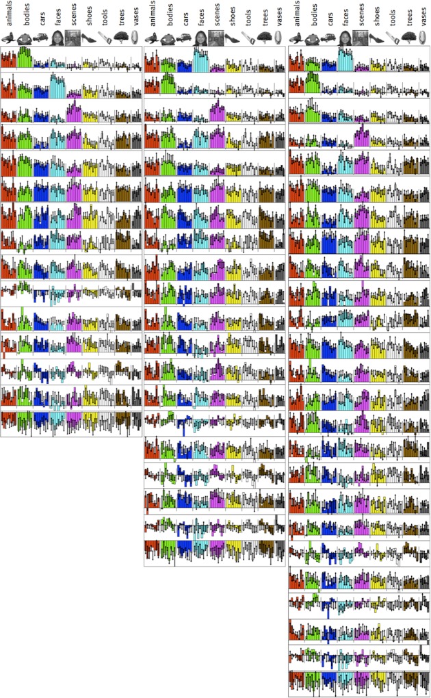
Clustering results for k = 15, 20, and 25.

APPENDIX C: VARIABILITY WITHIN AND ACROSS VOXELS OF A GIVEN SYSTEM

Figure C1 shows the mean system responses (as in Fig. 4), but the error bars here correspond to ±1 SD across voxels within the system. It should be noted that these graphs are only useful to assess how well the clustering algorithm achieved its task of grouping voxels with similar response profiles together.

Fig. C1.

Mean system responses (as in Fig. 4), but with error bars corresponding to ±1 SD across voxels within the system.

The measures reported in Fig. C1 correspond to the degree to which voxels grouped into a given system vary around the response profile and the degree to which those voxels are selective for a particular set of images. In principle, one can quantify the effect size corresponding to the profile by using η², the proportion of the total variability of voxel-stimulus responses in a given system that can be accounted for by the variability in average responses to a given image (this is an r² measure for qualitative factors). However, because voxels were grouped to form systems with similar response profiles, the variability across voxels within a system will be underestimated, and the effect size measure will be inflated. We report these inflated scores in the third column of Table C1 but note that even systems that are not significant across subjects show relatively high numbers.

Table C1.

Mean, SD, and range of number of voxels (and volume) included in each system from each subject

System	Mean No. of Voxels	SD No. of Voxels	Min.–Max No. of Voxels
1 (Animals/bodies)	189 (968)	114 (584)	1 (5)–346 (1,772)
2 (Faces)	302 (1,546)	131 (671)	122 (625)–604 (3,093)
3 (Scenes)	441 (2,258)	307 (1,572)	129 (661)–1,207 (6,180)
4*	353 (1,807)	151 (773)	119 (609)–601 (3,077)
5 (?)	842 (4,311)	428 (2,191)	239 (1,224)–1,653 (8,463)
6 (*)	1,026 (5,253)	940 (4,813)	131 (671)–2,815 (14,413)
7 (*)	1,329 (6,805)	1,138 (5,827)	114 (584)–3577 (18,314)
8 NS	228 (1,167)	740 (3,789)	0 (0)–2,461 (12,600)
9 NS	26 (133)	58 (297)	0 (0)–198 (1,014)
10 NS	160 (819)	165 (845)	1 (5)–510 (2,611)

Values are mean, SD, and range of no. of voxels (with volume in parentheses, in mm³) included in each system from each subject. Systems marked with an asterisk match systems found in occipital cortex, suggesting that they reflect basic image properties. System indicated with a question mark is a significant system that does not strongly resemble any occipital profile (see text for details). Systems labeled “NS” showed no significance.

Specifically, we calculate the following quantities, where s_i,j is the normalized magnitude of the selectivity profile of voxel i (within a given system) to stimulus j: the mean (across all voxels in a system) response to a given image,

$${\overline{x}}_j=\frac{1}{n}{\displaystyle \sum _{i=1}^n{s}_{i,j};}$$

the variance of mean image responses in a system,

$${\widehat{\sigma }}_{img}^2=\frac{1}{69}{\displaystyle \sum _{j=1}^{69}{\left({\overline{x}}_j-\frac{1}{69}{\displaystyle \sum _{j=1}^{69}{\overline{x}}_j}\right)}^2;}$$

the variance of voxel selectivity profiles around the mean system profile to a given image,

$${\widehat{\sigma }}_{vox}^2=\frac{1}{69n}{\displaystyle \sum _{i=1}^{69}{\displaystyle \sum _{j=1}^{69}{\left(s_{i,j}-{\overline{x}}_j\right)}^2;}}$$

the total variance of voxel responses in a given system,

$${\widehat{\sigma }}_{tot}^2=\frac{1}{69n}{\displaystyle \sum _{i=1}^{69}{\displaystyle \sum _{j=1}^{69}{\left(s_{i,j}-\frac{1}{69n}{\displaystyle \sum _{i=1}^{69}{\displaystyle \sum _{j=1}^{69}{s}_{i,j}}}\right)}^2};}$$

and the proportion of total variance in voxel responses in a given system accounted for by the variation across mean image responses,

$${\eta }^2=\frac{{\overline{\sigma }}_{img}^2}{{\overline{\sigma }}_{tot}^2}.$$

(Note that this is effectively a measure of how well the clustering algorithm has served its intended purpose, because it is designed to group voxels with similar response profiles together).

In Table C1, we compare the variability of voxel responses within a given system to the variability of the mean response across images. Because voxels were grouped into systems on the basis of sharing a common response profile, the variability across voxels will be underestimated by the grouping, and even systems that are not significant across subjects will appear to have little across-voxel variation.

APPENDIX D: VOXELS/VOLUME IN A GIVEN SYSTEM

How stable are the different systems (in terms of their size) across subjects? In Table D1, we assess the stability by considering the mean, standard deviation, and range of the number of voxels (and volume in mm³) for the 10 systems included in the main analysis. Although the reliable systems show up in all subjects, the variability in system size across subjects is considerable.

Table D1.

Comparison of the variability of voxel responses within a given system with the variability of the mean response across images

System	Across-Image Response Variance, σ̂img2 × 103	Within-Image Across-Voxel Variance, σ̂vox2 × 103	Total Within-System Response Variance, σ̂tot2 × 103	Proportion 0f Total Within-System Variance Explained by Across-Image Variance, η2
1	5.2	5.8	10.9	0.48
2	2.4	4.1	6.5	0.37
3	2.2	5.0	7.1	0.31
4	1.9	4.2	6.0	0.31
5	1.1	3.5	4.5	0.24
6	0.8	3.4	4.2	0.18
7	0.7	3.2	3.9	0.19
8	3.6	4.8	8.4	0.43
9	5.3	9.2	14.5	0.37
10	0.6	8.6	9.2	0.07

Data compare the variability of voxel responses within a given system with the variability of the mean response across images. Because voxels were grouped into systems based on sharing a common response profile, the variability across voxels will be underestimated by the grouping, and even systems that are not significant across subjects will appear to have little across-voxel variation.

APPENDIX E: QUANTIFYING SPATIAL CLUSTERING

To quantify spatial clustering, we modify Ripley's K function (Ripley 1977), which is a common spatial statistics tool used to measure spatial clustering and dispersion. Specifically, we ask whether a voxel at distance d from a voxel belonging to system s is more likely to be part of that system than would be expected by random dispersion. We compare these spatial clustering metrics between the body-, face-, and scene-selective areas with the other, significant, apparently nonselective systems. This comparison yields a statistical test that can assess whether the selective systems we find are more spatially clustered than the nonselective systems.

First, we calculate the proportion of voxels at each distance that belong to the same system. We use L1 (city block) distance measured in voxels; thus a distance of 1 around a particular voxel corresponds to a 3 × 3 × 3-voxel cube, excluding the center voxel; a distance of 2 corresponds to a 5 × 5 × 5 cube shell (excluding the inner 3̂3 cube).

For each system s, we find all N_d voxels that are at distance d away from any one of the voxels within that system (but are still within our mask, the search volume used for all analyses). We then calculate what proportion of those voxels are in the same system, thus obtaining P_s(s|d), the probability that a voxel distance d away from a voxel in system s will also be in system s.

We repeat the same procedure for randomly selected seed voxels to correct for the base rate of the system. Specifically, for each voxel in system s, we choose a random seed voxel from within our mask (the search volume) and repeat the same analysis to compute P_r(s|d), the base rate co-occurrence probability established by random permutation.

Finally, we compute the ratio P_s(s|d)/P_r(s|d), which is a measure of how much more likely than chance are voxels within a given system to cluster together at distance d. We take the base 10 logarithm of this ratio to make the scale linear: log₁₀[P_s(s|d)/P_r(s|d)], so a value of 0 indicates that voxels in this system cluster no more than chance.

Figure 10 shows the across-subject average of this measure as a function of distance for the three selective systems, system 5, as well as the average over the significant, nonselective systems. All systems cluster more than would be expected by random dispersion (values greater than 0); this is expected given the inherent smoothness of fMRI data. More importantly, the face-, body-, and scene-selective systems are all more clustered at small distances than either nonselective systems or system 5.

APPENDIX F: IMAGE-LEVEL CORRELATIONS

Astute readers will note that some image-level properties are correlated with semantic category membership: scenes tend to be rich, full-frame images; faces tend to be round; cars tend to be flat; etc. To what extent do the systems that we find reflect image-level properties, and to what extent do they reflect higher level, semantic categories? From our data, or from any one experiment alone, this would be difficult to judge: our stimulus set was not designed to control for these image features, and even when carefully controlled, fully characterizing the response properties of a functional system requires many specially tailored experiments [e.g., characterizing the PPA required a comparison of landmarks, landscapes, furnished rooms, outdoor scenes, empty rooms, and independent walls of empty rooms (Epstein and Kanwisher 1998), and even so, new candidate low-level explanations will always remain (Rajimehr et al. 2011)]. This point can be illustrated by looking at the pixel-level correlations between images in different categories (Fig. F1): cars (images 17–24) and faces (images 25–32) are more correlated with themselves than other image categories given the unique and uniform shapes of those objects.

Fig. F1.

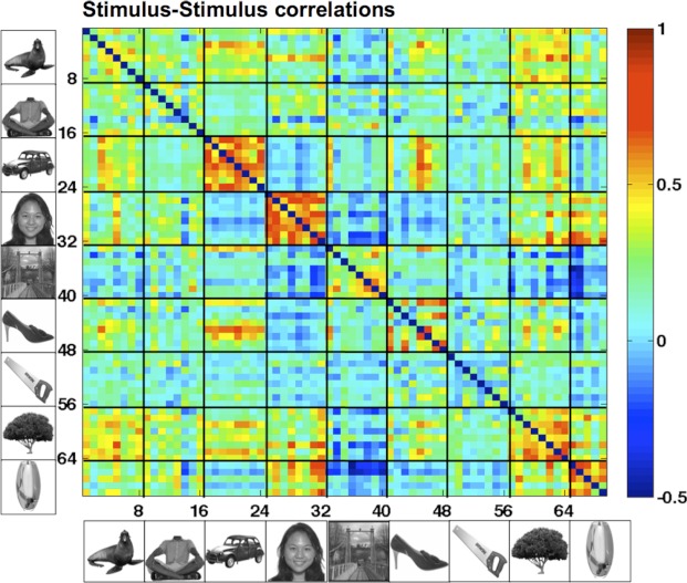
Stimulus-stimulus pixel-level correlations.

Nevertheless, our data do provide evidence that anatomically unconstrained functional clustering can identify the functional systems that others have reported in the past, showing that functional clustering is a promising tool for discovering new functional profiles. Any systems so discovered will subsequently need to be subjected to thorough testing to adequately characterize their function.

REFERENCES

- Baker CI, Liu J, Wald LL, Kwong KK, Benner T, Kanwisher N. Visual word processing and experiential origins of functional selectivity in human extrastriate cortex. Proc Natl Acad Sci USA 104: 9087–9092, 2007 [DOI] [PMC free article] [PubMed] [Google Scholar]
- Bartels A, Zeki S. The chronoarchitecture of the human brain—natural viewing conditions reveal a time-based anatomy of the brain. Neuroimage 22: 419–433, 2004 [DOI] [PubMed] [Google Scholar]
- Beckmann CF, Smith SM. Probabilistic independent component analysis for functional magnetic resonance imaging. IEEE Trans Med Imaging 23: 137–152, 2004 [DOI] [PubMed] [Google Scholar]
- Caramazza A, Shelton JR. Domain-specific knowledge systems in the brain the animate-inanimate distinction. J Cogn Neurosci 10: 1–34, 1998 [DOI] [PubMed] [Google Scholar]
- Chao LL, Martin A. Representation of manipulable man-made objects in the dorsal stream. Neuroimage 12: 478–484, 2000 [DOI] [PubMed] [Google Scholar]
- Chao LL, Haxby JV, Martin A. Attribute-based neural substrates in temporal cortex for perceiving and knowing about objects. Nat Neurosci 2: 913–919, 1999 [DOI] [PubMed] [Google Scholar]
- Cohen L, Dehaene S, Naccache L, Lehericy S, Dehaene-Lambertz G, Henaff MA, Michel F. The visual word form area: spatial and temporal characterization of an initial stage of reading in normal subjects and posterior split-brain patients. Brain 123: 291–307, 2000 [DOI] [PubMed] [Google Scholar]
- Cox RW, Jesmanowicz A. Real-time 3D image registration for functional MRI. Magn Reson Med 42: 1014–1018, 1999 [DOI] [PubMed] [Google Scholar]
- Dale AM. Optimal experimental design for event-related fMRI. Hum Brain Mapp 8: 109–114, 1999 [DOI] [PMC free article] [PubMed] [Google Scholar]
- Dale AM, Buckner RL. Selective averaging of rapidly presented individual trials using fMRI. Hum Brain Mapp 5: 329–340, 1997 [DOI] [PubMed] [Google Scholar]
- Downing PE, Jiang Y, Shuman M, Kanwisher N. A cortical area selective for visual processing of the human body. Science 293: 2470–2473, 2001 [DOI] [PubMed] [Google Scholar]
- Downing PE, Chan AW, Peelen MV, Dodds CM, Kanwisher N. Domain specificity in visual cortex. Cereb Cortex 16: 1453–1461, 2006 [DOI] [PubMed] [Google Scholar]
- Drucker DM, Aguirre GK. Different spatial scales of shape similarity representation in lateral, and ventral LOC. Cereb Cortex 19: 2269–2280, 2009 [DOI] [PMC free article] [PubMed] [Google Scholar]
- Epstein R, Kanwisher N. A cortical representation of the local visual environment. Nature 392: 598–601, 1998 [DOI] [PubMed] [Google Scholar]
- Friston K, Holmes A, Worsley K, Poline JP, Frith C, Frackowiak R. Statistical parametric maps in functional imaging: a general linear approach. Human Brain Mapp 2: 189–210, 1995 [Google Scholar]
- Golland P, Golland Y, Malach R. Detection of spatial activation patterns as unsupervised segmentation of fMRI data. Med Image Comput Comput Assist Interv 10: 110–118, 2007 [DOI] [PMC free article] [PubMed] [Google Scholar]
- Greve DN, Fischl B. Accurate and robust brain image alignment using boundary-based registration. Neuroimage 48: 63–72, 2009 [DOI] [PMC free article] [PubMed] [Google Scholar]
- Haushofer J, Livingstone MS, Kanwisher N. Multivariate patterns in object-selective cortex dissociate perceptual and physical shape similarity. PLoS Biol 6: e187, 2008 [DOI] [PMC free article] [PubMed] [Google Scholar]
- Haxby JV, Gobbini MI, Furey ML, Ishai A, Schouten JL, Pietrini P. Distributed and overlapping representations of faces and objects in ventral temporal cortex. Science 293: 2425–2430, 2001 [DOI] [PubMed] [Google Scholar]
- Himberg J, Hyvarinen A, Esposito F. Validating the independent components of neuroimaging time series via clustering and visualization. Neuroimage 22: 1214–1222, 2004 [DOI] [PubMed] [Google Scholar]
- Kanwisher N. Functional specificity in the human brain: a window into the functional architecture of the mind. Proc Natl Acad Sci USA 107: 11163–11170, 2010 [DOI] [PMC free article] [PubMed] [Google Scholar]
- Kanwisher N, McDermott J, Chun MM. The fusiform face area: a module in human extrastriate cortex specialized for face perception. J Neurosci 17: 4302–4311, 1997 [DOI] [PMC free article] [PubMed] [Google Scholar]
- Kay KN, Naselaris T, Prenger RJ, Gallant JL. Identifying natural images from human brain activity. Nature 452: 352–355, 2008 [DOI] [PMC free article] [PubMed] [Google Scholar]
- Kriegeskorte N, Mur M, Bandettini P. Representational similarity analysis—connecting the branches of systems neuroscience. Front Syst Neurosci 2: 4, 2008a [DOI] [PMC free article] [PubMed] [Google Scholar]
- Kriegeskorte N, Mur M, Ruff DA, Kiani R, Bodurka J, Esteky H, Tanaka K, Bandettini PA. Matching categorical object representations in inferior temporal cortex of man and monkey. Neuron 60: 1126–1141, 2008b [DOI] [PMC free article] [PubMed] [Google Scholar]
- Kuhn H. The Hungarian method for the assignment problem. Nav Res Logist Q 2: 83–97, 1955 [Google Scholar]
- Lashkari D, Vul E, Kanwisher N, Golland P. Discovering structure in the space of fMRI selectivity profiles. Neuroimage 50: 1085–1098, 2010 [DOI] [PMC free article] [PubMed] [Google Scholar]
- McKeown MJ, Makeig S, Brown GG, Jung TP, Kindermann SS, Bell AJ, Sejnowski TJ. Analysis of fMRI data by blind separation into independent spatial components. Hum Brain Mapp 6: 160–188, 1998 [DOI] [PMC free article] [PubMed] [Google Scholar]
- Mitchell TM, Shinkareva SV, Carlson A, Chang KM, Malave VL, Mason RA, Just MA. Predicting human brain activity associated with the meanings of nouns. Science 320: 1191–1195, 2008 [DOI] [PubMed] [Google Scholar]
- Rajimehr R, Devaney KJ, Bilenko NY, Young JC, Tootell RB. The “parahippocampal place area” responds preferentially to high spatial frequencies in humans and monkeys. PLoS Biol 9: e1000608, 2011 [DOI] [PMC free article] [PubMed] [Google Scholar]
- Ripley BD. Modelling spatial patterns. J R Stat Soc B 39: 172–212, 1977 [Google Scholar]
- Saxe R, Brett M, Kanwisher N. Divide and conquer: a defense of functional localizers. Neuroimage 30: 1088–1096; discussion 1097–1089, 2006 [DOI] [PubMed] [Google Scholar]
- Serences JT, Saproo S, Scolari M, Ho T, Muftuler LT. Estimating the influence of attention on population codes in human visual cortex using voxel-based tuning functions. Neuroimage 44: 223–231, 2009 [DOI] [PubMed] [Google Scholar]
- Simon O, Kherif F, Flandin G, Poline JB, Riviere D, Mangin JF, Le Bihan D, Dehaene S. Automatized clustering and functional geometry of human parietofrontal networks for language, space, and number. Neuroimage 23: 1192–1202, 2004 [DOI] [PubMed] [Google Scholar]
- Stiers P, Peeters R, Lagae L, Van Hecke P, Sunaert S. Mapping multiple visual areas in the human brain with a short fMRI sequence. Neuroimage 29: 74–89, 2006 [DOI] [PubMed] [Google Scholar]
- Thirion B, Flandin G, Pinel P, Roche A, Ciuciu P, Poline JB. Dealing with the shortcomings of spatial normalization: multi-subject parcellation of fMRI datasets. Hum Brain Mapp 27: 678–693, 2006 [DOI] [PMC free article] [PubMed] [Google Scholar]
- Triantafyllou C, Hoge RD, Wald LL. Effect of spatial smoothing on physiological noise in high-resolution fMRI. Neuroimage 32: 551–557, 2006 [DOI] [PubMed] [Google Scholar]
- Walther DB, Chai B, Caddigan E, Beck DM, Fei-Fei L. Simple line drawings suffice for functional MRI decoding of natural scene categories. Proc Natl Acad Sci USA 108: 9661–9666, 2011 [DOI] [PMC free article] [PubMed] [Google Scholar]
- Wolbers T, Klatzky RL, Loomis JM, Wutte MG, Giudice NA. Modality-independent coding of spatial layout in the human brain. Curr Biol 21: 984–989, 2011 [DOI] [PMC free article] [PubMed] [Google Scholar]
- Yue X, Cassidy BS, Devaney KJ, Holt DJ, Tootell RB. Lower-level stimulus features strongly influence responses in the fusiform face area. Cereb Cortex 21: 35–47, 2011 [DOI] [PMC free article] [PubMed] [Google Scholar]