Effects of Image Contrast on Functional MRI Image Registration

Abstract

Lack of tissue contrast and existing inhomogeneous bias fields from multi-channel coils have the potential to degrade the output of registration algorithms; and consequently degrade group analysis and any attempt to accurately localize brain function. Non-invasive ways to improve tissue contrast in fMRI images include the use of low flip angles (FAs) well below the Ernst angle and longer repetition times (TR). Techniques to correct intensity inhomogeneity are also available in most mainstream fMRI data analysis packages; but are not used as part of the pre-processing pipeline in many studies. In this work, we use a combination of real data and simulations to show that simple-to-implement acquisition/pre-processing techniques can significantly improve the outcome of both functional-to-functional and anatomical-to-functional image registrations. We also emphasize the need of tissue contrast on EPI images to be able to appropriately evaluate the quality of the alignment. In particular, we show that the use of low FAs (e.g., θ≤40°), when physiological noise considerations permit such an approach, significantly improves accuracy, consistency and stability of registration for data acquired at relatively short TRs (TR≤2s). Moreover, we also show that the application of bias correction techniques significantly improves alignment both for array-coil data (known to contain high intensity inhomogeneity) as well as birdcage-coil data. Finally, improvements in alignment derived from the use of the first infinite-TR volumes (ITVs) as targets for registration are also demonstrated. For the purpose of quantitatively evaluating the different scenarios, two novel metrics were developed: Mean Voxel Distance (MVD) to evaluate registration consistency, and Deviation of Mean Voxel Distance (dMVD) to evaluate registration stability across successive alignment attempts.

INTRODUCTION

Image registration is a necessary pre-processing step in the analysis of functional magnetic resonance imaging (fMRI) data as it allows correcting signal changes due to subject head motion and combining data across subjects. Two are the most common types of registration in fMRI data analysis: (1) within-modality registration—commonly known as motion correction; and (2) between-modality registration. Within-modality registration is routinely used to compensate subject inability to remain still for long periods of time (Jiang et al., 1995). It involves the registration of all volumes within a given functional scan to a single reference volume (e.g., one volume from the time series or a volume derived from averaging). Conversely, between-modality registration involves the alignment of a high-resolution anatomical scan (e.g., a magnetization-prepared rapid gradient echo (MPRAGE) to a lower resolution functional scan (e.g., an echo planar image (EPI)). Once functional data is aligned to the anatomical dataset, researchers can easily transform functional data into a common stereotactic space (Gholipour et al., 2007) to better identify macro-anatomical landmarks (Saad et al., 2009); create regions of interest (ROIs) based on pre-existing probabilistic maps (Eickhoff et al., 2006; Eickhoff et al., 2007) and/or combine data from different subjects to perform group analysis.

Independent of modality, registration of a source volume to a target volume involves the estimation of a matrix transform, which defines the series of translations, rotations, and deformations required to bring the source volume in alignment with the target volume. Computation of this matrix is often done through an iterative minimization of a user-defined cost function; which quantifies the misalignment between the source and the target volume. For within-modality, alignment is commonly achieved by minimizing the least-square (LS) differences (Goshtasby, 1988) in intensities between the source and the target volume (Cox, 1996). However, for anatomical-to-functional registrations the set of cost-functions available is more diverse. While some functions rely on geometrical (Davatzikos et al., 1996; Maurer et al., 1996) or global (Roche et al., 1998; Wells et al., 1996) intensity differences, functions which rely on local (Goshtasby, 1988; Saad et al., 2009) intensity differences are more common (Hsu et al., 2001) and perform better (Saad et al., 2009).

While local intensity based functions such as the local Pearson correlation (LPC) achieve a high degree of accuracy (Saad et al., 2009), they may still provide imperfect alignment in the presence of insufficient tissue contrast and/or excessive intensity inhomogeneity across the brain (Lange et al., 2005; Saad et al., 2009; Schmithorst et al., 2001). Misalignment of the source to the target volume can be detrimental to fMRI analysis and may lead to incorrect labeling of macro-anatomical landmarks (Samanez-Larkin and D'Esposito, 2008) and areas of activation (Freire and Mangin, 2001; Freire et al., 2004); decreased statistical power (Miller et al., 2005; Thirion et al., 2007); and errors in group analysis (Samanez-Larkin and D'Esposito, 2008; Thirion et al., 2007). Many methods have been proposed to improve registration performance such as cost function apodization (Jenkinson et al., 2002) or the use of weighted cost functions (Maurer et al., 1996; Saad et al., 2009) among many others (Alpert et al., 1996; Goshtasby, 1988; Saad et al., 2009). However, these methods are complex, not readily available, and more importantly, they may still fail under suboptimal contrast and homogeneity conditions (Oakes et al., 2005; Saad et al., 2009).

Previous studies have suggested that increased tissue contrast might improve registration performance (Rowland et al., 2005; Saad et al., 2009; Vaquero et al., 2001), however this possibility has not been evaluated in detail. Moreover, a minimum level of tissue contrast in functional images is necessary to be able to appropriately evaluate the quality of the alignment given that agreement of brain edges does not necessarily ensure co-registration of internal structures and cortical folding (Saad et al., 2009). One way to increase tissue contrast is through injection of a contrast agent (e.g., gadolinium (Caravan et al., 1999; Rowland et al., 2005; Saeed et al., 1994) or dysprosium (Berry et al., 1994; Saeed et al., 1994)). Although this approach may provide excellent tissue contrast, it is an unattractive option given the risks—e.g., infections, allergic reactions (Dillman et al., 2007; Murphy et al., 1999; Rahman et al., 2005), toxicity (Bartolini et al., 2003; Thakral et al., 2007)—and constraints (e.g., additional equipment, time and approvals) that accompany such an invasive procedure. Alternative non-invasive approaches would be preferable.

In the present work, we propose and investigate several non-invasive approaches that have the potential to significantly improve registration. First, we investigate improvements in alignment performance derived from the use of low imaging flip angles (FAs; θ) well below the Ernst angle (Ernst and Anderson, 1966). A common practice in gradient recalled-echo (GRE) fMRI is to select the imaging flip angle to be equal to the Ernst angle for grey matter so that image signal-to-noise ratio (SNR) within this tissue compartment is maximized. Nonetheless, in a recent study, we showed that when physiological noise (e.g., signal fluctuations due to respiratory and cardiac function) constitute the dominant source of noise in the data, flip angle can be dropped dramatically without any loss in sensitivity to detect BOLD activations for block design paradigms (Gonzalez-Castillo et al., 2011). In here, we extend that previous study by evaluating how the use of low flip angles, when possible, may help improve alignment outcome considerably.

A second non-invasive method to potentially improve alignment is the use of post-processing intensity uniformization techniques. Although readily available for most commonly used fMRI analysis packages, intensity uniformization is rarely included as a pre-processing step prior to motion correction or co-registration to anatomical data. In here, we evaluate how the use of uniformization algorithms prior to alignment affects it outcome.

Finally, the third approach we investigate in this work is the use of the first EPI volume with infinite TR (ITV) as a target volume for registration. Initial non-steady state volumes in fMRI time-series have different contrast and signal intensity than subsequent volumes acquired after reaching steady state. To avoid their confounding effects these volumes are commonly discarded either during acquisition or during the initial pre-processing steps. In this work, we demonstrate that for the purpose of alignment it may be advisable not to discard these volumes at acquisition time but to use them as a reference for alignment.

For each of the three non-invasive approaches described above—namely (1) use of low FAs, (2) intensity uniformization and (3) the use of ITV—we evaluate their effects on both within-modality (i.e., using LS) and between-modality (i.e., using LPC) alignment using data acquired with two coils with different intensity inhomogeneity profiles. Our results show how these proposed simple approaches can significantly improve alignment; suggesting that small changes in acquisition parameters and post-processing pipelines can have a significant impact on the quality of fMRI results.

MATERIALS AND METHODS

Subjects

Eight healthy volunteers (6 males/2 females, mean age: 29 ± 5 years, age range: 24–36 years) participated in this study. Informed consent was obtained for each subject in accordance with the NIMH Institutional Review Board. Subjects were instructed to remain awake and lie still. Subjects were not asked to perform any specific task while in the scanner. Head paddings were used to minimize movement during each scan. Periodic conversation between scans was initiated to ensure the subject was awake. The experiment, lasting approximately a half hour (nine ~2min EPI scans and one ~10min MPRAGE), was repeated twice for each subject. During one repetition, data was acquired using a standard transmit-receive birdcage head coil (GE Healthcare, Waukesha, WI). During the other repetition, a 16-channel receive-only phased-array coil (Nova Medical, Wilmington, MA) was used (de Zwart et al., 2004). The order in which the coils were used was randomized across subjects.

Data Acquisition

Data was acquired on a 3T General Electric Signa HDx MRI scanner (whole body gradient inset 40mT/m, slew rate 150T/m/s, whole body RF coil) using the two different RF coils mentioned above. BOLD fMRI was performed using gradient-recalled echo planar imaging (GR-EPI) with a TR = 2 s, TE = 30 ms, FOV = 24 cm, a voxel volume of 3.75 × 3.75 × 4.00 mm³, 33 axial slices, and 64 volumes. EPI scans were acquired at nine FAs (θ=10°, 20°, 30°, 40°, 50°, 60°, 70°, 80°, and 90°) for each subject. A minimum of 45 seconds elapsed between the end of RF excitations in pre-scan and the beginning of the following EPI scans. This delay was enforced to ensure full recovery of longitudinal magnetization in the sample prior to the start of each functional scan so the first EPI volume in the fMRI time series was acquired equivalently as with infinite TR. Lastly, an anatomical scan was acquired using MPRAGE with a TR = 7 ms, TE = 3 ms, FOV of 24 cm, voxel size of 0.94 × 0.94 × 1.00 mm³, and 124 slices.

Registration Protocols

Registration performance for two alignment scenarios was evaluated: (1) Within time series alignment—i.e., functional-to-functional registration—and (2) Between-modality alignment—i.e., anatomical-to-functional registration. Functional-to-functional alignment was done with the AFNI program 3dvolreg, which computes a six-parameter transformation matrix for each volume by iterative minimization of LS differences in intensity between the reference and the source volume. Conversely, anatomical-to-functional alignment was performed with the AFNI command align_epi_anat.py. This command computes a twelve-parameter transformation matrix using a variety of cost functions. For the purpose of this study we used the LPC cost function, which is the default function for anatomical-to-functional registrations in the AFNI software and has proven to outperform many other available functions (Saad et al., 2009). Prior to entering any alignment algorithm, all datasets were masked using the AFNI program 3dAutomask. Masks were visually inspected and manually corrected to only include intracranial voxels. This was done to avoid confounds in alignment results derived from potential differences in levels of background noise across scenarios.

Intensity Inhomogeneity Correction

MRI data contain inhomogeneous image intensity, i.e. bias fields, that may negatively affect registration algorithms. To assess such effects and the potential benefits from intensity uniformization techniques, we decided to evaluate within- and between-modality registration of data before and after intensity inhomogeneity correction.

Intensity inhomogeneity corrected datasets (both EPI and MPRAGE) were computed using the segmentation function available in SPM8 (www.fil.ion.ucl.ac.uk/spm/software). For steady-state EPI data, intensity correction was computed based on the bias maps computed for the sixth volume of each angle and each subject separately.

Registration Evaluation Metrics

Registration Consistency: Qualitative Assessment

Quality of alignment for the different scenarios was visually assessed by looking at the mismatch of the contours (i.e., brain perimeter and internal brain structures) between the MPRAGE aligned to the ITV and the EPI steady-state volume (SSV) for between-modality alignments and the ITV aligned to itself and the EPI SSV for within-modality alignments. To perform this assessment, a single edge image (generated using the AFNI program 3dedge3) of the ITV aligned to the SSV was placed on top of the ITV aligned to itself for within-modality registration. Similarly, a single edge image of the MPRAGE aligned to the SSV was placed on top of the MPRAGE aligned to the ITV for between-modality registration.

Registration Consistency: Quantitative Assessment

A new metric called Mean Voxel Distance (MVD) was developed to quantitatively evaluate the quality of alignment under different scenarios (i.e., data acquired with different FAs, coils, TRs, etc.). This metric evaluates registration performance by directly comparing registration towards ITV and SSV. Registration towards ITV was selected as a reference because: (1) between-tissue contrast for ITV is similar across FAs; ITVs have good contrast between cerebrospinal fluid (CSF) and gray matter (GM), which is optimal for between-modality alignment based on the LPC cost function¹; and (3) previous experience dictates that alignment towards ITV targets tend to fail less. To support this last argument we show in figure 1, a representative example of anatomical-to-functional alignment that failed when the target was a SSV, but did not fail when the target was the ITV. EPI data in this example corresponds to data acquired at θ=90°. Nevertheless, because the MVD is the difference between a “reference alignment” and the “alignment of interest”, it is not a measure of alignment accuracy, but consistency; and any errors in the reference alignment will adversely affect the metric.

Figure 1.

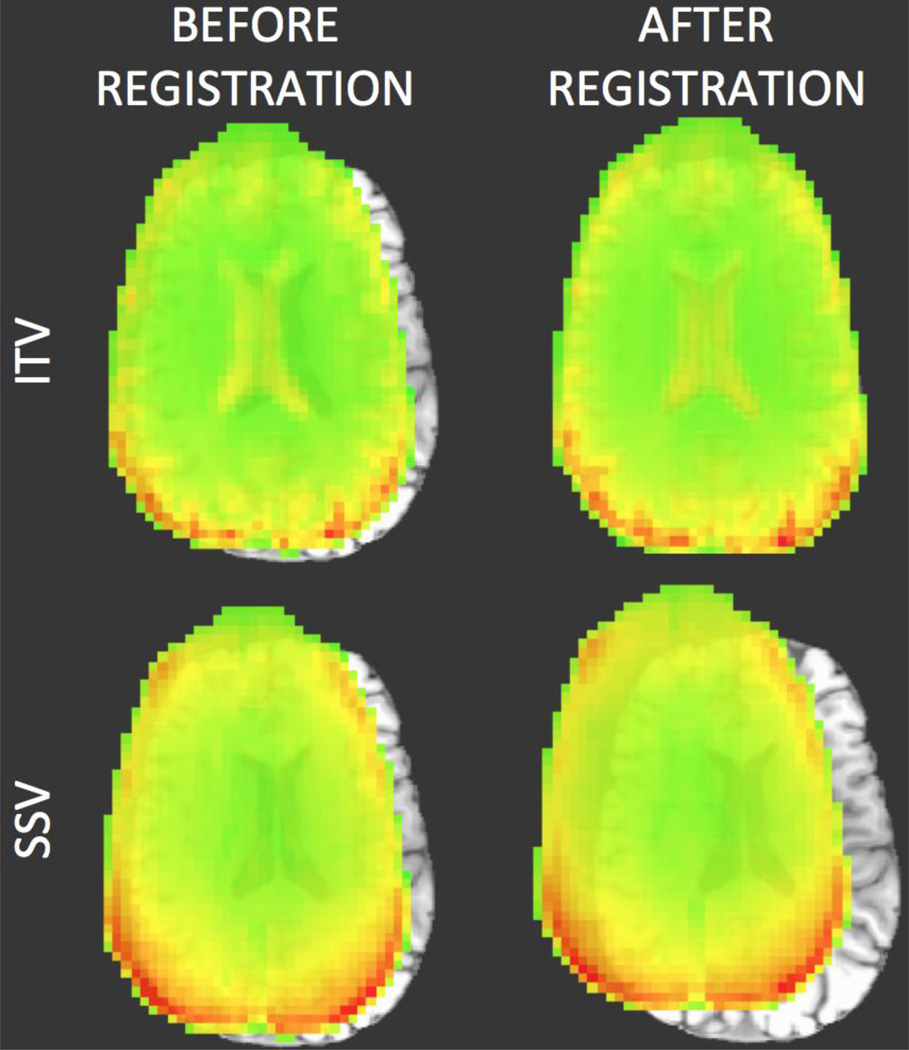
Representative case of anatomical-to-functional alignment in which alignment failed when the EPI SSV was used as the target (bottom row), but did not fail when the ITV was used as a target (top row). In all four cases, the underlay is the MPRAGE volume being aligned towards the EPI data. The overlay on the top row corresponds to the ITV prior and posterior to alignment. In the lower row the overlay corresponds to a SSV prior and posterior to alignment. In addition to the differences in the alignment results, this figure also highlights how the ITV contains higher structural information (e.g., the ventricles are clearly observed) that is not present in the SSV.

The MVD is defined as the average Euclidean distance between the position of all intra-cranial voxels subsequent to the reference alignment (i.e., when the target is the ITV) and subsequent to the alignment under consideration (e.g., when the target is the sixth volume within the functional time series). This definition results in the following mathematical formulation:

$$\mathit{\text{MVD}}=\frac{{\displaystyle {\sum }_{i=1}^N}\sqrt{{[x_{\mathit{\text{ITV}}}(i)-x_{\mathit{\text{SSV}}}(i)]}^2+{[y_{\mathit{\text{ITV}}}(i)-y_{\mathit{\text{SSV}}}(i)]}^2+{[z_{\mathit{\text{ITV}}}(i)-z_{\mathit{\text{SSV}}}(i)]}^2}}{N}$$ (Eq. 1)

where N is the number of intracranial voxels in the source volume; {x_ITV(i), y_ITV(i), z_ITV(i)} represent the coordinates in three dimensional space of each intracranial voxel (i) of the source volume after alignment towards the ITV; {x_SSV(i), y_SSV(i), z_SSV(i)} represent the coordinates of the same voxel (i) after alignment towards the SSV. Figure 2 shows a schematic of the different elements contributing to the computation of the MVD for a case of anatomical-to-functional alignment. The source volume (S)—an MPRAGE in this particular case—is shown at the top of the figure (A) in the form of an axial slice, and also as a matrix with the spatial location (x, y, z coordinates) of all intracranial voxels. Below the source, we have depicted the two targets: ITV on the left, and SSV on the right. Both of these targets in the figure correspond to EPI acquisitions at a FA of 90°. Finally, the bottom row of figure 2 shows the output for both alignments (S_ITV and S_SSV). It is the spatial coordinates of these two volumes that enter Equation 1 for the MVD calculation. Because the MVD is the average of a set of Euclidean distances between points whose location are described in mm, the unit of the MVD is mm. The interpretation of the MVD is as follows: the larger the MVD, the larger the inconsistency between the reference alignment (the one considered the gold standard) and the alignment under consideration. In the result section we provide some simulations for a known set of displacement to better characterize the behavior of the metric.

Figure 2.

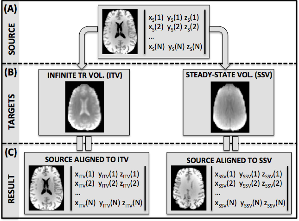
Schematic for the calculation of the Mean Voxel Distance metric (MVD) for the anatomical-to-functional scenario. Calculation of the metric involves the alignment of a source MPRAGE volume (S) to an ITV (T_ITV) and a SSV (T_SSV). For the purpose of this illustration we have considered a case of alignment of a high resolution anatomical scan (e.g., MPRAGE) to a lower resolution functional scan at a FA of 90° using data acquired with the phase-array coil.

For within-modality registration, the targets remain the same as these shown in Fig. 2.B. However the ITV is now the designated source. In order to evaluate significance of differences in MVD across scenarios, MVD results were submitted to a series of ANOVAs (see results section for details).

Registration Stability: Deviation of Mean Voxel Distance (dMVD)

Registration stability refers to the ability of an alignment algorithm to produce similar results across all possible SSV targets in an EPI time series. To quantitatively evaluate registration stability, we defined a new metric called Deviation of Mean Voxel Distance (dMVD). The dMVD is defined as the standard deviation in MVD values obtained when a given source volume is aligned to each of the SSV in a functional run.

Simulations for other TRs

TR, or time between successive acquisitions, has the potential to modulate tissue contrast in a manner similar to FA. Longer TRs are expected to increase tissue contrast because T₁ contributions at such TRs are minimized. In order to evaluate how TR affects alignment accuracy, we generated simulated data for TRs other than the one used in this experiment (TR = 2 s). Simulated data was created for each subject using the EPI signal equation by Zur et al. (1991) reproduced below (Eq. 2):

$$S=M_o·e^{-\mathit{\text{TE}}/T_2^{*}}·\frac{(1-e^{-\mathit{\text{TR}}/T_1})·\text{sin}\theta }{1-e^{-\mathit{\text{TR}}/T_1}·\text{cos}\theta }\stackrel{S_o=M_o·e^{\mathit{\text{TE}}/T_2^{*}}}{\to }S=S_o·\frac{(1-e^{-\mathit{\text{TR}}/T_1})·\text{sin}\theta }{1-e^{-\mathit{\text{TR}}/T_1}·\text{cos}\theta }$$ (Eq. 2)

where θ is the FA and S_o is the signal of the ITV for θ=90°. TR and θ were manipulated as needed. T₁ and S_o were extracted from the data. First, T₁ values were computed by means of generating T₁ maps from the EPI data using the method previously described by Bodurka et al. (2007). Second, S_o values for each tissue compartment were extracted from the ITV of the EPI acquisitions at θ=90°.

RESULTS

Evaluation of MVD Under Controlled Amounts of Displacement/Rotation

To establish the validity of the MVD as a measure of registration consistency we computed MVD for a known set of translations, rotations, and combinations of both. In particular, the initial ITV for within-modality and MPRAGE for between-modality were rotated 0°, 5°, 10°, and 15°; translated ±20.0 mm, ±12.0 mm, ±9.0 mm, ±6.0 mm, ±3.0 mm, ±2.5 mm, ±2.0 mm, ±1.5 mm, ±1.0 mm, ±0.5 mm, and 0 mm in the right/left, inferior/superior, and anterior/posterior directions; and perturbed using a combination of the four rotations and eleven translations. Figure 3 shows the results of this analysis for the anterior/posterior direction using data at θ=80° (the available angle closest to the Ernst angle for grey matter and TR=2s). Analogous results were obtained for the other directions.

Figure 3.

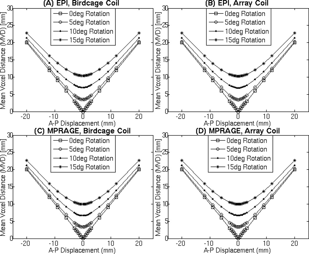
Evaluation of the MVD with datasets that have been rotated by 0° (square), 5° (triangle), 10° (circle), 15° (asterisk) and translated in the anterior/posterior direction. These MVD values were calculated from the EPI ITV acquired with the birdcage coil (A), EPI ITV acquired with the array coil (B), MPRAGE acquired with the birdcage coil (C), and MPRAGE acquired with the array coil (D). The EPI volume used for the subtraction above were acquired at a FA of 80° which is close to the Ernst Angle (θ_Ernst=77° for gray matter at 3T and TR=2s). Rotations for this analysis occurred in the A-P plane.

Intensity Bias Corrections

One factor of interest in the present work is the potential contribution of intensity inhomogeneity to errors in alignment. Before evaluating such contribution, we show in figure 4 the effect of intensity correction algorithms in all types of data under consideration. Fig. 4.A shows MPRAGE, ITV (θ=80°), and SSV (θ=80°) data acquired with the birdcage coil before and after intensity bias correction. Likewise, figure 4.B show equivalent results for the array coil. As evidenced by the bias maps (middle column on both subpanels), intensity inhomogeneity was more pronounced on the array coil data; still some inhomogeneity was present in the birdcage coil data. In the case of the array coil data, there is an evident intensity gradient from the middle of the brain towards the edges. The gradient is especially evident in the back of the brain (see white arrows in Fig. 4). In all cases, bias correction did a satisfactory job at eliminating such gradients.

Figure 4.

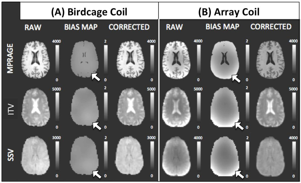
Results of the bias correction algorithm applied to the birdcage coil data (Panel A) and to the array coil data (Panel B). In each panel, the left column shows uncorrected data, the middle column shows the bias correction map, and the right column shows the corrected data. Representative data from a single subject for anatomical data (top row), EPI ITV data acquired at θ=80° (middle row), and EPI SSV data acquired at θ=80° (bottom row) is shown. White arrows indicate areas where intensity inhomogeneity was more prominent in the multi-coil data as compared to the birdcage coil data.

Registration Consistency: Qualitative Evaluation

Registration performance was first assessed visually. Figure 5 shows representative registration results for within- (Fig. 5.A) and between- (Fig. 5.B) modality registrations of data acquired with different coils and at various FAs. Visual inspection of the contours of the brain perimeter and internal brain features between S_ITV and S_SSV indicate that for within-modality there are no visually detectable differences in the alignment of the source to the SSV (Fig. 5.A). In contrast, for between-modality registrations, noticeable degradation in the quality of alignment occurs at θ=90° for registrations of data acquired with the birdcage coil, at θ≥70° for registrations of data acquired with the array coil and no correction, and at θ=90° for registrations of data acquired with the array coil that has been bias corrected. For all the aforementioned cases, the TR was 2s.

Figure 5.

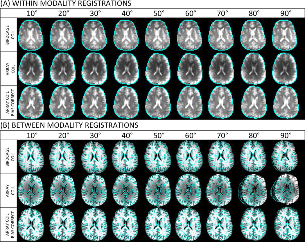
Qualitative assessment of registration accuracy for within-modality (A) and between-modality (B) registrations of uncorrected data acquired with the birdcage coil (top row), uncorrected data acquired with the array coil (middle row), and intensity inhomogeneity corrected data acquired with the array coil (bottom row). In all cases, the underlay corresponds to the source aligned to the ITV. Overlays represent single edge images of the source aligned to the SSV.

Registration Consistency: Quantitative Evaluation

Figure 6.A–B shows the MVD results for within-modality registrations before and after intensity correction of both the birdcage coil (Fig. 6.A) and the array coil (Fig. 6.B) data. The MVD increased—i.e., registration accuracy deteriorated—in both cases as FA increased. Moreover, the use of intensity correction algorithms did improve alignment results for all angles—with the exception of 10°—in both birdcage and array coil, with the improvement being more prominent in the array coil data. A 3-way mixed-effect ANOVA on the birdcage coil data ([Factor A=Subject, Random; Factor B=FA, Fixed; Factor C=Bias Correction Yes/No; Fixed]) revealed a significant main effect for FA (F=35.22; p<0.05); a significant main effect for bias correction (F=20.21; p<0.05) and a significant interaction between these two factors (F=15.88; p<0.05). Similar results were obtained for the array coil data: a significant main effect for FA (F=27.71; p<0.05), a significant main effect for bias correction (F=87.81; p<0.05); and a significant interaction between these two factors (F=49.99; p<0.05).

Figure 6.

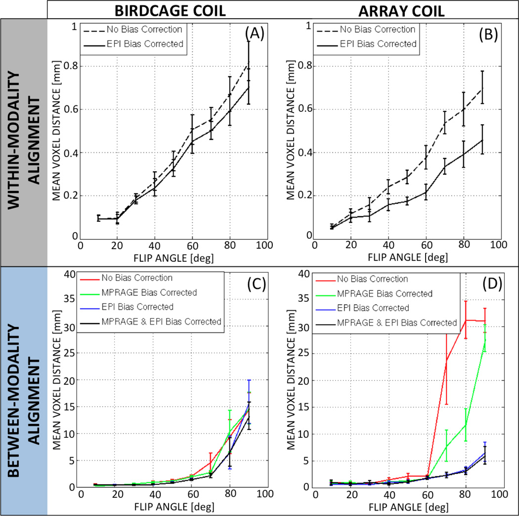
Quantitative assessment of registration consistency for within-modality registrations (A: birdcage coil & B: array coil) and between-modality registration (C: birdcage coil & D: array coil). For within-modality registration, performance was evaluated for data with no bias correction (dashed black line) and data with the bias corrected EPI (solid black line). For between-modality registration, performance was evaluated for data with no bias correction (red line), data with the raw EPI and bias-corrected MPRAGE (green line), data with the bias-corrected EPI and raw MPRAGE (blue line), and data with the bias-corrected EPI and bias-corrected MPRAGE (black line). In all cases, error bars represent standard error among subjects.

Figure 6.C–D shows the MVD results for between-modality registrations before and after intensity correction in both the birdcage coil (Fig. 6.C) and the array coil (Fig. 6.D). MVD clearly increases with FA, regardless of the bias correction scheme applied (e.g., no correction, EPI-only correction, MPRAGE-only correction, EPI & MPRAGE correction) for both coils. Comparison of Fig. 6.C and 6.D suggests that bias correction only had a clear effect on registration accuracy for data acquired with the array coil for θ>60°. A 3-way mixed-effect ANOVA (Factor A=Subject, Random; Factor B=FA, Fixed; Factor C=Correction Scheme; Fixed) on the birdcage coil data indicated a significant main effect for FA (F=16.34; p<0.05); no significant main effect for bias correction (F=2.46, p=0.09); and no significant interaction between the two factors (F=0.67, p=0.87). Conversely, the ANOVA on the array coil data indicated a significant main effect of FA (F=40.75, p<0.05); a significant main effect of bias correction (F=48.37, p<0.05); and a significant interaction between the two (F=13.49, p<0.05).

To further understand the effect of FA across the different bias correction schemes, three independent 2-ways mixed-effect ANOVAs (Factor A=Subject, Random; Factor B=FA, Fixed) were conducted. One ANOVA was conducted on the uncorrected birdcage coil data (red line in Fig. 6.C). Equivalent analyses were conducted on both the uncorrected (red line in Fig 6.D) and fully corrected (black line in Fig. 6.D) array coil datasets. Significant effects for FA were detected in all three scenarios (birdcage coil and no correction: F=11.90, p<0.05; array coil and no correction: F=20.4, p<0.05; array coil and full correction: F=7.36, p<0.05). Post-hoc pair-wise T-tests across FAs on the birdcage non-corrected data revealed significant differences (p_corrected<0.05) between the lower five angles (θ=10°, 20°, 30°, 40° and 50°) and the higher two angles (θ=80° and 90°). The same result was obtained for the uncorrected array coil data. Conversely, after bias correction, differences across FAs for the array coil data decreased with only the highest angle (90°) producing significantly worse alignment (i.e., significantly larger MVD) than the rest of the angles under consideration.

These quantitative results show substantial errors—large MVD—for several registration scenarios. The absolute magnitude of these errors can be affected by many factors including: hardware (field strength, manufacturer, RF coils, etc.), acquisition strategy (parallel acquisition strategies, parameter settings, reconstruction method, etc.) and analysis decisions (pre-processing stages, package used: AFNI/FSL/SPM, etc.). However, although the magnitude of the errors might differ across environments, the trends presented here (e.g., how alignment error varies as a function of bias field correction) are expected to be the same for all, or most, scanners, sequences and software. Therefore, the main message these results convey is about the trends, not the actual incurred errors, and how the proposed processing and acquisition changes can improve alignment.

Registration Stability: Quantitative Evaluation

Figure 7.A–B shows the dMVD for within-modality registration before and after intensity corrections in both the birdcage coil (Fig. 7.A) and array coil (Fig. 7.B). Although there are some differences across angles and across correction schemes, the dMVD is always below 0.1mm, which suggests that stability is not an issue for within-modality registration in any of the scenarios under scrutiny.

Figure 7.

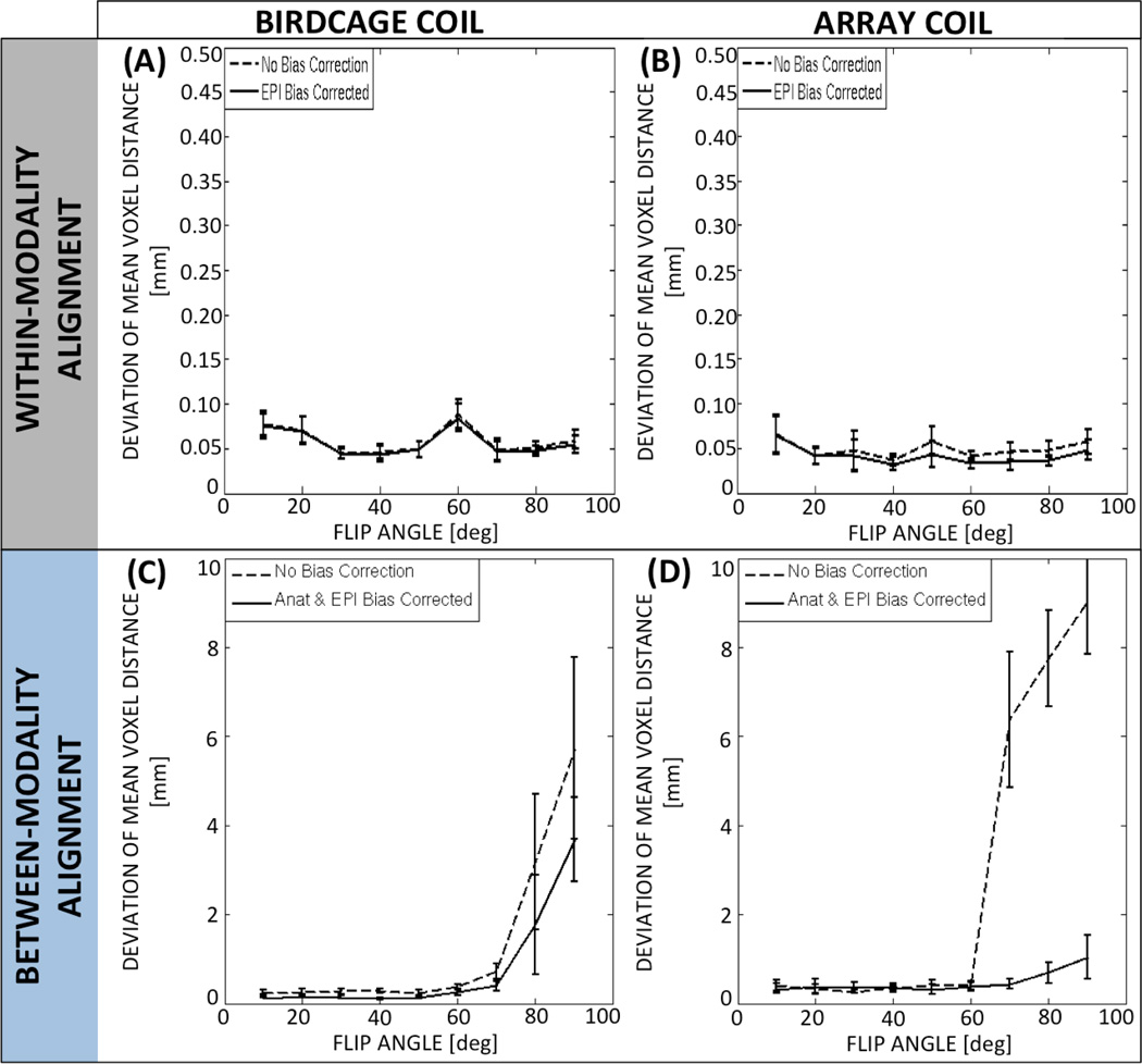
Quantitative assessment of within-modality registration (A: birdcage coil & B: array coil) and between-modality (C: birdcage coil & D: array coil) stability across FAs. Registration stability of non-corrected (dashed) and bias-corrected (solid) data is shown. Error bars indicate standard error among subjects.

Figure 7.C–D shows the dMVD for the between-modality registrations before and after intensity corrections in both the birdcage coil (Fig. 7.C) and array coil (Fig. 7.D). In contrast to the within-modality scenario, for between-modality alignment both FA and correction scheme have an important effect on the stability of the alignment. For FAs below 50°, the dMVD is less than 1mm for both coils. Still, for FAs greater than 50°, the dMVD increases substantially. This is particularly true for the non-corrected array coil data, where the dMVD reaches values above 6mm for FAs equal to or greater than 70°. The effect of correction is also clearly appreciable for high angles in the array coil data. When submitted to 3-way ANOVA, the dMVD for the birdcage coil showed a significant main effect for FA (F=7.5; p<0.05), no significant effect for correction scheme (F=3.26; p=0.11) and no significant interaction between these two factors (F=1.27; p=0.28). Conversely, for the array coil data the 3-way ANOVA revealed a significant main effect both for FA (F=23.39; p<0.05) and correction scheme (F=668.39; p<0.05), as well as a significant interaction for these two factors (F=20.38; p<0.05). Finally, when the dMVD values for the intensity corrected array coil data are submitted to a 2-way ANOVA (Factor A=Subject, Random; Factor B=FA, Fixed), it appears that the dMVD for θ≥70° is significantly greater—stability is significantly worse—than for θ<70°.

Additional TR Simulations

Figure 8.A shows axial slices at different TRs for both coils. At longer TRs (e.g., TR=4s), the contrast between the three tissue compartments is apparent with the cerebrospinal fluid (CSF) and grey matter (GM) compartments being brighter than the white matter (WM) compartment. For TR=2s and 3s contrast between these three tissue compartments is minimal; and the CSF is difficult to delineate. For shorter TRs (TR=1s), the contrast between CSF and WM reappears, but this time the contrast follows the opposite direction with the CSF being darker than the WM.

Figure 8.

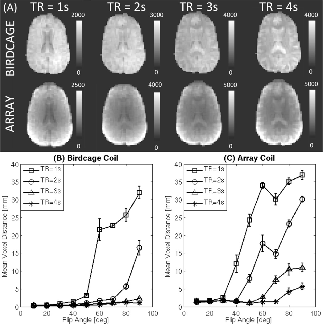
(A) Simulations of axial slices acquired at TR=1s, 2s, 3s, and 4s for both coils prior to bias correction. (B) MVD vs. FA for the birdcage coil data at different TRs (C) MVD vs. FA for the array coil data at different TRs. In both (B) and (C), longer TRs (TR≥2s) produce better alignments. Moreover, at longer TRs, differences across FAs lessen.

MVD results for between-modality registration at different TRs are shown in Fig. 8.B for the birdcage coil and in Fig. 8.C for the array coil. For the birdcage coil, at TR≥3s FA has a small effect on MVD. For TR≤2s, MVD increases—i.e., alignment worsens—for the larger angles (θ≥60°). For the array coil data, alignment worsens for larger angles at all TRs, although the worsening happens earlier—i.e., for smaller angles—and faster for the shorter TRs. A 3-way mixed-effect ANOVA ([Factor A=Subject, Random; Factor B=FA, Random; Factor C=TR, Fixed]) on the birdcage coil data shows a significant main effect for FA (F=19.85, p<0.05); a significant main effect for TR (F=38.97, p<0.05); and a significant interaction between the two (F=9.09, p<0.05). Likewise, the ANOVA on the array coil data shows a significant main effect for FA (F=44.54, p<0.05); a significant main effect for TR (F=142.04, p<0.05); and a significant interaction between the two (F=6.94, p<0.05).

DISCUSSION

In this study, we show the benefits on alignment derived from three simple-to-implement acquisition/pre-processing techniques; namely the use of low imaging FAs, correction of within-tissue intensity inhomogeneity, and the use of ITV acquisition as target volumes. The potential effect of TR in these results was also evaluated.

Evaluation of MVD metric under controlled conditions

The MVD metric was defined to quantitatively evaluate registration consistency across scenarios. To evaluate its behavior, the metric was applied to datasets that were artificially misaligned to a known distance. From the definition of the MVD and the evaluation study results (Fig. 3), we know that:

1. The MVD unit is the millimeter. Because the MVD is the average of a set of Euclidean distances measured in millimeters, the MVD unit is the millimeter (mm). In fact, figure 3 shows how the MVD for two volumes that are X mm apart in a given direction in space equals X mm. If in addition to the translation, the two volumes also differ by some degree of rotation, the MVD increases as the rotation increases.

2. The MVD is a positive monotonic function. If alignment to the target of interest is consistent with the reference target then the MVD equals zero. If alignment to the target of interest is different, then the MVD is greater than zero. Consequently, larger inconsistencies will correspond to a larger MVD, which is most likely to be due to larger misalignments.

3. The MVD is independent of intensity differences in the input. Because the input to the MVD calculation is the location of the voxels and not their intensity, the metric is independent of differences in intensity profiles across scenarios such as those derived from the use of different FAs. In other words, any difference in MVD is a result of difference in the actual location/shape of the volume after alignment, not a result of differences in intensity profiles.

FA Effects

Reduction of imaging FA in GRE-EPI helps increase tissue contrast in SSV. Our results confirm that such improved tissue contrast translates into better outcome for alignment algorithms. This is particularly true for anatomical-to-functional alignments where registration errors were easily detected by simple visual inspection (Fig 5.B). At angles 80° and above for a TR of 2s, we can see that alignment of high-resolution anatomical images towards SSV fails noticeably, especially for the array coil data. Such results were confirmed with the MVD (Fig. 6.C–D), which indicates that lower angles produce significantly better alignments than higher angles in the vicinity of the Ernst angle for both coils. One reason why alignment failed noticeably for high angles at shorter TRs is that this combination of parameters produces SSV with CSF voxels darker than WM voxels (see Figure 8) due to T1 contributions to the contrast. The LPC cost function expects CSF to be brighter than WM in the functional images, and when this assumption is violated the algorithm fails more often in the presence of intensity inhomogeneity. Other cost functions that do not assume such directionality in the contrast have the potential to perform better under these conditions (see Figure 9). In addition to that, reduction of FA also increased the stability of the alignment considerably in both coils (Fig. 7.C–D). As we shall discuss below, if data has been already acquired at these higher angles, the use of intensity inhomogeneity correction algorithms and of ITV acquisitions as target volumes constitutes solid alternatives to improve alignment results.

Figure 9.

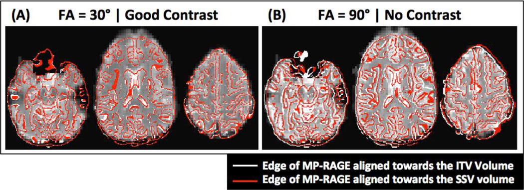
Representative results of alignment with the Border-based registration procedure (BBR). (A) Between-modality alignment of functional data with good tissue contrast (θ = 30°). (B) Between-modality alignment of functional data with poor tissue contrast (θ = 90°). In both panels the underlay corresponds to the ITV volume at the given angle, the red contour corresponds to the edges of the anatomical volume aligned towards the ITV volume, and the white contour to the edges of the anatomical volume aligned towards the SSV volume. Correspondence between these two alignments is better for the case with good tissue contrast.

For functional-to-functional registration, FA has no visually appreciable negative effects on registration (Fig. 5.A). In terms of the MVD, we found significant differences across FAs for both coils, with MVD being larger for larger angles. Still, it is worth noticing that even in the worse case the MDV was below 1mm. We believe our results indicate that the use of small FAs helps improve within- **modality alignment, but that the improvement is barely noticeable given the good consistency of alignment even for the higher angles.

As stated above, in the section devoted to quantitative assessment of registration accuracy, the magnitude of alignment errors may vary as a function of hardware, acquisition scheme and data analysis. In some cases the errors may be more subtle than here and not easily detected. Still the observation that careful selection of FA can positively influence alignment remains valid.

Intensity Inhomogeneity Correction Effects

Our results show that intensity inhomogeneity also plays a significant role in the quality and stability of alignment. The application of bias correction algorithms had a positive effect on both functional-to-functional and anatomical-to-functional alignment at high FAs, although the most noticeable effect occurs for the between-modality alignment.

Bias correction significantly improved registration consistency (e.g., reduced MVD) and stability (e.g., reduced dMVD) for anatomical-to-functional alignment in the array coil data. Three different correction approaches were tested; namely correction of EPI volumes only, correction of MPRAGE volume only, and correction of both EPI and MPRAGE volumes. All correction schemes produced some improvement in registration accuracy as compared to the case of no correction. While correction of MPRAGE data provides some benefit, the greater benefit seems to derive from correction of EPI data. In fact, figure 6.D shows that once EPI data correction is applied, additional correction of MPRAGE data does not produce any significant additional improvement. This behavior might be explained by the fact that MPRAGE data contains sufficient structural information and tissue contrast to aid with alignment prior to correction. Conversely, in EPI data, which has lower resolution and almost no contrast, structure (e.g., GM ribbon and CSF) can be identified only after bias correction.

In terms of stability, we only compared non-corrected data to fully corrected data (e.g., both EPI and MPRAGE). Stability of anatomical-to-functional alignment also improved with the application of intensity correction techniques (Fig. 7.C–D), especially for the array coil data for angles greater than 60°.

TR Effects

Repetition time is yet another acquisition parameter that affects tissue contrast. As demonstrated here, it also can affect the quality of alignment. For lower FAs (e.g., θ≤30°) TR has little effect on the outcome of alignment; as contrast is quite good across all repetition times at these lower angles. For higher angles, longer TRs are associated with better tissue contrast and consequently better alignment (i.e., lower MVD). In particular, for TR≤2s, angles greater than 70° come accompanied by deterioration of alignment as indicated by increases in MVD.

The EPI signal on a given voxel is the combined contribution of the proton density, T₁ and T₂* properties of the underlying tissue. This is clearly shown in the mathematical formulation (Eq. 2) for signal intensity in EPI (Zur et al., 1991). When TR>>T₁, the T₁ term contributes minimally to the signal independently of the FA. In the extreme case of the ITV (e.g., first EPI volume), which can be regarded as a volume acquired with an infinitely long TR, the T₁ term is eliminated from the formula. Because T₁ contributions to tissue contrast tend to cancel out differences in T₂* and proton density, when T₁ effects are not present, the tissue contrast is better. This is the case for the long TR acquisitions, in which we see that FA has little effect on the quality of the alignment.

For shorter TRs, FA modulates the contribution of the T1 term. The interaction between the T₁ exponential terms and the sine and cosine is such that lower FAs lessen the contribution of the T₁ term. As stated above, when the T₁ term highly contributes to the signal, tissue contrast degrades. This explains why at shorter TRs, the FA has a more substantial effect in the quality of the alignment. While for low FAs the T₁ term has a minimal contribution; at higher FAs, the T₁ term more heavily contributes to the signal and cancels out some of the tissue contrast originated by T₂* and proton density differences across tissues.

Recommended Strategies for Alignment

Overall, our results highlight how easy-to-implement changes in acquisition and pre-processing pipelines can produce a significant improvement in alignment. Such improvements in alignment will translate into higher quality of fMRI results and more appropriate scientific inferences. Depending on the stage at which a project is, some or all of the methods considered here can be applied. If data has already been acquired, only pre-processing steps can be implemented. If data is to be acquired, cautious selection of FA and TR can help improve tissue contrast in steady-state images.

If subjects have already been scanned, our results suggest the use of bias correction techniques prior to any alignment attempt. This is true not only for array coil data, which contain large intensity inhomogeneity that resembles the geometry of the coil elements, but also for single-element coils (e.g., the birdcage coil). Our data indicate (Fig. 4) that although intensity inhomogeneity levels on the birdcage coil data are much lower than for the array coil, there is still some level of inhomogeneity that correction algorithms can account for. Moreover, correcting such low inhomogeneity bias seems to be beneficial for alignment. If the bias correction data are not desirable in the subsequent post-processing steps, one can simply retain the transformation coordinates from the registration to the bias-corrected data and apply to the uncorrected data afterwards.

The second improvement for already acquired datasets derives from the use of ITV (e.g., first volume of the EPI series) as targets for anatomical-to-functional alignments. This first EPI ITV has significantly better contrast than the rest of the scan, and our results show that such extra contrast can help improve alignment considerably (especially if data was acquired at high FAs (e.g., θ≥60°,TR=2s). Unfortunately ITV are not always collected at the scanners. Because such volumes significantly differ from the rest of the series, they are usually eliminated during pre-processing. In some cases, they are simply discarded during acquisition. Our results suggest that whenever possible, these volumes should be collected for the sole purpose of improving alignment.

If data is to be acquired, in addition to the pre-processing considerations outlined above, careful selection of FA and TR can help bring additional improvements in tissue contrast and alignment outcome. In common practice, these two parameters are fixed based on considerations other than tissue contrast. FA is commonly selected to be equal to the Ernst angle so that signal-to-noise ratio (SNR) is maximized. Decisions on TRs usually are based on a compromise between brain coverage, spatial resolution and temporal resolution. Normally, the selected TR ends up being the shortest TR that permits acquisition of the desired number of slices at the preferred in-plane spatial resolution. Although other factors may be considered for specific studies, the criteria described above apply to most fMRI studies in cognitive neuroscience. Given the negative effects of misalignment on fMRI results, tissue contrast may be an additional factor to consider during the selection of TR and FA.

From a strictly alignment perspective, our data suggest that users should choose long TRs whenever possible. Still, long TRs are not very desirable because they translate into fewer samples per scan, which means lower temporal resolution and lower statistical power. If short TRs are selected, our data suggest choosing low FAs well below the Ernst angle. The common argument against the use of such low FAs is their detrimental effect on SNR. Although such argument is important for single-image quality, in BOLD fMRI the ultimate goal is the detection of temporal changes in the signal that correlate with the experimental paradigm. It has been recently demonstrated that when data is to be used for the purpose of BOLD activations, temporal signal-to-noise ratio (TSNR) may be a better marker of data quality (Gonzalez-Castillo et al., 2011). Moreover, in that same study, it was demonstrated that when physiological noise is the dominant source of noise in the data—which is the case for conventional 3.75×3.75×4.00 mm³ voxels at 3T—TSNR stays flat for a long range of angles above and below the Ernst angle; and, that the use of low FAs does not introduce any detrimental effect on the ability to detect BOLD activations. Additional benefits associated with the use of low FAs include improved robustness against through-plane motion artifacts, reduced physiological noise, and lower levels of heat deposition. For higher image resolution in fMRI, such as less than 2mm isometric, it may be possible for some applications (e.g., when areas with signal dropout or spatial distortion in EPI images are not considered in subsequent analyses) to rely on tissue segmentation performed directly on the EPI data and, in that way, bypass the between-modality registration step if tissue contrast is sufficient. Based on this argument, the use of low FAs for BOLD fMRI experimentation will be beneficial only at low spatial resolutions at which physiological noise constitutes the dominant source of noise in the data. According to Bodurka et al. (2007), physiological noise dominates in grey matter for voxel sizes as low as 1.8×1.8×1.8mm³ for data acquired with a 16-chanel coil on a 3T scanner—a typical hardware setup for many MRI centers around the world today.

In agreement with the previous recommendation regarding the use of low FAs, we would like to highlight one particular finding of interest. Alignment of steady-state EPI data acquired at θ≥70° towards MPRAGE data failed in a considerable number of occasions when using the LPC cost function. This is particularly true for θ=90°. The use of these angles with TRs in the range of 2–3s is very common in the literature. Our results, and experience with other datasets (not reported here), stress that such approach might not be optimal because this combination of parameters may produce SSV images with inverted or minimal contrast (i.e., CSF is darker than WM; see Figure 8), which some cost functions do not handle properly. If reduction of FA well below the Ernst angle is not feasible given available SNR and physiological noise levels—please see (Gonzalez-Castillo et al., 2011) for a complete discussion on how to decide the optimal angle to use if detection of BOLD contrast is the purpose of the study—it might still be advisable to avoid any FA above the Ernst angle given the additional deterioration of contrast that happen at these higher angles, specially at shorter TRs.

Note that the alignment between anatomical and functional images is never perfect due to different image distortions, particularly in EPI images. Additional magnetic field maps should be obtained to properly correct for the non-linear distortions in EPI images and reduce the residual misalignment. The linear registration algorithms used are incapable of correcting for such image distortions. However, the misalignment due to image distortions is independent of FA since the same EPI waveforms are applied. In some cases, like the one shown here, the distortions may be smaller than the misalignment induced by bias fields and lack of image contrast. Nevertheless, in cases where there are substantial EPI image distortions, it is advisable to perform distortion correction first using B0 field maps obtained during scanning.

Limitations of this study

One limitation of the between-modality analysis conducted in this work is that all results correspond to alignments conducted using the LPC cost function. The LPC is the default cost-function for alignment of functional and anatomical data in AFNI. It has been demonstrated to perform better than the default functions in FSL (Correlation ratio: CR) and SPM (Normalized Mutual Information: NMI) in the presence of tissue contrast. In the absence of tissue contrast, it is difficult to properly evaluate the quality of alignment, as overlap of brain edges across modalities does not necessarily ensure correct alignment of subcortical structures, ventricles or cortical folding (Saad et al., 2009). Because LPC heavily relies in tissue contrast between WM, GM and CSF to perform the alignment, it will tend to fail more dramatically than CR and NMI in terms of aligning the edges of the brain. Still, what apparently is a good alignment with CR or NMI (meaning the edges of the anatomical and the EPI overlap) may in fact be quite inaccurate, specifically for subjects with large CSF regions around the brain. Improving tissue contrast by using any of the methods described in this paper will therefore be of benefit not only for LPC users, but also for CR and NMI users.

Yet another approach to between-modality alignment is Border-Based Registration (BBR). This technique requires the creation of a surface model from the high-resolution anatomical volume prior to attempting registration. This process, when performed with the Freesurfer software (http://surfer.nmr.mgh.harvard.edu/) requires several hours of computing time. Once the surface is available, BBR uses the surface model to bring the anatomical and functional images into alignment. According to Greve and Fischl (2009), this technique is quite robust to intensity inhomogeneity. It also has the potential to perform better than LPC in low contrast situations. To obtain a preliminary understanding on how the results presented here with LPC may relate to alignment performed with BBR, we computed BBR alignment for data at two different angles with different contrasts (θ=30°, Good contrast; and θ=90°, Poor contrast) using the program bbregister (part of the Freesurfer package) and surfaces generated with Freesurfer. Figure 9 shows the results for a representative subject. The red contour corresponds to the edge of the anatomical image (AFNI 3dedge3) aligned towards the ITV volume. The white contour corresponds to the edge of the anatomical image aligned towards the SSV volume. Although BBR does not perform as poorly as LPC at aligning the borders of the brain in the poor contrast case, it is evident that consistency between alignment to the SSV and ITV degrades also for BBR when contrast is poor (red and white contour differ more for the data at θ=90° than at θ=30°). Therefore, although the benefit associated with improving tissue contrast for BBR may be lower than for LPC, BBR still can benefit from improvements in alignment derived from any of the techniques described in this manuscript.

CONCLUSIONS

Accurate and consistent alignment of functional and anatomical data is mandatory for the processing and correct interpretation of fMRI data. Here we provide three easy-to-implement recommendations to improve quality of registration: (1) use longer TRs and lower FAs whenever possible to increase tissue contrast of steady-state EPI acquisitions; (2) use intensity inhomogeneity correction algorithms for all types of data; and (3) use ITVs as targets for alignment. Moreover, we have also highlighted the detrimental effects that the use of angles higher than the Ernst angle (θ=90°) combined with relatively short TRs (TR≤2s) may have on anatomical-to-functional registrations.

Highlights.

• Spatial alignment significantly improves when tissue contrast increases.

• Low imaging angles, below the Ernst angle, provide better tissue contrast than higher angles.

• Infinite TR GRE-EPI acquisitions provide high contrast alignment targets.

• Additional improvements in alignment can be obtained by using long TRs or intensity inhomogeneity correction algorithms.

REFERENCES

- 1.Alpert NM, Berdichevsky D, Levin Z, Morris ED, Fischman AJ. Improved methods for image registration. Neuroimage. 1996;3:10–18. doi: 10.1006/nimg.1996.0002. [DOI] [PubMed] [Google Scholar]
- 2.Bartolini ME, Pekar J, Chettle DR, McNeill F, Scott A, Sykes J, Prato FS, Moran GR. An investigation of the toxicity of gadolinium based MRI contrast agents using neutron activation analysis. Magnetic Resonance Imaging. 2003;21:541–544. doi: 10.1016/s0730-725x(03)00081-x. [DOI] [PubMed] [Google Scholar]
- 3.Berry I, Chambon C, Gigaud M, Derache V, Manelfe C. Early depiction of brain ischaemia with MRI and dysprosium-dota injection. European Radiology. 1994;4:445–451. [Google Scholar]
- 4.Bodurka J, Ye F, Petridou N, Murphy K, Bandettini PA. Mapping the MRI voxel volume in which thermal noise matches physiological noise--implications for fMRI. Neuroimage. 2007;34:542–549. doi: 10.1016/j.neuroimage.2006.09.039. [DOI] [PMC free article] [PubMed] [Google Scholar]
- 5.Caravan P, Ellison JJ, McMurry TJ, Lauffer RB. Gadolinium(III) chelates as MRI contrast agents: Structure, dynamics, and applications. Chemical Reviews. 1999;99:2293–2352. doi: 10.1021/cr980440x. [DOI] [PubMed] [Google Scholar]
- 6.Cox RW. AFNI: software for analysis and visualization of functional magnetic resonance neuroimages. Comput Biomed Res. 1996;29:162–173. doi: 10.1006/cbmr.1996.0014. [DOI] [PubMed] [Google Scholar]
- 7.Davatzikos C, Prince JL, Bryan RN. Image registration based on boundary mapping. IEEE Trans Med Imaging. 1996;15:112–115. doi: 10.1109/42.481446. [DOI] [PubMed] [Google Scholar]
- 8.de Zwart JA, Ledden PJ, van Gelderen P, Bodurka J, Chu RX, Duyn JH. Signal-to-noise ratio and parallel Imaging performance of a 16-channel receive-only brain coil array at 3.0 Tesla. Magnetic Resonance in Medicine. 2004;51:22–26. doi: 10.1002/mrm.10678. [DOI] [PubMed] [Google Scholar]
- 9.Dillman JR, Ellis JH, Cohan RH, Strouse PJ, Jan SC. Frequency and severity of acute allergic-like reactions to gadolinium-containing IV contrast media in children and adults. American Journal of Roentgenology. 2007;189:1533–1538. doi: 10.2214/AJR.07.2554. [DOI] [PubMed] [Google Scholar]
- 10.Eickhoff SB, Heim S, Zilles K, Amunts K. Testing anatomically specified hypotheses in functional imaging using cytoarchitectonic maps. Neuroimage. 2006;32:570–582. doi: 10.1016/j.neuroimage.2006.04.204. [DOI] [PubMed] [Google Scholar]
- 11.Eickhoff SB, Paus T, Caspers S, Grosbras MH, Evans AC, Zilles K, Amunts K. Assignment of functional activations to probabilistic cytoarchitectonic areas revisited. Neuroimage. 2007;36:511–521. doi: 10.1016/j.neuroimage.2007.03.060. [DOI] [PubMed] [Google Scholar]
- 12.Ernst RR, Anderson WA. Application of Fourier Transform Spectroscopy to Magnetic Resonance. Review of Scientific Instruments. 1966;37:93. -+*. [Google Scholar]
- 13.Freire L, Mangin JF. Motion correction algorithms may create spurious brain activations in the absence of subject motion. Neuroimage. 2001;14:709–722. doi: 10.1006/nimg.2001.0869. [DOI] [PubMed] [Google Scholar]
- 14.Freire L, Orchard J, Jenkinson M, Mangin JF. Reducing activation-related bias in FMRI registration. Medical Imaging and Augmented Reality, Proceedings. 2004;3150:278–285. [Google Scholar]
- 15.Gholipour A, Kehtarnavaz N, Briggs R, Devous M, Gopinath K. Brain functional localization: a survey of image registration techniques. IEEE Trans Med Imaging. 2007;26:427–451. doi: 10.1109/TMI.2007.892508. [DOI] [PubMed] [Google Scholar]
- 16.Gonzalez-Castillo J, Roopchansingh V, Bandettini PA, Bodurka J. Physiological noise effects on the flip angle selection in BOLD fMRI. Neuroimage. 2011;54:2764–2778. doi: 10.1016/j.neuroimage.2010.11.020. [DOI] [PMC free article] [PubMed] [Google Scholar]
- 17.Goshtasby A. Image Registration by Local Approximation Methods. Image and Vision Computing. 1988;6:255–261. [Google Scholar]
- 18.Greve DN, Fischl B. Accurate and robust brain image alignment using boundary-based registration. Neuroimage. 2009;48:63–72. doi: 10.1016/j.neuroimage.2009.06.060. [DOI] [PMC free article] [PubMed] [Google Scholar]
- 19.Hsu CC, Wu MT, Lee C. Robust image registration for functional magnetic resonance imaging of the brain. Med Biol Eng Comput. 2001;39:517–524. doi: 10.1007/BF02345141. [DOI] [PubMed] [Google Scholar]
- 20.Jenkinson M, Bannister P, Brady M, Smith S. Improved optimization for the robust and accurate linear registration and motion correction of brain images. Neuroimage. 2002;17:825–841. doi: 10.1016/s1053-8119(02)91132-8. [DOI] [PubMed] [Google Scholar]
- 21.Jiang AP, Kennedy DN, Baker JR, Weisskoff RM, Tootell RBH, Woods RP, Benson RR, Kwong KK, Brady TJ, Rosen BR, Belliveau JW. Motion detection and correction in functional MR imaging. Human Brain Mapping. 1995;3:224–235. [Google Scholar]
- 22.Lange T, Wenckebach TH, Lamecker H, Seebass M, Hunerbein M, Eulenstein S, Gebauer B, Schlag PM. Registration of different phases of contrast-enhanced CT/MRI data for computer-assisted liver surgery planning: Evaluation of state-of-the-art methods. International Journal of Medical Robotics and Computer Assisted Surgery. 2005;1:6–20. doi: 10.1002/rcs.23. [DOI] [PubMed] [Google Scholar]
- 23.Maurer CR, Aboutanos GB, Dawant BM, Maciunas RJ, Fitzpatrick JM. Registration of 3-D images using weighted geometrical features. Ieee Transactions on Medical Imaging. 1996;15:836–849. doi: 10.1109/42.544501. [DOI] [PubMed] [Google Scholar]
- 24.Miller MI, Beg MF, Ceritoglu C, Stark C. Increasing the power of functional maps of the medial temporal lobe by using large deformation diffeomorphic metric mapping. Proceedings of the National Academy of Sciences of the United States of America. 2005;102:9685–9690. doi: 10.1073/pnas.0503892102. [DOI] [PMC free article] [PubMed] [Google Scholar]
- 25.Murphy KPJ, Szopinski KT, Cohan RH, Mermillod B, Ellis JH. Occurrence of adverse reactions to gadolinium-based contrast material and management of patients at increased risk: A survey of the American society of neuroradiology fellowship directors. Academic Radiology. 1999;6:656–664. doi: 10.1016/S1076-6332(99)80114-7. [DOI] [PubMed] [Google Scholar]
- 26.Oakes TR, Johnstone T, Walsh KSO, Greischar LL, Alexander AL, Fox AS, Davidson RJ. Comparison of fMRI motion correction software tools. Neuroimage. 2005;28:529–543. doi: 10.1016/j.neuroimage.2005.05.058. [DOI] [PubMed] [Google Scholar]
- 27.Rahman SL, Harbinson MT, Mohiaddin R, Pennell DJ. Acute allergic reaction upon first exposure to gadolinium-DTPA: a case report. Journal of Cardiovascular Magnetic Resonance. 2005;7:849–851. doi: 10.1080/10976640500288206. [DOI] [PubMed] [Google Scholar]
- 28.Roche A, Malandain G, Pennec X, Ayache N. The correlation ratio as a new similarity measure for multimodal image registration. Medical Image Computing and Computer-Assisted Intervention - Miccai'98. 1998;1496:1115–1124. [Google Scholar]
- 29.Rowland DJ, Garbow JR, Laforest R, Snyder AZ. Registration of [F-18]FDG microPET and small-animal MRI. Nuclear Medicine and Biology. 2005;32:567–572. doi: 10.1016/j.nucmedbio.2005.05.002. [DOI] [PubMed] [Google Scholar]
- 30.Saad ZS, Glen DR, Chen G, Beauchamp MS, Desai R, Cox RW. A new method for improving functional-to-structural MRI alignment using local Pearson correlation. Neuroimage. 2009;44:839–848. doi: 10.1016/j.neuroimage.2008.09.037. [DOI] [PMC free article] [PubMed] [Google Scholar]
- 31.Saeed M, Wendland MF, Masui T, Higgins CB. Reperfused myocardial infarctions on T1- and susceptibility-enhanced MRI: evidence for loss of compartmentalization of contrast media. Magn Reson Med. 1994;31:31–39. doi: 10.1002/mrm.1910310105. [DOI] [PubMed] [Google Scholar]
- 32.Samanez-Larkin GR, D'Esposito M. Group comparisons: imaging the aging brain. Social Cognitive and Affective Neuroscience. 2008;3:290–297. doi: 10.1093/scan/nsn029. [DOI] [PMC free article] [PubMed] [Google Scholar]
- 33.Schmithorst VJ, Dardzinski BJ, Holland SK. Simultaneous correction of ghost and geometric distortion artifacts in EPI using a multiecho reference scan. Ieee Transactions on Medical Imaging. 2001;20:535–539. doi: 10.1109/42.929619. [DOI] [PMC free article] [PubMed] [Google Scholar]
- 34.Thakral C, Alhariri J, Abraham JL. Long-term retention of gadolinium in tissues from nephrogenic systemic fibrosis patient after multiple gadolinium-enhanced MRI scans: case report and implications. Contrast Media & Molecular Imaging. 2007;2:199–205. doi: 10.1002/cmmi.146. [DOI] [PubMed] [Google Scholar]
- 35.Thirion B, Pinel P, Meriaux S, Roche A, Dehaene S, Poline JB. Analysis of a large fMRI cohort: Statistical and methodological issues for group analyses. Neuroimage. 2007;35:105–120. doi: 10.1016/j.neuroimage.2006.11.054. [DOI] [PubMed] [Google Scholar]
- 36.Vaquero JJ, Desco M, Pascau J, Santos A, Lee I, Seidel J, Green MV. PET, CT, and MR image registration of the rat brain and skull. Ieee Transactions on Nuclear Science. 2001;48:1440–1445. [Google Scholar]
- 37.Wells WM, 3rd, Viola P, Atsumi H, Nakajima S, Kikinis R. Multimodal volume registration by maximization of mutual information. Med Image Anal. 1996;1:35–51. doi: 10.1016/s1361-8415(01)80004-9. [DOI] [PubMed] [Google Scholar]
- 38.Zur Y, Wood ML, Neuringer LJ. Spoiling of transverse magnetization in steady-state sequences. Magnetic resonance in medicine : official journal of the Society of Magnetic Resonance in Medicine/Society of Magnetic Resonance in Medicine. 1991;21:251–263. doi: 10.1002/mrm.1910210210. [DOI] [PubMed] [Google Scholar]