Suppression of cortical neural variability is stimulus- and state-dependent

Abstract

Internally generated, spontaneous activity is ubiquitous in the cortex, yet it does not appear to have a significant negative impact on sensory processing. Various studies have found that stimulus onset reduces the variability of cortical responses, but the characteristics of this suppression remained unexplored. By recording multiunit activity from awake and anesthetized rats, we investigated whether and how this noise suppression depends on properties of the stimulus and on the state of the cortex. In agreement with theoretical predictions, we found that the degree of noise suppression in awake rats has a nonmonotonic dependence on the temporal frequency of a flickering visual stimulus with an optimal frequency for noise suppression ∼2 Hz. This effect cannot be explained by features of the power spectrum of the spontaneous neural activity. The nonmonotonic frequency dependence of the suppression of variability gradually disappears under increasing levels of anesthesia and shifts to a monotonic pattern of increasing suppression with decreasing frequency. Signal-to-noise ratios show a similar, although inverted, dependence on cortical state and frequency. These results suggest the existence of an active noise suppression mechanism in the awake cortical system that is tuned to support signal propagation and coding.

the large amount of variability commonly observed in neural responses to identical sensory stimuli across trials can obscure the relationship between neural activity and its specific external cause (de Ruyter van Steveninck et al. 1997; Softky and Koch 1993; Tolhurst et al. 1983; Vogels et al. 1989). A leading contributor to this variability is the spontaneous activity that neurons in the cortex exhibit, even in primary sensory areas, in the absence of any sensory stimulus (Arieli et al. 1996; Destexhe et al. 1999; Fiser et al. 2004; McCormick 1999). Indeed, at the behavioral level, several studies have demonstrated a correlation between high levels of spontaneous activity and poor perceptual and decision processing in awake animals and humans (Fox and Raichle 2007; Super et al. 2003). These results raise the question of how internally generated spontaneous activity and stimulus-evoked responses coexist in sensory areas without corrupting the transmission and processing of incoming information.

One possible answer to this puzzle is that stimulus-evoked activity interacts with and suppresses ongoing internally generated activity. Earlier work (Finn et al. 2007; Monier et al. 2003) and a large number of studies summarized recently (Churchland et al. 2010) indicate that intrinsically generated spontaneous fluctuations are suppressed by evoked activity throughout the cortex under a broad range of conditions. However, these results leave open an important question: if the magnitude of noise fluctuations in neural activity depends on the presence of a stimulus, does it also depend on features of the stimulus and on the state of the cortical network? A recent theoretical study (Rajan et al. 2010) showed that internally generated noise fluctuations are actively suppressed by stimulus input in generic network models and, furthermore, that the effect has an interesting dependence on the temporal frequency of the stimulus. Starting at low frequencies, noise suppression initially increases as the stimulus frequency is increased, reaches a maximum at an intermediate “optimal” frequency, and then decreases with further increases of stimulus frequency. This “resonance” effect occurs despite the fact that the spontaneous activity of the model does not show any increased power around the frequency of maximum suppression. The modeling work predicts that for periodic stimulation of fixed amplitude, neural variability should be maximally suppressed at intermediate frequencies around a few hertz even if no resonance occurs in this region of the power spectrum of the spontaneous activity (Rajan et al. 2010).

We tested this prediction and looked for state-dependent effects by recording spontaneous and visually evoked multiunit (MU) activity in the primary visual cortex (V1) of rats in awake and a range of anesthetized conditions. We found a pattern of stimulus-dependent suppression of variance that confirmed the theoretical predictions in the awake state but that shifted to a different pattern in anesthetized states. These results link the dynamics of spontaneously active recurrent neural circuits to features of sensory processing in the cortex.

MATERIALS AND METHODS

Anesthesia and recording.

We chronically implanted bundles of 16 nichrome/formvar microwires (400- to 600-kΩ impedance) attached to microdrives into V1 of adult Long-Evans rats to record extracellularly neural activity. Electrodes were implanted in V1 (stereotaxic coordinates: 6.8 mm posterior, 3.5 mm lateral to bregma) and verified to be within V1 post hoc with histological staining. Dental acrylic was used to cover the implants and support a metal head post used for later head restraint. Animals were allowed to recover from surgery, placed on a water restriction protocol, and trained to tolerate head restraint in a 8- by 4- by 6-in. Plexiglas box. Microdrives permitted periodic lowering of the electrode bundles to record from different units on different days. We recorded from 103 MU in 6 rats. Extracellular signals were filtered [154–8.8 kHz for spikes, 0.7–170 Hz for local field potentials (LFPs)] and amplified. Neural signals were digitized with a Multichannel Acquisition Processor system and sampled at 40 kHz for spikes and 1 kHz for LFPs (Plexon, Dallas, TX). All recordings were performed inside a sound- and light-attenuating chamber with flat black paint on the interior and a liquid crystal display (LCD) monitor set into one side. For awake recordings, rats sat passively viewing visual stimuli. Rats were always head-fixed to keep their eyes 6 in. in front of the monitor in the same position.

For anesthetized recordings, isoflurane was delivered with oxygen under pressure through a clear plastic mask covering the rat's nose and mouth while the rats sat in the same restraint position as in awake recordings. Isoflurane is mainly an agonist of inhibitory neurotransmitter receptors such as the GABA_A receptor (Alkire et al. 2008; Campagna et al. 2003; Rudolph and Antkowiak 2004). Rats were anesthetized at four different levels, ranging from very light to deep. To maintain different animals at the same physiological level of anesthesia, concentrations of isoflurane varied between 0.6 and 0.9% for the very light level, 0.9 and 1.2% for the light level, 1.2 and 1.6% for the medium level, and 1.6 and 2.0% for deep. Respiration rate, reflex response, and LFP structure and amplitude were recorded regularly and kept within a narrow range unique to the proper level of anesthesia for each recording session. For instance, the deep anesthesia condition was, in part, characterized by slow breathing between 44 and 48 breaths per minute, no reflex response to toe pinch, and frequent periods of silence in the LFP punctuated by short, large-amplitude, and low-frequency bursts, as commonly observed in surgical-level anesthetic conditions (Hudetz and Imas 2007; Kroeger and Amzica 2007). In contrast, very light anesthesia involved breathing rates >55 breaths per minute, strong reflex response to even light toe pinch, and continuous, small-amplitude, high-frequency oscillations in the LFPs. Very light anesthesia was close to waking in the sense that a decrease in isoflurane concentration of even 0.1–0.2% would allow the animal to start actively moving. In addition, oxygen saturation was monitored with a pulse oximeter to ensure levels stayed >93%, and body temperature was maintained between 36.7 and 37.7°C with a heating pad set into the bottom of the restraint box. Breathing, temperature, reflex response, and LFP activity were stabilized for at least 15 min at each anesthesia level before recording began to ensure standardization of levels across rats.

Recordings were made at all levels of anesthesia (and awake for restraint-habituated rats) on the same day in randomized order. Continuous recording sessions for each condition lasted ∼3 min. All anesthetized sessions were kept under 2 h in length because concentrations of inhaled anesthetics must be reduced radically after long periods of time to maintain a given level of anesthesia and because maintenance of light anesthesia and full physiological recovery from anesthesia is much more difficult after animals have been anesthetized for several hours. Animals were always allowed to wake up for at least 2 h before any awake state recordings or further administration of anesthesia. Rats underwent a second repetition of levels on a different day with a new set of units. All animal use procedures were approved by the Animal Care and Use Committee at Brandeis University.

Visual stimulation.

Stimuli were generated with Psychtoolbox software (Brainard 1997) commonly used with MATLAB (The MathWorks, Natick, MA). Full-field, square-wave, white-black flashing modulation at 100% contrast was presented on an LCD monitor set into the wall of the recording box, covering 110° of the rats' visual angle for all levels of anesthesia and waking. Recordings were made at four different conditions of visual frequency modulation, 1, 2, 3.75, and 7.5 Hz, with periods of 1.0, 0.51, 0.27, and 0.13 s, and a spontaneous condition in complete darkness with the monitor off. These conditions were presented in randomized order to eliminate possible sequence effects on the results.

Data analysis.

Waveforms that passed voltage thresholds during recording were further inspected offline for their isolation, stability over time, and low percentage of refractory spikes. Waveforms were sorted using principal components, nonlinear energy, peak-valley characteristics, as well as waveform size and shape with Offline Sorter software (Plexon). All units that collectively were separated from noise, stable over the length of the recording, and showed spike patterns that were temporally distinct from simultaneously recorded units on other electrodes were included for further analyses. Because extracellular activity on most channels was not clearly isolated from other units, activity was classified as MU. However, it is unlikely that MU consisted of more than 3 or 4 neurons. Over half of the sorted units had <2% of their waveforms within a refractory period of 2 ms, average firing rates <13 Hz, even in the awake state, and unique waveform shape and size. These facts are not consistent with MU recordings corresponding to a large number of superimposed neurons.

Units with average firing rates <1 Hz across stimulus conditions were excluded from the analysis because units with very low firing rates could not be used to measure variability across trials accurately. A total of only 9 units had to be eliminated due to low firing rates. Reduced spiking activity at high concentrations of anesthesia resulted in fewer units available for analysis at progressively deeper levels of isoflurane. A total of N = 103 units were analyzed from 6 rats (awake: n = 66, 3 rats; very light anesthesia: n = 71, 6 rats; light: n = 48, 6 rats; medium: n = 46, 6 rats; deep: n = 22, 6 rats).

Firing rates.

To determine the responsiveness of our units to visual stimulation under different conditions, we computed firing rates across trials for all units. Firing rates were computed as a function of time by passing the spike trains through a Gaussian filter, so that:

$$r\left(t\right)=\frac{1}{\sigma \sqrt{2\pi }}{\displaystyle \sum _{i=1}^N\exp \left[-\frac{1}{2}{\left(\frac{t-t_i}{\sigma }\right)}^2\right]}$$

where spike times are denoted by t_i for i = 1, 2, …, N, and σ refers to the standard deviation of the Gaussian. Rates were computed every 1 ms across the entire recording time. Firing rates defined in this way were used to examine responsiveness and for the signal-to-noise ratio calculations but not for the analysis of Fano factors, which was done with spike counts across nonoverlapping bins. The firing rate at each time point was divided by the mean firing rate of that unit to normalize responses. This was necessary to ensure that all units contributed equally to the final response measure, regardless of their overall firing rates. We computed mean-normalized firing rates over time for each unit. To do this, we divided each recording session into segments of length ∼1 s to keep the number of trials equal across conditions. Unit responses were visually inspected using autocorrelation analysis in addition to plotting the average firing rate across stimulus repetitions to verify that every condition and state showed some units with clear peaks in their firing rates at the temporal period of the visual stimulation.

Power analysis.

We calculated the power spectral densities of the LFPs and spike train data using NeuroExplorer (Plexon) and in-house MATLAB software. Briefly, for spike data, the fast Fourier transform was computed on rate histograms, and the log of the power spectral density was taken to give results in decibels with power divided into 0.1-Hz bins. To assess the power in different frequency bands, we separated the data into the five major frequency bands commonly analyzed in the literature: δ, 0–4 Hz; θ, 4–8 Hz; α, 8–12 Hz; β, 12–30 Hz; and γ, 30–70 Hz. We then plotted the power of each band as the average power across all bins within each band, after normalizing the maximum power value to 1.0 so that all spike and LFP power plots would be on the same scale. We removed a 0.5-Hz window ∼60 Hz from the γ-band to eliminate electrical artifacts. To compute power at the stimulus frequencies within the spontaneous data, we plotted the average taken from 0.5-Hz windows around each frequency of visual stimulation (1, 2, 3.75, and 7.5 Hz). We computed the power using windows between 0.2 and 1 Hz around the stimulus frequencies (data not shown) with similar results.

Analysis of variability.

Although various quantities, such as the coefficient of variation (Ditlevsen and Lansky 2011; Nawrot et al. 2008), are used to characterize the variability of neural responses across trials, we applied the commonly used Fano factor, F(T), to assess the variability in spike trains (Churchland et al. 2010). F(T) is the ratio of the variance to the mean of spike counts, n, calculated by binning the recorded spike trains into time intervals of length T, F(T) = σ_n²/<n>. Once the Fano factors were computed for each unit in a given condition (i.e., particular stimulus period and anesthetic state), we followed previous approaches (Teich et al. 1997) and fit the data to a parameterized curve F(T) as a function of T, using the equations F(T) = 1 + a$\sqrt{T}$ or F(T) = b, where a or b is a free parameter that we then used as a measure of variability describing F(T) across the full range of T. We confirmed that each parameterized curve F(T), initially calculated by least squares, provided a good fit of Fano factor data by computing the Pearson correlation coefficient between Fano factor values and the corresponding points on the fitted curves for all conditions and interval sizes.

We performed a small pilot study under light anesthesia with lower-contrast stimuli and found a qualitatively similar pattern of variability across stimulus period lengths.

Signal-to-noise ratio analysis.

Signal-to-noise ratios were computed using the firing rate r(t) for each unit across all stimulus repetitions as described in the section on firing rates above. Any particular choice of the Gaussian width (σ) in the rate filter enhanced the signal-to-noise ratio for some stimulus periods and suppressed ratios for other periods, introducing an unwanted bias. Because no value of σ is optimal for all conditions, to minimize the bias, we tested a range of values of σ for each stimulus condition in the awake state and chose a value of σ that maximized the average signal-to-noise ratio for the given stimulus condition. The σ values used were 40, 30, 20, and 10 ms for 1.0-, 0.51-, 0.27-, and 0.13-s stimulus periods, respectively. However, we found that the signal-to-noise levels and pattern across conditions were similar for other values of σ.

For signal-to-noise ratios, the signal was computed as the variance of the average of the firing rate r(t) across stimulus repetitions in a given stimulus and state condition (Lyamzin et al. 2010). The noise was calculated as the average of the variance of the firing rate across the stimulus repetitions. The signal and noise were computed across all time points without selecting any peaks or particular time points of responses at the expense of others. We calculated these values for each unit in each condition to characterize the signal-to-noise ratios for the entire recorded population.

Statistics.

Statistical analyses were performed using SPSS software (IBM) or MATLAB functions from the Statistics Toolbox (The MathWorks). To test whether each stimulus condition significantly modulated firing rates in the recorded units, we used the normalized rates averaged across time segments as described above. Visually evoked units typically had transient response peaks in all conditions (as seen in Fig. 1). Maximum response peaks for all units were temporally aligned before averaging responses across the population. The aligned peaks were then eliminated from further analysis, due to spurious enhancement of selected maxima, and the remaining segment was used to assess responsiveness. We divided these segments of the average normalized firing rates into high-firing and low-firing periods. Because responses were transient, 60-ms windows were selected around each stimulus period interval and averaged to give a response value for each unit. The average firing rates for the rest of the ∼1-s segment were assigned as the background value for each unit. A 60-ms window was set around a randomly selected time point in the spontaneous condition, and the remainder of the 1-s segment of the spontaneous activity was the background. Background values were subtracted from response values for every unit in each stimulus condition and spontaneous, and Student's paired t-tests were used to compare these response-background differences between each stimulus condition and the spontaneous condition.

Fig. 1.

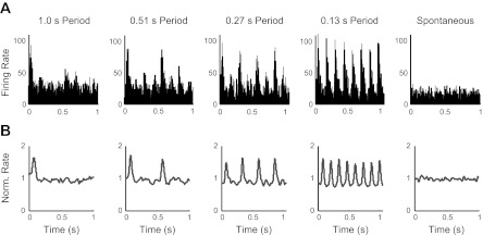
Firing rates in the awake state averaged across stimulus repetitions over ∼1-s intervals. A: firing rate histogram for 1 unit, plotted in 5-ms bins. B: average normalized (Norm.) smoothed firing rate responses (materials and methods) across all awake units (n = 66). Gray lines show the mean of the normalized rate. Peaks are present at regular stimulus-period intervals for all visual conditions, showing unit responses to the visual stimuli.

Our main tool for the remaining statistical evaluation was the ANOVA. Because we compared responses from the same neural units across different conditions, all ANOVAs applied across stimulus conditions followed a repeated-measures design, and t-tests were paired. On the basis of previous theoretical work (Rajan et al. 2010), we hypothesized that F(T) for the 0.51-s period condition would be lower than for any of the other stimulus conditions and that all stimulus conditions would have lower Fano factors than the dark spontaneous condition. We tested these general effects with repeated-measures ANOVAs across stimulus conditions. For example, to test the hypothesis that the a value for the 0.51-s stimulus period was significantly lower than for other conditions, we compared it with the average of the a values obtained using 1.0-, 0.26-, and 0.13-s stimulus periods. To test the hypothesis that variability was suppressed with visual stimulation, we compared the a values from the spontaneous condition with the average of the a values from 1.0-, 0.51-, 0.26-, and 0.13-s stimulus periods.

All further analyses on firing rates, power spectral densities, and signal-to-noise ratios were primarily to assess whether they followed similar trends as the noise suppression across stimulus conditions and states. In some cases, we compared changes across anesthesia levels. In these cases, we used one-way ANOVAs with state as the factor or two-way ANOVAs (state × stimulus) to test for a significant interaction. In some conditions, the data violated the assumption of equal variances between groups. For instance, much of the data under deeper anesthesia had lower between-unit variance than under lighter anesthesia or the awake state. In such conditions, we ran tests for unequal variances, such as Levene test of equality of error variances for across-level data or Mauchly test of sphericity for repeated-measures tests, and used corrected values, including the Greenhouse-Geisser correction, whenever necessary. The corrected values differed only slightly from standard tests and did not change the significance of any results.

RESULTS

Effect of stimulus presentation and anesthesia.

We recorded MU activity (n = 103) from V1 of 6 adult rats using full-field, square-wave, white-black flashing stimuli under 5 stimulus conditions (spontaneous and 4 frequencies, although we refer throughout to stimulus periods because this measure makes the effects we report clearer) and 5 states ranging from awake to deep anesthesia. Neural responses to the visual stimuli were 1st characterized by computing firing rate histograms across each recording session. Histograms from 1 unit in the awake state are plotted in Fig. 1A. Average responses across the population of recorded units for each state were also computed using smoothened, normalized firing rates (materials and methods). All visual conditions produced greater firing-rate modulations than the spontaneous case in the awake, very light, and light anesthetic conditions (all P < 0.001; Fig. 1B, data not shown for very light and light). Under medium and deep anesthesia, some responsiveness was lost, as has been observed previously (Ikeda and Wright 1974). This was particularly true for the shortest stimulus periods (medium: 1.0-, 0.51-, and 0.23-s periods, all P < 0.05; deep: 1.0- and 0.51-s periods, P < 0.05; other P > 0.3).

Despite the fact that periodic visual stimulation modulated firing rates, firing rates averaged across the entire recording session (∼3 min) were independent of, or at most depended weakly on, stimulus period (Fig. 2A). Only the medium and deep anesthetic states showed a significant increase in firing rate with stimulus period [repeated-measures ANOVA for stimulus period, medium: F(2.9, 129.1) = 12.1, P < 0.0001, η² = 0.212; deep: F(2.2, 45.4) = 23.8, P < 0.0001, η² = 0.531]. On the other hand, internal state, defined by the level of administered anesthesia, had a strong effect on firing. Average firing rates across stimulus conditions dropped dramatically with even the lowest concentration of isoflurane, and this reduction increased for higher concentrations of anesthetic [2-way ANOVA with state and condition as factors, state: F(24, 1,240) = 22.5, P < 0.0001, η² = 0.303; Fig. 2A]. These results are consistent with earlier findings showing qualitatively different network behavior in awake and anesthetized conditions (Fiser et al. 2004; Hudetz and Imas 2007).

Fig. 2.

General properties of the activity in awake and anesthetized states. In all plots, anesthetic states are: awake in red, very (V.) light in magenta, light in cyan, medium in green, and deep in blue. All error bars represent SE. A: average firing rates across units for all conditions and isoflurane levels. The period of the square-wave, white-black visual stimulation is given on the horizontal axis. Spontaneous activity in complete darkness is shown as single points at the left. B and C: average normalized log power spectral densities across units for the major frequency bands. Points from left to right show averages of δ- (0–4 Hz), θ- (4–8 Hz), α- (8–12 Hz), β- (12–30 Hz), and γ- (30–70 Hz) bands. B: power in spike trains. C: power in local field potentials.

To quantify the general changes across levels of anesthesia, we measured the power spectral densities of action potentials and LFPs for the spontaneous activity within different frequency bands. In agreement with previous reports (Imas et al. 2006), spike (Fig. 2B) and LFP (Fig. 2C) power decreased significantly with increased anesthesia across conditions [2-way ANOVA for state and condition, spike: F(24, 1,240) = 19.8, P < 0.0001, η² = 0.276; LFP: F(4, 295) = 29.6, P < 0.0001, η² = 0.287]. In addition, the levels of anesthesia used were distinct enough to show a significant decrease in power across bands at each successive level from awake to deep (2-way ANOVAs between neighboring states, all P < 0.05). The only exception was the LFP power between the very light and light isoflurane levels (P = 0.91). In addition, spike power across frequency bands in the awake state is flatter than under medium and deep anesthesia [significant interaction in a 2-way ANOVA with anesthesia level and frequency band as variables, F(4, 660) = 2.8, P = 0.024, η² = 0.017]. These results highlight the differences between lighter or no anesthesia vs. medium and deep anesthesia in terms of their effects on V1 activity.

Suppression of variability is stimulus-dependent.

To examine the variability of neural responses across trials, we computed the Fano factor for each unit and stimulus condition. This was done by dividing the entire recording session for each condition into time bins of size T, counting the number of spikes in each of these bins, and computing the ratio of the variance to the mean of these spike counts. Because the value of the Fano factor can depend on the size of the counting interval, we computed it over a range of intervals (T ≈ 1, 2, …, 10 s) and characterized variability using all 10 of the resulting F(T) values. In all cases, we chose counting intervals that were integer multiples of the period of the stimulus so that the pattern of visual stimulation was identical during each interval. As a result, the variability quantified by these Fano factors is not affected by fluctuations in the response that are due directly to the stimulus. Because our longest stimulus period was ∼1 s, the Fano factor intervals were never <1 s.

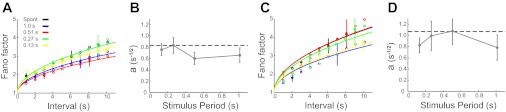
In all visually driven conditions in the awake state, as well as in the spontaneous activity, Fano factors, averaged across units, increase with spike-counting interval size, in agreement with previous reports (Rieke et al. 1997; Fig. 3A). For all counting intervals in the awake state, Fano factors were larger for spontaneous activity than in any of the stimulus-driven conditions. Furthermore, the 0.51-s period stimulus suppressed the variability, as measured by the Fano factor, more than the other stimulus frequencies. This nonmonotonic dependence of noise suppression on stimulus period was evident for all spike counting interval sizes (Fig. 3A).

Fig. 3.

Noise suppression in the awake state. All error bars represent SE, but some are eliminated in A for clarity. A: average Fano factors (circles) across all units in the awake state for different stimulus conditions and spike-counting intervals, T. Curves are fits of the Fano factor to F(T) = 1 + a$\sqrt{T}$ with different a values. Black circles and curve correspond to the spontaneous condition (Spont.); blue to the 1-s period visual stimulation; red, 0.51 s; green, 0.27 s; yellow, 0.13 s. Note that the blue curve is obscured by the red and yellow curves. B: the a values of the fits in A as a function of stimulus period, averaged across all units (n = 66). The black line represents the a value for the spontaneous data. C: F(T) vs. counting interval for 1 well-isolated single unit in the awake state. The unit demonstrates the same general trends across counting intervals and conditions as the population data in A. In this case, the black and blue curves overlap.

The points in Fig. 3A for different spike-counting intervals, in each condition, are not independent because they correspond to rebinnings of the same underlying data. The interdependence due to rebinning makes an analysis of the statistical significance of the results reported in the previous paragraph difficult. To avoid this problem while at the same time considering the results from all of the different counting intervals, we fit curves to these data and considered the mean and standard deviation of a single parameter characterizing the fitted curves.

To motivate our fits of the Fano-factor curves, it is useful to consider a conceptual model of our data. These data are most simply modeled by an inhomogeneous Poisson process, that is, a Poisson process with a time-dependent rate. The Fano factor computed across trials for a Poisson-generated spike train, even if it is inhomogeneous, is 1. However, when the Fano factor is computed by comparing the variance and mean of spike counts measured across bins over a prolonged recording session (rather than across trials for the same bin), as we do, the result deviates from 1 by an amount proportional to the variance of the underlying firing rate from bin to bin. In other words, if we define a rate for each bin by time-averaging the underlying time-dependent rate across the bin, and we compute the mean r̄ and variance σ_r²(T) of these bin-averaged rates, then F = 1 + σ_r²(T)T/r̄.

The variance σ_r²(T), which is related to the power of rate fluctuations at frequencies ∼1/T, can depend on T (Nawrot et al. 2008). We assumed a power-law dependence so that σ_r²(T)T∝T^P, and we determined the power that provided the best fit of the data in the awake state, which was P = 1/2 (Fig. 3A). Thus we fit the data with the formula F(T) = 1 + a$\sqrt{T}$, a functional form that has been used previously (Teich et al. 1997). Using this form, we fit different values of the constant a to the data for different stimulus conditions (Fig. 3B). These curves fit the Fano factor results in the awake and very light and light anesthetic conditions (see below) extremely well with Pearson correlation coefficients ranging between 0.980 and 0.93 (materials and methods).

Fits were performed for each unit separately, and Fig. 3B shows the mean and standard deviation of the resulting a values. Note that the a values we extract from MU activity may differ from the values that would be obtained from single units. Nevertheless, the $\sqrt{T}$ dependence of F(T) and the ordering of the curves for different conditions in Fig. 3A are all likely to hold for single units as well. To check this, we computed Fano factors for a randomly selected single unit that could be isolated in our recordings and found results similar to those in Fig. 3A, although, of course, noisier (Fig. 3C).

The a-parameter values used to characterize variability on the basis of fits to the Fano factors were smaller when a stimulus was present than in the spontaneous condition [repeated-measures ANOVA spontaneous vs. all stimuli: F(1, 65) = 4.8, P = 0.031, η² = 0.069; Fig. 3B]. This overall suppression is consistent with previous reports (Churchland et al. 2010). However, we also observed a dependence of the degree of suppression on the period of the stimulus. Specifically, the degree of suppression, as quantified by the decrease of the a parameter, was comparable for stimulus periods of 0.13, 0.26, and 1.0 s but significantly greater at the 0.51-s period [repeated-measures ANOVA: F(1, 65) = 5.2, P = 0.026, η² = 0.074; Fig. 3B]. Task difficulty- (Horwitz and Newsome 2001) and attention-related (Mitchell et al. 2007) suppression of low-frequency fluctuations as well as stimulus-onset-dependent suppression of variability (Churchland et al. 2010) have been found in previous analyses. However, the U-shape dependency of suppression as a function of stimulus period predicted theoretically (Rajan et al. 2010) has not been reported previously.

Suppression of variability is state-dependent.

The variability of neural responses in V1 depended strongly on the level of anesthesia. Under very light and light anesthesia, the basic characteristics of response variance were similar to those in the awake state. In both very light and light states, the change in the Fano factor across time intervals could still be captured by the 1-parameter curve, F(T) = 1 + a$\sqrt{T}$, as in the awake state (Fig. 4, A and C). The overall level of variability was somewhat smaller than in the awake state, and the amount of suppression due to the stimulus was reduced and did not reach statistical significance, with the exception of the 0.51-s period under very light anesthesia [repeated-measures ANOVA of a values: F(1, 70) = 4.9, P = 0.029, η² = 0.066; Fig. 4, B and D]. This was primarily due to a drop in the variability of the spontaneous state (compare Fig. 4, B and D, with Fig. 3B). Under very light anesthesia, the stimulus with 0.51-s period showed the maximal suppression of variability, as in the awake condition, but the effect compared with other stimulus frequencies was diminished and did not reach statistical significance (Fig. 4B). Under light anesthesia, the stimulus period dependence of the variability suppression appears to have vanished (Fig. 4D).

Fig. 4.

Variability under light anesthesia. Color scheme, fits, and error bars are as in Fig. 3. A and C: average Fano factors in the very light (A) and light (C) anesthetized states for all stimulus conditions and spike-counting intervals with their best fits (curves). B and D: the a values from the fits in A and C, respectively, plotted against the period of the visual stimulus. The black dashed line is the a value for spontaneous activity.

Under medium and deep anesthesia, the variability of the network changed qualitatively from the awake state. In these conditions, the overall levels of variability were higher than in the awake state, as has been demonstrated previously (Gur et al. 1997). Also, the Fano factor showed essentially no interval size dependence, and the 1-parameter curve F(T) = 1 + a$\sqrt{T}$ provided a poor fit (medium: Pearson r = 0.66, deep: r = 0.64). Instead, Fano factor values were fit by a constant, F(T) = b (Fig. 5, A and C), which provided a good fit (medium: r = 0.97, deep: r = 0.96), significantly better than the T-dependent fit [paired t-test of F(T) curve fit value differences; P = 0.029 and 0.014, respectively]. Furthermore, rather than exhibiting a dip across stimulus periods, the Fano factor showed a clear, monotonic decrease with increasing period, corresponding to no suppression from the level of spontaneous variability at shorter stimulus periods and increasing suppression for longer stimulus periods (reaching significance for the 0.51- and 1.0-s periods compared with spontaneous for medium: P < 0.0001 for both; and for the 1.0-s period for deep: P < 0.0001, paired t-tests; Fig. 5, B and D). This change of stimulus-period dependence could be the result of the optimal period of stimulus alternation for noise suppression having increased beyond the range explored (i.e., beyond 1 s). An increase in the optimal stimulus period is predicted in the network model if synaptic interaction strengths are decreased (Rajan et al. 2010).

Fig. 5.

Variability under deep anesthesia. Color scheme, fits, and error bars are as in Fig. 3, but the Fano factors as a function of spike-counting period T were fit to F(T) = b. A and C: average Fano factors in the medium (A) and deep (C) anesthetized states for all stimulus conditions and spike-counting intervals with their best fits (curves). B and D: the b values from the fits in A and C plotted against the period of the visual stimulus. The black dashed line is the b value for spontaneous activity. Note the different vertical axis scales for C and D relative to A and B.

The optimal period for suppression of variability does not correspond to a resonance in the power spectrum of the spontaneous activity.

A potential explanation for the pattern of suppression reported here could be the existence of a resonant frequency ∼2 Hz in the spontaneous activity that is preferentially suppressed by the 0.51-s period stimulus. This would occur if network activity were more easily entrained near this resonance and biased against entrainment at other frequencies. To rule out the possibility that the observed noise suppression for the 0.51-s period stimulus was due to a natural tendency for V1 networks to oscillate ∼2 Hz, we computed the power of the spontaneous activity, for both LFPs and spikes, in narrow bands of 0.5 Hz around each of the stimulus frequencies.

In general, the power of the spontaneous activity, measured in terms of both spike power and LFP power, showed a clear dependence on the level of anesthesia but did not reflect the period dependence of the noise suppression observed in the awake or lightly anesthetized states (Fig. 6). Unlike the Fano factor results, lighter levels of anesthesia and the awake state showed no difference in spike power between 0.51 s and the other periods [repeated-measures ANOVA for condition: awake: F(1, 65) = 0.004, P = 0.94; very light: F(1, 70) = 0.34, P = 0.56; light: F(1, 47) = 1.1, P = 0.30; Fig. 6A]. At medium and deep levels, there was a significant monotonic increase in spike power of the spontaneous activity as a function of period [repeated-measures ANOVA for condition: medium: F(1.96, 88.0) = 48.4, P < 0.0001; deep: F(2.8, 59.4) = 58.6, P < 0.0001]. The frequency dependence of the power was different for medium and deep anesthesia than for very light and light [frequency × state interaction ANOVA, F(3, 740) = 3.1, P = 0.026] or for awake [F(3, 528) = 3.0, P = 0.029; Fig. 6A]. Similar trends were observed in LFP power with no evidence of a resonance, except that in the awake and lightly anesthetized states, the spontaneous power spectrum was flat for spikes (Fig. 6A) and slowly rising for LFPs (Fig. 6B) over the range of stimulus periods studied.

Fig. 6.

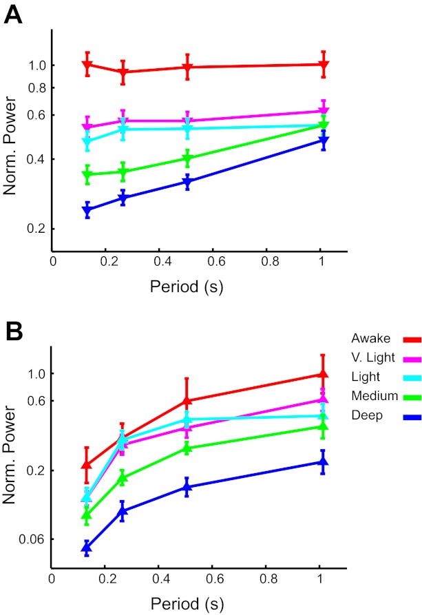
Power in the spontaneous activity at frequencies corresponding to the stimulus periods. The color scheme is the same as in Fig. 2. All error bars represent SE. A: average normalized log power for unit spiking plotted against the period being analyzed. B: average normalized log power for local field potentials.

These results suggest that resonance frequencies in the internally generated activity cannot account for the pattern of noise suppression across stimulus frequencies observed in the awake and very lightly anesthetized states (Figs. 3 and 4). In these states, the data do not show any prominent peaks around the period when maximal suppression occurs. In contrast, the monotonic increase in spontaneous power as a function of period (Fig. 6A) could provide a basis for the increased suppression of variability with stimulus period seen in medium and deep states of anesthesia (Fig. 5).

Signal-to-noise ratios.

To this point, we have concentrated on the noise component of the visual response, not on the mean response reflecting the signal. We now include this latter component by considering signal-to-noise ratios. Signal-to-noise ratios were quite small, sometimes <0.1. This is likely due to the fact that neurons in this study, which was based on chronically implanted electrode bundles, were not selected for being strongly responsive, and the stimuli were not tuned either spatially or temporally to maximize responses. Although these signal-to-noise ratios were relatively small, they were much greater than even the largest corresponding ratios obtained from the spontaneous activity [repeated-measures ANOVA spontaneous vs. all stimuli in awake state: F(1, 65) = 47.4, P = 2 × 10⁻⁹, η² = 0.42], confirming that firing rates were significantly modulated by the periodic stimuli (Fig. 7).

Fig. 7.

Signal-to-noise ratios. All error bars represent SE. The color scheme is the same as in Fig. 2. A: average signal-to-noise ratios in the awake state as a function of stimulus period. B: average signal-to-noise ratios in various states of anesthesia vs. stimulus period. Black circles in both plots represent spontaneous signal-to-noise ratios, computed with the same intervals as each stimulus period above it.

The signal-to-noise ratios show similar stimulus and state dependence as the Fano factor results but in the opposite direction. In the awake state, the signal-to-noise ratio reaches a maximum at the 0.51-s period stimulus compared with the average of the 1.0, 0.27, and 0.13-s period conditions [repeated-measures ANOVA: F(1, 65) = 4.4, P = 0.04, η² = 0.063], which is at the same stimulus period when Fano factors are maximally suppressed. Consistent with the results of variability suppression, the pattern of signal-to-noise ratios across stimulus conditions changed from awake to anesthetized recordings (Fig. 7B). Under anesthesia, signal-to-noise ratios showed a monotonic relationship to stimulus period, inverse to the variability results found under deeper anesthesia (Fig. 5). However, unlike the variability (compare Figs. 4 and 5), the signal-to-noise ratios steadily increased with the stimulus period even for the very light to light levels of anesthesia, suggesting that signal responses to higher-frequency stimuli may be modified by even small concentrations of anesthetic.

DISCUSSION

One of our novel findings is that, in the awake animal, the suppression of spontaneous variability depends on the frequency of a sensory stimulus in a nonmonotonic manner. The optimal frequency of noise suppression was observed to be ∼2 Hz, and this did not correspond to any resonant feature in the power spectrum of the spontaneous activity. A second finding is that this specificity is not maintained when the animal transitions from awake to anesthetized states. A third related finding is that the dependence of F(T) on spike-counting interval changes from square root to constant under medium and deep anesthesia. Together, these results expand our understanding of the relationship between spontaneous and visually evoked activities in both awake and anesthetized conditions.

Fano factors are often measured in time periods of 100–1,000 ms and have been computed from data collected under widely varying conditions, including different layers of the cortex, in anesthetized and awake preparations, with or without control of eye movements, for different counting interval sizes, and with stimuli presented either continuously or with sudden onset. The resulting Fano factors vary widely from sub- to supra-Poisson levels (Gershon et al. 1998; Gur et al. 1997; Kara et al. 2000; Vogel et al. 2006). In this study, we focused on aspects of variability that apply across interval sizes and persist over random sampling across cortical layers. Although the Fano factor values may vary across preparations and studies, our main results showing stimulus-selective suppression of variability and different interval dependence in the awake and anesthetized conditions are likely to be more general.

Previous studies have shown that stimulus onset reduces the variability of the neural signal in many cortical areas regardless of whether the animal is anesthetized or awake and independent of the task being performed in the awake state (Churchland et al. 2010). The reduction of variability can be detected both at the level of membrane potentials and, after appropriate controls, in extracellular recordings. Other factors, such as modulation of attention (Cohen and Maunsell 2009; Mitchell et al. 2007), could contribute to the reduction of variance, but its widespread nature suggests that the phenomenon may be a general network property (Churchland et al. 2010). In the present study, we extend previous findings by showing that suppression depends on the temporal frequency of the stimulus in the awake state in a manner consistent with theoretical predictions (Rajan et al. 2010), which supports the idea that stimulus-dependent variance suppression is a general network phenomenon. In addition, we found that this stimulus dependence is not preserved when the animal is anesthetized.

The changes in results with increasing anesthesia are marked by several apparently distinct shifts. They do not all occur at the same state transition, suggesting that several independent aspects of the network have varying sensitivity to anesthesia. First, as the animal shifts from waking to very light anesthesia, signal-to-noise ratios drop off at shorter stimulus frequencies, following the same pattern as the power spectra. In addition, the noise suppression with visual stimulation is reduced. As anesthesia is increased further from very light to light levels, the dip in variability ∼2 Hz disappears entirely, suggesting that this property of the network might operate independently from the general suppression of variability with stimulus onset, which has been observed previously. At even higher concentrations of anesthesia, the frequency dependence of the suppression shifts to a monotonic pattern favoring the lowest frequencies of visual stimulation. The dependence of the Fano factor on the counting interval is also lost, meaning that unit activity is highly variable even at short time scales. This may be indicative of a simpler temporal structure of V1 activity under deeper anesthesia as well as of the gradual shift to lower frequencies with increasing inhibition, which may be general property of anesthesia (Erchova et al. 2002).

Signal-to-noise ratios generally reflect the inverse of the variability suppression, suggesting that the 0.51-s period may be preferred from a signal processing standpoint. Although there is a peak at 0.51-s period, there is less variation in the signal-to-noise values over period lengths in the awake state than under any level of anesthesia (compare maximum and minimum values for Fig. 7, A vs. B). In particular, the values in the awake state are never as low as they get under anesthesia. We speculate that despite some significant variability across stimuli, this relative balance in the awake state could be useful for sensory processing.

This interpretation assumes that spontaneous activity corresponds to unwanted noise in the system. An alternative functional interpretation of spontaneous activity has been proposed recently based on normative considerations about the requirements of optimal internal representations in the cortex (Berkes et al. 2011). According to this proposal, the cortex approximates probabilistic inference and learning when processing sensory inputs, and spontaneous activity is not noise but represents the prior information of the network based on the internally stored model and on knowledge of the outside world. The internal model itself is represented in the structure of the cortical network, including the connectivity and the synaptic strengths within and across areas (Ringach 2009). In this framework, spontaneous activity is incorporated into the stimulus-dependent activity. Although this is a different interpretation from the mechanistic suppression based on network properties, the two might not be mutually exclusive. The normative model provides a view of how computations related to particular experience could be carried out in the cortex without specifying the exact neural computations necessary, whereas the network model offers a powerful general computational tool without defining what needs to be computed and why. Further combined experimental and theoretical work is necessary to examine whether the active noise-suppression mechanism found in the present study is a special case of a more general information processing framework in cortical networks.

GRANTS

This study was sponsored by National Eye Institute Grant EY-018196, the National Science Foundation Grant IOS 1120938, and the Swartz Foundation. L. F. Abbott was supported by the Swartz, Gatsby, and Kavli Foundations and National Institute of Mental Health Grant 093338.

DISCLOSURES

No conflicts of interest, financial or otherwise, are declared by the author(s).

AUTHOR CONTRIBUTIONS

J.F. conceived the experiment and design; B.W. and J.F. designed the study; B.W. performed experiments; B.W. and L.F.A. analyzed data; B.W., L.F.A., and J.F. interpreted results and wrote the manuscript.

REFERENCES

- Alkire MT, Hudetz AG, Tononi G. Consciousness and anesthesia. Science 322: 876–880, 2008 [DOI] [PMC free article] [PubMed] [Google Scholar]
- Arieli A, Sterkin A, Grinvald A, Aertsen A. Dynamics of ongoing activity: explanation of the large variability in evoked cortical responses. Science 273: 1868–1871, 1996 [DOI] [PubMed] [Google Scholar]
- Berkes P, Orbán G, Lengyel M, Fiser J. Spontaneous cortical activity reveals hallmarks of an optimal internal model of the environment. Science 331: 83–87, 2011 [DOI] [PMC free article] [PubMed] [Google Scholar]
- Brainard DH. The Psychophysics Toolbox. Spat Vis 10: 443–446, 1997 [PubMed] [Google Scholar]
- Campagna JA, Miller KW, Forman SA. Mechanisms of actions of inhaled anesthetics. N Engl J Med 348: 2110–2124, 2003 [DOI] [PubMed] [Google Scholar]
- Churchland MM, Yu BM, Cunningham JP, Sugrue LP, Cohen MR, Corrado GS, Newsome WT, Clark AM, Hosseini P, Scott BB, Bradley DC, Smith MA, Kohn A, Movshon JA, Armstrong KM, Moore T, Chang SW, Snyder LH, Lisberger SG, Priebe NJ, Finn IM, Ferster D, Ryu SI, Santhanam G, Sahani M, Shenoy KV. Stimulus onset quenches neural variability: a widespread cortical phenomenon. Nat Neurosci 13: 369–378, 2010 [DOI] [PMC free article] [PubMed] [Google Scholar]
- Cohen MR, Maunsell JH. Attention improves performance primarily by reducing interneuronal correlations. Nat Neurosci 12: 1594–1600, 2009 [DOI] [PMC free article] [PubMed] [Google Scholar]
- de Ruyter van Steveninck RR, Lewen GD, Strong SP, Koberle R, Bialek W. Reproducibility and variability in neural spike trains. Science 275: 1805–1808, 1997 [DOI] [PubMed] [Google Scholar]
- Destexhe A, Contreras D, Steriade M. Spatiotemporal analysis of local field potentials and unit discharges in cat cerebral cortex during natural wake and sleep states. J Neurosci 19: 4595–4608, 1999 [DOI] [PMC free article] [PubMed] [Google Scholar]
- Ditlevsen S, Lansky P. Firing variability is higher than deduced from the empirical coefficient of variation. Neural Comput 23: 1944–1966, 2011 [DOI] [PubMed] [Google Scholar]
- Erchova IA, Lebedev MA, Diamond ME. Somatosensory cortical neuronal population activity across states of anaesthesia. Eur J Neurosci 15: 744–752, 2002 [DOI] [PubMed] [Google Scholar]
- Finn IM, Priebe NJ, Ferster D. The emergence of contrast-invariant orientation tuning in simple cells of cat visual cortex. Neuron 54: 137–152, 2007 [DOI] [PMC free article] [PubMed] [Google Scholar]
- Fiser J, Chiu CY, Weliky M. Small modulation of ongoing cortical dynamics by sensory input during natural vision. Nature 431: 573–578, 2004 [DOI] [PubMed] [Google Scholar]
- Fox MD, Raichle ME. Spontaneous fluctuations in brain activity observed with functional magnetic resonance imaging. Nat Rev Neurosci 8: 700–711, 2007 [DOI] [PubMed] [Google Scholar]
- Gershon ED, Wiener MC, Latham PE, Richmond BJ. Coding strategies in monkey V1 and inferior temporal cortices. J Neurophysiol 79: 1135–1144, 1998 [DOI] [PubMed] [Google Scholar]
- Gur M, Beylin A, Snodderly DM. Response variability of neurons in primary visual cortex (V1) of alert monkeys. J Neurosci 17: 2914–2920, 1997 [DOI] [PMC free article] [PubMed] [Google Scholar]
- Horwitz GD, Newsome WT. Target selection for saccadic eye movements: prelude activity in the superior colliculus during a direction-discrimination task. J Neurophysiol 86: 2543–2558, 2001 [DOI] [PubMed] [Google Scholar]
- Hudetz AG, Imas OA. Burst activation of the cerebral cortex by flash stimuli during isoflurane anesthesia in rats. Anesthesiology 107: 983–991, 2007 [DOI] [PubMed] [Google Scholar]
- Ikeda H, Wright MJ. Sensitivity of neurones in visual cortex (area 17) under different levels of anaesthesia. Exp Brain Res 20: 471–484, 1974 [DOI] [PubMed] [Google Scholar]
- Imas OA, Ropella KM, Wood JD, Hudetz AG. Isoflurane disrupts anterio-posterior phase synchronization of flash-induced field potentials in the rat. Neurosci Lett 402: 216–221, 2006 [DOI] [PubMed] [Google Scholar]
- Kara P, Reinagel P, Reid RC. Low response variability in simultaneously recorded retinal, thalamic, and cortical neurons. Neuron 27: 635–646, 2000 [DOI] [PubMed] [Google Scholar]
- Kroeger D, Amzica F. Hypersensitivity of the anesthesia-induced comatose brain. J Neurosci 27: 10597–10607, 2007 [DOI] [PMC free article] [PubMed] [Google Scholar]
- Lyamzin DR, Macke JH, Lesica NA. Modeling population spike trains with specified time-varying spike rates, trial-to-trial variability, and pairwise signal and noise correlations. Front Comput Neurosci 4: 144, 2010 [DOI] [PMC free article] [PubMed] [Google Scholar]
- McCormick DA. Developmental neuroscience. Spontaneous activity: signal or noise? Science 285: 541–543, 1999 [DOI] [PubMed] [Google Scholar]
- Mitchell JF, Sundberg KA, Reynolds JH. Differential attention-dependent response modulation across cell classes in macaque visual area V4. Neuron 55: 131–141, 2007 [DOI] [PubMed] [Google Scholar]
- Monier C, Chavane F, Baudot P, Graham LJ, Fregnac Y. Orientation and direction selectivity of synaptic inputs in visual cortical neurons: a diversity of combinations produces spike tuning. Neuron 37: 663–680, 2003 [DOI] [PubMed] [Google Scholar]
- Nawrot MP, Boucsein C, Molina VR, Riehle A, Aertsen A, Rotter S. Measurement of variability dynamics in cortical spike trains. J Neurosci Methods 169: 374–390, 2008 [DOI] [PubMed] [Google Scholar]
- Rajan K, Abbott LF, Sompolinsky H. Stimulus-dependent suppression of chaos in recurrent neural networks. Phys Rev E Stat Nonlin Soft Matter Phys 82: 011903, 2010 [DOI] [PMC free article] [PubMed] [Google Scholar]
- Rieke F, Warland D, de Ruyter van Stevenick R, Bialek W. Spikes: Exploring the Neural Code. Cambridge, MA: MIT Press, 1997 [Google Scholar]
- Ringach D. Spontaneous and driven cortical activity: implications for computation. Curr Opin Neurobiol 19: 439–444, 2009 [DOI] [PMC free article] [PubMed] [Google Scholar]
- Rudolph U, Antkowiak B. Molecular and neuronal substrates for general anaesthetics. Nat Rev Neurosci 5: 709–720, 2004 [DOI] [PubMed] [Google Scholar]
- Softky WR, Koch C. The highly irregular firing of cortical cells is inconsistent with temporal integration of random EPSPs. J Neurosci 13: 334–350, 1993 [DOI] [PMC free article] [PubMed] [Google Scholar]
- Super H, van der Togt C, Spekreijse H, Lamme VA. Internal state of monkey primary visual cortex (V1) predicts figure-ground perception. J Neurosci 23: 3407–3414, 2003 [DOI] [PMC free article] [PubMed] [Google Scholar]
- Teich MC, Heneghan C, Lowen SB, Ozaki T, Kaplan E. Fractal character of the neural spike train in the visual system of the cat. J Opt Soc Am A 14: 529–546, 1997 [DOI] [PubMed] [Google Scholar]
- Tolhurst DJ, Movshon JA, Dean AF. The statistical reliability of signals in single neurons in cat and monkey visual-cortex. Vision Res 23: 775–785, 1983 [DOI] [PubMed] [Google Scholar]
- Vogel EK, Woodman GF, Luck SJ. The time course of consolidation in visual working memory. J Exp Psychol Hum Percept 32: 1436–1451, 2006 [DOI] [PubMed] [Google Scholar]
- Vogels R, Spileers W, Orban GA. The response variability of striate cortical neurons in the behaving monkey. Exp Brain Res 77: 432–436, 1989 [DOI] [PubMed] [Google Scholar]