Separate Magnitude and Phase Regularization via Compressed Sensing

Abstract

Compressed sensing (CS) has been used for accelerating magnetic resonance imaging (MRI) acquisitions, but its use in applications with rapid spatial phase variations is challenging, e.g., proton resonance frequency shift (PRF-shift) thermometry and velocity mapping. Previously, an iterative MRI reconstruction with separate magnitude and phase regularization was proposed for applications where magnitude and phase maps are both of interest, but it requires fully sampled data and unwrapped phase maps. In this paper, CS is combined into this framework to reconstruct magnitude and phase images accurately from undersampled data. Moreover, new phase regularization terms are proposed to accommodate phase wrapping and to reconstruct images with encoded phase variations, e.g., PRF-shift thermometry and velocity mapping. The proposed method is demonstrated with simulated thermometry data and in-vivo velocity mapping data and compared to conventional phase corrected CS.

I. Introduction

In most MRI applications, only the voxel magnitudes are of interest. However, in applications like field map estimation [1] and phase contrast imaging [2] [3], phase maps also contain important information and need to be accurately estimated. Therefore, we want to reconstruct images with both accurate magnitude and phase components from raw k-space data. Regularized iterative algorithms can reconstruct complex images with certain regularization terms for complex unknowns (the unknown image) based on certain priors, e.g., piece-wise smoothness (Total Variation [4]). Such priors, however, are usually based on properties of the magnitude component of medical images, and may be less suitable when variation of the phase component over space is not negligible. Meanwhile, such reconstructions may not exploit prior knowledge of the phase image which is often different from that of the magnitude image, causing the Signal to Noise Ratio (SNR) of phase image in low magnitude areas to be extremely low. To solve this problem, Fessler et al. proposed an iterative reconstruction method [5] in which the phase and the magnitude images are regularized for their own features separately, preserving both smoothness of the phase image and resolution of the magnitude image. However, this method cannot handle big jumps in wrapped phase maps, due to non-convexity of the cost function for the phase. Moreover, we have found that when k-space data are undersampled, Compressed Sensing (CS) methods [6] are more effective than the simpler smoothness or edge-preserving regularizers for the magnitude component considered in [5].

Undersampling k-space data is one of the main ways to accelerate MRI acquisitions, e.g., in parallel imaging and in CS. CS has shown good performance in reducing k-space samples by exploiting sparsity of medical images in certain transform domains, e.g., finite differences and wavelet transforms. However, typically the assumption of sparsity is based on the properties of the magnitude component, and CS may not work well when rapid spatial phase variations exist. To mitigate this problem, CS reconstruction methods often use phase estimation [6] to make phase corrected images so that the phase variations are reduced, making images sparser; such estimation is done by acquiring low frequency regions of k-space. A similar idea was introduced in the partial Fourier partially parallel imaging technique [7] which is based on conjugate symmetry in k-space for real images [8]. In that method, the phase corrected image is supposed to be almost real, so its imaginary component’s energy is constrained to be very low. The performance of both methods relies on a phase map estimation that may require additional acquisition and may not be accurate enough. Meanwhile, such estimation is based on the fact that phase map is spatially smooth, which might not be true in certain applications, e.g., in PRF-shift thermometry [2] and in phase-contrast velocity mapping [3]. In fact, it is contradictory that in the cases when phase correction is most necessary, i.e., rapid spatial phase variation, it is most difficult to estimate phase accurately from low frequency k-space data. Thus, phase correction may not greatly benefit magnitude reconstruction when phase variation is severe. Furthermore, since only low frequency k-space measurements are used, neither of those methods can reconstruct details in phase images, such as hot spots in thermometry and high velocity arteries in velocity mapping.

Therefore, it is tempting to extend the idea of using separate regularization of the magnitude and phase components by using CS, to improve the reconstruction of both magnitude and phase images while accelerating data acquisitions by undersampling k-space data. This combination theoretically takes advantages of these two techniques by exploiting sparsity of magnitude component and smoothness (or some other features) of phase component. Thus, Zibetti et al. proposed new regularization terms to approximate CS regularizer (l₁ norm) for magnitude and first-order roughness penalty for phase in [9], which showed better results than before. This method, however, has several limitations: first, it is only applicable for first-order differences operator in CS regularization, which is usually not the optimal one; second, the phase regularization term is still weighted by its corresponding magnitude, which may cause low SNR in low magnitude areas, in other words, phase is still not regularized independently from magnitude; last, the penalty function for phase is concave when neighboring phase difference is large, e.g., [ $\frac{\pi }{2},\frac{3\pi }{2}$], which requires a good initialization for phase.

We propose a reconstruction method that combines CS with separate regularizations for magnitude and phase for more general MRI reconstruction applications. In the framework of the separate regularization in [5], we apply CS regularization for the magnitude image but use a new phase regularizer that is applicable for wrapped phase maps, and we randomly undersample k-space data. Since this framework is general enough to design different regularizers for specific types of phase maps, we developed another type of phase regularizer for applications that have distinct areas on top of smooth background in the phase map, e.g., hot spots in temperature maps and arteries in velocity maps.

In this paper, we start with the basic MRI signal model. Then the reconstruction cost functions are discussed in detail by comparing conventional CS method with our proposed method and introducing new phase regularizers with their properties. Next, we discuss the respective optimization algorithms for magnitude and phase. Finally, the proposed method was tested by comparing with conventional phase-corrected CS in both simulation studies and in-vivo data reconstructions; in the simulation studies, we simulated an abdomen thermometry data with hot spots in the phase map; in the in-vivo data reconstruction, we acquired velocity mapping data of the abdominal aorta by a phase-contrast bSSFP sequence on 3T GE scanner.

II. THEORY

A. Signal Model

In this paper, we only discuss single coil reconstruction, but the algorithms easily generalize to parallel imaging using sensitivity encoding (SENSE) [11]. The baseband signal equation of MRI is the following:

$$s(t)=\int m(\overrightarrow{r})e^{-ix(\overrightarrow{r})}{e}^{-i2\pi \overrightarrow{k}(t)·\overrightarrow{r}}d\overrightarrow{r}$$ (1)

where r⃗ is the coordinate in spatial domain, m(r⃗) is the object “magnitude”, x(r⃗) is the phase map, and k⃗(t) is the k-space trajectory. We allow m(r⃗) to take negative values to avoid any π jumps aborbed into the phase x(r⃗). We assume a short data acquisition time so that the off-resonance induced phase is contained in x(r⃗). In MRI scanning, complex Gaussian modeled random noise ε(t) is involved in the detected signal, which is:

$$y(t)=s(t)+\epsilon (t)$$ (2)

where y(t) is the detected signal. For computation, we discretize the signal equation as follows:

$$\mathit{y}=A({\mathit{m}e}^{i\mathit{x}})+\mathit{\epsilon }$$ (3)

where y = [y₁, y₂, …, y_Nd]^T ∈ ℂ^N_d, are the measured data; A ∈ ℂ^N_d*N_p is the system matrix of MRI, e.g., the discrete Fourier transform (DFT) matrix, m = [m₁, m₂, …, m_Np]^T ∈ ℝ^N_p is the magnitude image, x = [x₁, x₂, …, x_Np]^T ∈ ℝ_Np is the phase image, and ε = [ε₁, ε₂, …, ε_Nd] ∈ ℂ^N_d is the complex noise. (We write me^ix as as shorthand for element-wise multiplication of these two vectors.) In this paper, our goal is to reconstruct m and x simultaneously from undersampled k-space data y.

B. Cost Functions

In conventional CS [6], applying a regularized approach for (3) yields the cost function:

$${\mathrm{\Psi }}_0(\mathit{f})={\left|\right|\mathit{y}-A\mathit{f}\left|\right|}^2+\beta R(\mathit{f})$$ (4)

where f = me^ix, y denotes randomly undersampled data in k-space, ||·|| denotes l₂ norm, β is the scalar regularization parameter, and R(·) is the CS regularizer; usually, R(·) is the l₁ or l₀ norm of finite differences or a wavelet transform. The estimated magnitude and phase, i.e., m̂ and x̂ are then computed from the reconstructed complex image f̂, where f̂ = argmin_f Ψ₀(f).

To reduce phase variation of f, phase-correction is often applied to better sparsify the image f in the sparse transform domain [6]:

$${\mathrm{\Psi }}_1({\mathit{f}}_1)={\left|\right|\mathit{y}-{Ae}^{i\mathit{P}}{\mathit{f}}_1\left|\right|}^2+\beta R({\mathit{f}}_1)$$ (5)

where P is the estimated phase map from low frequency k-space, e^iP denotes a diagonal matrix whose diagonal entries are exponentials of P in the same order. The unknown f₁ should then be closer than f in (4) to the magnitude image m which is sparser. The final reconstructed image for conventional CS is:

$$\widehat{\mathit{f}}=e^{i\mathit{P}}{\widehat{\mathit{f}}}_1,\widehat{\mathit{m}}=\mid \widehat{\mathit{f}}\mid ,\widehat{\mathit{x}}=\angle \widehat{\mathit{f}}$$ (6)

where f̂₁ = argmin_f1 Ψ₁(f₁).

In this paper, this method is used for comparison, and we choose R(·) to be l₁ norm of wavelet transform; then the cost function becomes:

$${\mathrm{\Psi }}_1({\mathit{f}}_1)={\left|\right|\mathit{y}-{Ae}^{i\mathit{P}}{\mathit{f}}_1\left|\right|}^2+\beta {\left|\right|U^{\prime }{\mathit{f}}_1\left|\right|}_1$$ (7)

where U is the wavelet transform matrix and ||·||₁ denotes l₁ norm.

In contrast, we propose a cost function with separate regularizations for magnitude and phase components as follows:

$${\mathrm{\Psi }}_0(\mathit{x},\mathit{m})={\left|\right|\mathit{y}-A{\mathit{m}e}^{i\mathit{x}}\left|\right|}^2+{\beta }_1{R}_x(\mathit{x})+{\beta }_2{R}_m(\mathit{m})$$ (8)

where R_x(x) and R_m(m) denote the regularizers for x and m, β₁ and β₂ denote the scalar regularization parameters. For the magnitude component m, we exploit the sparsity of the magnitude in wavelet domain by regularizing the l₁ norm of the wavelet coefficients of m. For the phase component x, we select the regularizer according to features of the phase map. For a smooth phase map, we use a typical first-order finite differences regularizer (called “regularizer 1” hereafter) to enforce spatial smoothness [5]. The cost function then becomes:

$${\mathrm{\Psi }}_1(\mathit{x},\mathit{m})={\left|\right|\mathit{y}-A{\mathit{m}e}^{i\mathit{x}}\left|\right|}^2+{\beta }_1{\left|\right|C\mathit{x}\left|\right|}^2+{\beta }_2{\left|\right|U^{\prime }\mathit{m}\left|\right|}_1(\text{regularizer}1)$$ (9)

where C is finite differencing matrix that penalizes roughness. Note that the arguments of the cost function are real valued.

Because the phase x appears in an exponential in the data fit term, the cost function is non-convex; indeed, it is 2π periodic. When this term is combined with regularizer 1, it can be difficult for a descent algorithm to find a desirable local minimum, particularly if the range of the true phase map values exceeds a 2π interval. We observed empirically that descent algorithms frequently converged to undesirable local minimizers in this situation. To address this problem, we investigated a different phase regularizer that is also periodic, by regularizing the exponential of the phase instead of the phase itself. This regularizer (called “regularizer 2” hereafter) is described as:

$$R_2(\mathit{x})={\left|\right|{Ce}^{i\mathit{x}}\left|\right|}^2(\text{regularizer}2)$$ (10)

Note that the unit of x has to be radians here. This regularizer accommodates phase wrapping, because the wrapped phase values will be equivalent to the unwrapped ones when exponentiated [9]. However, this choice introduces some non-linearity to the regularization term, which requires examination. To explore it, we consider an arbitrary pair of neighboring pixels (x₁, x₂) that are penalized in regularizer 2:

$$\begin{array}{l}{\left|{[{Ce}^{i\mathit{x}}]}_k\right|}^2={|e^{i{x}_1}-e^{i{x}_2}|}^2\\ =2(1-cos(x_1-x_2))=2(1-cos(t))\end{array}$$ (11)

where k corresponds to x₁ and x₂ in regularizer 2, and t is the finite difference x₁ − x₂. In contrast, regularizer 1 has this corresponding formula:

$${\mid {[C\mathit{x}]}_k\mid }^2={(x_1-x_2)}^2=t^2$$ (12)

Fig. 1 compares 2(1 − cos(t)) with t², (t − 2π)² and (t + 2π)² showing that regularizer 2 approximates regularizer 1 in every period and therefore allows phase wrapping without changing the roughness penalty. As can be seen, the new regularizer is a very good approximation to the old one in intervals between 2nπ ± 1.5 with n = all integers, which are sufficiently wide intervals for most MRI phase maps. Therefore, in principle, this regularizer will not only handle the phase wrap but also preserve smoothness of the phase map. Note that R_x(x) is concave for large phase differences ( $\in (2n\pi +\frac{\pi }{2},2n\pi +\frac{3\pi }{2})$), which is the same problem in [9]. Fortunately, such problem can be avoided in most cases by choosing a sufficiently good initial phase map for the reconstruction (discussed later in the paper). Therefore, if no extremely sharp edges exist in the true phase map, the value of t in our reconstruction will often be within the convex domain of the regularization term, i.e., ( $2n\pi -\frac{\pi }{2},2n\pi +\frac{\pi }{2}$). To sum up, the proposed cost function for typical cases with smooth phase maps is:

$${\mathrm{\Psi }}_2(\mathit{x},\mathit{m})={\left|\right|\mathit{y}-A{\mathit{m}e}^{i\mathit{x}}\left|\right|}^2+{\beta }_1{\left|\right|{Ce}^{i\mathit{x}}\left|\right|}^2+{\beta }_2{\left|\right|U^{\prime }\mathit{m}\left|\right|}_1(\text{regularizer}2)$$ (13)

Fig. 1.

Comparison between the two regularizers (regularizer 1: t²; regularizer 2: 2(1−cos(t)).)

Some applications have more complicated phase maps, so only enforcing phase smoothness may be suboptimal. Fortunately, the proposed cost function is general enough to introduce other regularizers that are designed for specific applications. For example, in PRF-shift temperature mapping, phase maps may have hot spots in thermal ablation therapy [2]; in phase contrast velocity mapping, phase maps may have velocity information of arteries which are in systole. In both cases, the phase map will have relatively small distinct areas on top of a smooth background. To estimate such phase maps more accurately, we propose to apply edge-preserving phase regularizers to preserve hot spots or contracting arteries while still smoothing the background.

Although we ultimately want to extend regularizer 2 in this application so that wrapped phase maps could be properly regularized, we start with a conventional edge-preserving regularizer for non-wrapping phase maps, because it can be used in the initialization step which will be discussed later. This edge-preserving regularizer for non-wrapping phase (called “regularizer 3” hereafter) is:

$$R_3(\mathit{x})=\sum _{k=1}^K\psi ({[C\mathit{x}]}_k)(\text{regularizer}3)$$ (14)

where ψ(·) denotes an edge-preserving potential function, k is the row index, and K is the number of rows of C. For edge preservation, ψ(·) should be non-quadratic and satisfy: ω_ψ(t) = ψ̇(t)/t is non-increasing and lim_t→∞ ψ̇(t) ∈ (0, ∞) [10, Ch.2]. There are many typical edge-preserving potential functions, e.g., hyperbola, Cauchy, Geman &McClure, etc. [10, Ch.2]. Since they are all non-quadratic, it complicates the optimization (shown in appendix). Obviously, this regularizer cannot handle wrapped phase, because it will treat phase wraps as edges instead of enforcing smoothness.

Thus, we designed a new regularizer, trying to regularize wrapped phase maps while preserving edges. Incorporated with the edge-preserving potential function in the regularizer, the new cost function becomes:

$${\mathrm{\Psi }}_4(\mathit{x},\mathit{m})={\left|\right|\mathit{y}-A{\mathit{m}e}^{i\mathit{x}}\left|\right|}^2+{\beta }_1\sum _{k=1}^K\psi (\mid {[{Ce}^{i\mathit{x}}]}_k\mid )+{\beta }_2{\left|\right|U^{\prime }\mathit{m}\left|\right|}_1(\text{regularizer}4)$$ (15)

(This phase regularizer is called “regularizer 4” hereafter). Similar to regularizer 3, there are many choices for potential functions. To illustrate this regularizer, we consider the hyperbola function, which is

$$\psi (s)={\delta }^2\left(\sqrt{1+{\left|\frac{s}{\delta }\right|}^2}-1\right)$$ (16)

where δ is the parameter to tune how much edge-preserving we need. Note that the unit of x has to be radians, but δ is unitless for regularizer 4. Similar to (11), the corresponding formula for regularizer 4 is:

$$\psi (\mid {[{Ce}^{i\mathit{x}}]}_k\mid )=\psi (\mid e^{i{x}_1}-e^{i{x}_2}\mid )=\psi \left(\sqrt{2-2cos(t)}\right)$$ (17)

where t = x₁−x₂. Fig. 2 compares [R(x)]_k of regularizer 1 and regularizer 4. As can be seen in this plot, regularizer 4 does have edge-preserving properties compared to regularizer 1; here δ = 0.005, which was chosen for velocity mapping reconstruction in the next section Similar to regularizer 2, the exponential terms in regularizer 4 makes the cost function non-convex, but we have mitigated this problem by certain strategies that will be discussed in the next section.

Fig. 2.

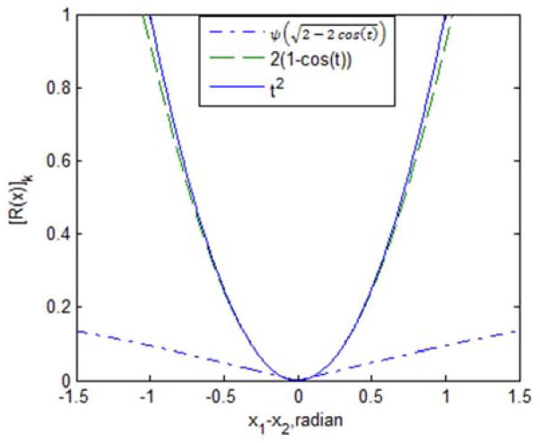
comparison of regularizer 1: t², regularizer 2: 2(1 − cos(t)), and regularizer 4: $\psi (\sqrt{2-2\mathit{cos}(t)})$.

C. Optimization Algorithms

Our goal is to estimate x and m from data y by minimizing the cost function:

$$(\widehat{\mathit{x}},\widehat{\mathit{m}})=\underset{\mathit{x},\mathit{m}\in {\mathbb{R}}^{N_p}}{\text{argmin}}{\mathrm{\Psi }}_l(\mathit{x},\mathit{m})$$ (18)

where l = 1, 2, 3 or 4, and N_p is the number of pixels in each image. We jointly estimate the phase and magnitude by alternately updating each of them in each iteration:

$${\mathit{x}}^{(n+1)}={\text{argmin}}_{\mathit{x}\in {\mathbb{R}}^{N_p}}{\mathrm{\Psi }}_l(\mathit{x},{\mathit{m}}^{(n)})$$ (19)

$${\mathit{m}}^{(n+1)}=\underset{\mathit{m}\in {\mathbb{R}}^{N_p}}{\text{argmin}}{\mathrm{\Psi }}_l({\mathit{x}}^{(n+1)},\mathit{m})$$ (20)

There are many optimization algorithms for CS, and we choose to use the iterative soft thresholding (IST) algorithm [10, Ch.12] to update m in (20). Specifically, we firstly design a separable quadratic surrogate function for the data fit term according to the optimization transfer principle [10, Ch.12], and then use the IST algorithm to minimize the surrogate function. The update formula was derived for real unknowns:

$${\mathit{m}}^{(n+1)}=U\ast \mathit{soft}\{U^{\prime }\ast {\mathit{m}}^{(n)}+\frac{1}{\check{c}}Re\{U^{\prime }{A}_x^{\prime }(\mathit{y}-A_x{\mathit{m}}^{(n)})\},\frac{{\beta }_2}{2\check{c}}\}$$ (21)

where $\mathit{soft}\{t;\alpha \}=\left(t-\alpha \ast \frac{t}{\mid t\mid }\right)\ast 1\{\mid t\mid >\alpha \},Re\{t\}$, Re{t} is the real part the complex number $t,A_x\triangleq A\ast \mathit{diag}\left\{e^{x_j^{(n+1)}}\right\}$, and č ≜ ρ(A′A), which is the spectral radius of A′A and e.g., č = N_p when we use Cartesian sampling.

It is more challenging to update x, because the cost function for x is nonlinear and non-convex. One way to approach this problem is to use optimization transfer as in [5]. We have investigated this approach for the cost function with regularizer 1 by using De Pierro’s trick [12] to design a quadratic surrogate function. However, it turned out to converge very slowly. Although this algorithm may work well for images that are sparse in the image domain, e.g., angiography images, we prefer to minimize the cost function in a more generally practical way. Therefore, we apply preconditioned conjugate gradient with backtracking line search (PCG-BLS) algorithm [10, Ch.11] to mitigate such problem. The updating formula is derived as follows (see appendix for details):

$${\mathit{x}}^{(n+1)}={\mathit{x}}^{(n)}+{\widehat{\alpha }}_n{\mathit{d}}^{(n)}$$ (22)

where d⁽ⁿ⁾ is the search direction derived by PCG algorithm [10, Ch.11], α̂_n is the step size α at the nth iteration which is chosen by Newton-Raphson algorithm with backtracking strategy to guarantee monotonicity [10, Ch.11]. The formula of the Newton-Raphson algorithm for updating the step size is:

$${\alpha }^{(k+1)}={\alpha }^{(k)}-\frac{{\stackrel{.}{\text{f}}}_{\text{n}}({\alpha }^{(\text{k})})}{{\ddot{\text{f}}}_{\text{n}}({\alpha }^{(\text{k})})}$$ (23)

where f_n(α) = Ψ_l(x⁽ⁿ⁾+ αd⁽ⁿ⁾, m⁽ⁿ⁾) These step size optimization formulas for the four regularizers are shown in the appendix respectively. Since this algorithm alone does not guarantee monotonicity, we need to use the backtracking strategy [13, p131] to ensure monotonic decrease of Ψ_l.

As one would expect, this nonlinear optimization algorithm has higher computational complexity than conventional CS optimization. For conventional CS by IST, the operations that dominate in each iteration are 2 A-operations, i.e., Fast Fourier transforms, and 2 U-operations, i.e., wavelet transforms. For the proposed method, updating m takes slightly shorter time than conventional CS, because although there are also 2 A-operations and 2 U-operations in each iteration, parts of them are real number operations instead of complex number operations in conventional CS optimization. However, the nonlinear optimization for x in the proposed method is much slower: in each iteration, there are 3Ns A-operations + 2Ns C-operations, i.e., taking finite difference transform, for computing the gradients, 3Ns*Na A-operations + 3 Ns*Na C-operations for the Newton-Raphson updating, and Ns*Na*Nb A-operations + Ns*Na*Nb C-operations for the backtracking part, where Ns is the number of sub-iterations in each iteration, Na is the number of iterations for the line search and Nb-1 is the number of backtracking steps. Empirically, we choose Ns = 2, and on average Na is 2.5 and Nb is about 1.1 on average; therefore, in each iteration, there are about 27 A-operations and 25 C-operations. A-operation is O(Nlog₂N), U-operation and C-operation are both O(N), where N represents N_d, N_p or K. Since we use first order finite difference and 3-level wavelet transform, C-operation is much faster than U-operation. Thus, the proposed method is roughly 10 times slower than conventional CS. However, we still achieve an acceptable computation time by the implementation shown in the appendix; for example, it takes about 55s to run the proposed method with 120 iterations for the 2D data in the in-vivo experiments of section III-C on a computer with Intel (R) Core (TM)2 Quad CPU Q9400 @ 2.66GHz, 4GB RAM and Matlab 7.8. For 3D data, a more efficient implementation in C++ may be necessary, but we believe that the computation time can be made acceptable.

As mentioned before, monotonically decreasing a non-convex cost function cannot guarantee finding a global minimizer for x for an arbitrary initial guess; therefore a good initial estimate for the phase image is important. In this study, since the cost function of conventional CS is convex, we set the initial guess for x and m by using the phase and magnitude of the result of conventional CS reconstruction method for complex voxels by IST (the cost function is like (4)). During this setup, we set the unknowns to be f = me^ix, and the initial guess of f is the inverse DFT of zero-padded k-space data; then we use a similar algorithm to (21) with some modifications:

$${\mathit{f}}^{(n+1)}=U\ast \mathit{soft}\left\{U^{\prime }\left({\mathit{f}}^{(n)}+\frac{1}{\check{c}}{A}^{\prime }(\mathit{y}-A{\mathit{f}}^{(n)})\right),\frac{{\beta }_2}{\check{c}}\right\}$$ (24)

Then we set x⁽⁰⁾ = ∠f⁽ⁿ⁾ and m⁽⁰⁾ = |f⁽ⁿ⁾| for n = 1 or 2 usually. Such initialization for phase and magnitude turns out to be very good for most cases except for regularizer 4 which has a narrower convex domain. To solve this problem, we take one more step to form the initial guess, which is to use regularizer 2 or 3 for a few iterations, because both of them have wider convex domains than regularizer 4. Then we believe we get the phase map closer to the desired phase map, which can help lead reconstructions using regularizer 4 to a desirable local minimum.

Like all the other regularized reconstruction methods, the regularization parameters should be carefully selected. For the parameter of the roughness penalty term, i.e., β₁, the value can be selected according to the desired spatial resolution of the phase image [1]. However, it is still an open problem for selecting parameters of the l₁ norm term. In this study, we choose the parameter β₂ empirically.

III. EXPERIMENTS

A. Experiments Setup

In our experiments, we compared the performance of the proposed methods with conventional phase-corrected CS that uses the IST algorithm (24) for optimization. All the data were sampled in the 2D Cartesian grid of k-space. The center of the k-space was fully sampled according to Nyquist sampling theorem, which preserves low frequency information and also allows for phase correction in conventional CS. The rest of k-space was randomly undersampled (as shown in Fig. 3). Three different image masks are used in the experiments: for reconstruction, we used a “loose” mask that was obtained from the inverse DFT of the raw undersampled data; in the results comparison, we use the true mask that is taken from the true image for a fair evaluation; for evaluation of the regions of interest (ROI), we use the ROI mask that is taken manually from the true phase image and only covers the ROIs. Regularization parameters were empirically chosen to be “the best” for each method, in terms of Normalized Root Mean Square Error (NRMSE) or Root Mean Square Error (RMSE) which were used for magnitude images and phase images respectively. NRMSE and RMSE are defined as below:

$$\mathit{NRMSE}=\frac{\left|\right|{\mathit{m}}_r-{\mathit{m}}_t\left|\right|}{\left|\right|{\mathit{m}}_t\left|\right|}$$ (25)

$$\mathit{RMSE}=\frac{\left|\right|{\mathit{x}}_r-{\mathit{x}}_t\left|\right|}{\sqrt{N_p}}$$ (26)

where m_r and m_t denote the reconstructed and true magnitude images respectively, x_r and x_t denote the reconstructed and true phase images respectively, and N_p is the number of pixels in each image. Moreover, we ran the algorithm until the cost function appeared to reach a minimum. In both methods, the sparse transform matrix (U) was set to be a 3-level Haar wavelet transform matrix which is unitary.

Fig. 3.

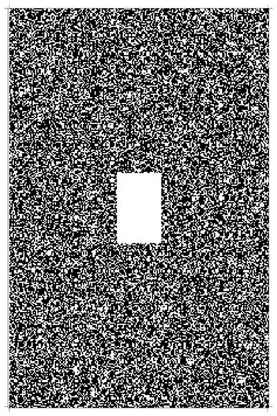
The sampling pattern in k-space

B. Experiments with simulated data

We simulated a thermometry scan using an abdomen T2 weighted magnitude image (upper left most in Fig. 4). We used the corresponding field map, scaled into the interval (−2π, 2π), as the background of the true phase map. The true complex image was cropped to be a 320*208 matrix (40cm *26cm FOV). To reduce the discretization effects that might happen in the synthesized data, we simulated the data from a higher resolution “true image”. Since there is not an analytical expression or a higher resolution version of this simulated object, we synthesized the higher resolution “true image” by linearly interpolating the original true image to be 960*624. In addition, we added four “Gaussian hot spots”, the peak values of which are from 3.5 to 4 radians, onto the interpolated background phase map to simulate thermal ablation (lower left most in Fig. 4). We chose this wide range of phase values to test performance of the proposed algorithm for wrapped phase maps. This “true complex image” is used as an approximation of the continuous phantom. Then we synthesized the fully sampled single-coil k-space data by taking DFT of the “true complex image”, and took the k-space data in a 320*208 matrix with sampling intervals corresponding to 40cm*26cm FOV. Then we added Gaussian distributed complex noise to mimic MRI scanner noise, and the noise level was fixed through all these simulation experiments such that the Signal-to-Noise-Ratio (SNR) was approximately 24 dB. The SNR is defined in k-space, which is

Fig. 4.

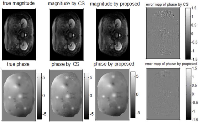
Top row: true magnitude, magnitude by CS, magnitude by the proposed method, phase error map by CS; bottom row: true phase, phase by CS, phase by the proposed method, phase error map by the proposed. (0.4 sampling rate, background is masked out, and the units of the phase are radians.)

$$\mathit{SNR}=20log\left(\frac{\left|\right|{\mathit{y}}_{\mathit{t}}\left|\right|}{\left|\right|{\mathit{y}}_{\mathit{t}}-\mathit{y}\left|\right|}\right)$$ (27)

where y_t denotes the noise-free k-space data, y denotes the noisy k-space data, and both are fully sampled in k-space. Afterwards, the final simulated data were formed by randomly sampling the Cartesian grid, with the center (3%) of the k-space fully sampled, as shown in Fig. 3.

In the experiments, the proposed method and conventional CS approach were tested at different sampling rates ranging from 20% to 60%. Since some referenceless PRF-shift temperature mapping methods [14] [15] have been proposed in literature, it is realistic to just reconstruct a certain frame without considering the reference frame in this simulation study. The reconstruction results are compared by visual inspection as well as NRMSE and RMSE of the reconstructed images with respect to the “low resolution true image”. This “low resolution true image” is obtained from the 320*208 fully sampled noiseless k-space data by an inverse DFT.

For conventional CS, we estimated the slow-varying reference phase map by taking the inverse DFT of the fully sampled k-space center. The proposed method used the regularizer 4 for the phase map, where we chose hyperbola function as the edge-preserving potential function, i.e., $\psi (t)={\delta }^2(\sqrt{1+{\mid t/\delta \mid }^2}-1)$ with δ = 0.0005 (radians) chosen empirically. The regularization parameters chosen for the simulation studies are shown in Table II.

Table II.

regularization parameters in the simulations

	0.2	0.3	0.4	0.5	0.6
β	1248	3744	2912	2912	4576
β1/106	10	8	5	7	7
β2	832	1248	1248	2080	2080

Fig. 5 compares NRMSE of magnitude maps with the true mask (called “entire magnitude” hereafter) and RMSE of phase maps with the true mask (called “entire phase” hereafter) at different sampling rates of conventional CS and the proposed method. We also compared the RMSE of the phase with the ROI masks, as shown in Fig. 5 (left), to evaluate the performance of the two methods for the regions around the hot spots, which are more important than other regions. The proposed method reduced NRMSE of the entire magnitude images by 10%~20%, while reduced the RMSE of the entire phase images by about 60%~70%; for the phase in the hot spots, the proposed method achieved about 50%~60% lower RMSE. Fig. 4 illustrates the results at 40% sampling rate; the regions outside the object have been masked out. Compared to conventional CS, the proposed method produces a much cleaner background phase map while preserving the hot spots information, especially for the hot spots in the low intensity regions where the important hot spots information is corrupted by noise in the results by conventional CS. However, the reduced NRMSE in the magnitude images is not very visible, which will be discussed in the next section.

Fig. 5.

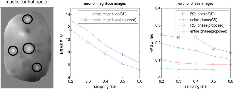
The regions masked for evaluating hot spots (left), NRMSE of the magnitude image (middle), RMSE of the entire phase image and RMSE of the phase masked for ROI, i.e., the hot spots, (right).

To demonstrate the importance of using regularizer 4, we replaced the regularizer 4 by regularizer 1–3 in the proposed method and reconstructed the data with 40% sampling rate. The regularization parameters are shown in Table III, and δ is set to 0.0005 radians for regularizer 3. Fig. 6 shows the phase maps and phase error maps of the reconstructed results. Regularizer 1 and regularizer 3 cannot handle the phase wrapped regions and tend to enhance the phase wrapping boundaries due to the smoothing within different convex domains; therefore, it is reasonable that regularizer 3 makes less “jumps” over the phase wrapping boundaries than regularizer 1 does. As expected, regularizer 2 tends to over-smooth the hot spots, especially the one pointed by the arrow; however, as shown in Fig. 1, regularizer 2 still has some edge-preserving effect, so the result by regularizer 2 was not far from the true phase; but it still not as good as the result by regularizer 4 (shown in Fig. 4). Table III also shows the RMSEs of ROI in the phase maps by regularizer 1–4. For initializing the proposed method, we believe that the results obtained by regularizer 2 or 3 tend to be in the convex domain that contains desired local minimum of the ultimate cost function with regularizer 4.

Table III.

regularization parameters in the simulations

	Reg. 1	Reg. 2	Reg. 3	Reg. 4
β1/104	1	1	800	500
β2	2912	2912	2912	1248
RMSE of ROI (radians)	0.930	0.087	0.282	0.081

Fig. 6.

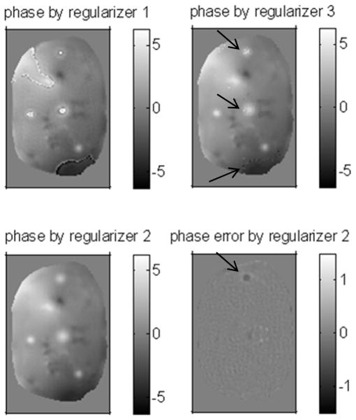
The reconstructed phase or phase error map by regularizer 1–3, the units are in radians

C. Experiments with In-vivo Data

We acquired in-vivo velocity mapping data around human abdominal aorta using a phase-contrast bSSFP sequence in 3T GE scanner (Signa Excite HD) with an 8-channel cardiac surface coil array. These multi-coil Cartesian sampled data contain 10 temporal frames as well as the reference frame (no velocity encoding). In each frame, the Cartesian grid is 160*160 which covers a FOV of 16cm*16cm. For demonstrating the 2D reconstruction algorithm for single coil, we used the reference frame and the 6th frame (capturing the peak velocity of the aorta) in coil 2 where the aorta signal is strong. Since the original data are fully sampled, we randomly undersampled them in the manner as in Fig. 3 to mimic the compressed sensing sampling; in particular, the sampling rate was chosen to be 1/3 of fully sampling, including 4% of fully sampled center.

Due to the reference frame, the reconstruction procedure was slightly different from the simulation experiment. Instead of reconstructing from one set of 2D data, we first reconstructed the reference frame by each method, and then we reconstructed the velocity encoded image with background phase removed by incorporating the reconstructed reference frame into the system matrix, which is a similar strategy to phase correction in CS as shown in (7). The cost functions of the two methods for the second step are shown below:

$$\mathrm{\Psi }({\mathit{f}}_1)={\left|\right|\mathit{y}-A(e^{i\mathit{P}}·\ast e^{{i\mathit{R}}_{\mathit{p}}}·\ast {\mathit{f}}_1)\left|\right|}^2+\beta R({\mathit{f}}_1)$$ (28)

$$\mathrm{\Psi }({\mathit{x}}_1,\mathit{m})={\left|\right|\mathit{y}-A(e^{{i\mathit{R}}_{\mathit{p}}}.\ast \mathit{m}.\ast e^{{i\mathit{x}}_1})\left|\right|}^2+{\beta }_1{R}_x({\mathit{x}}_1)+{\beta }_2{R}_m(\mathit{m})$$ (29)

where (28) and (29) are for CS and the proposed method respectively, R_p is the reference phase which contains no velocity information, f₁ should contain only velocity information in its phase, and x₁ should contain only velocity information. In (28), the CS method also has low frequency phase correction. In the proposed method, we used regularizer 2 to reconstruct the reference image, a smooth phase map, as it has no velocity encoding; we used the regularizer 4 to reconstruct the velocity map. Furthermore, we also investigated the performance of the proposed method with regularizer 1–3. The potential function for regularizer 4 (regularizer 3) was the hyperbola function with δ = 0.005 (radians). The regularization parameters for all the experiments are shown in Table IV.

Table IV.

regularization parameters in the in-vivo experiments

	CS	Reg. 4	Reg. 1	Reg. 2	Reg. 3
β1/103		60	5	5	50
β or β2	800	800	800	800	800

The results are shown in Fig. 7. In this experiment, since there is no “true” image for comparison, the reconstruction results from the fully sampled data by inverse DFT are shown in the first row of Fig. 7 for comparison; the second and the third row are the results by CS and the proposed method respectively. In the figure, the first, second and third column are the magnitude images, the reference phase maps and the velocity maps respectively. Similar to the simulation experiment, both of the methods (CS and the proposed) can reconstruct a comparably good magnitude image from undersampled data. In the second column of Fig. 7, the reference phase map produced by the proposed method is much smoother than that by conventional CS. In the last column, the proposed method gives us a velocity map that clearly shows a bifurcated aorta on top of a reasonably smooth background, which is much less noisy than the noisy velocity map produced by conventional CS.

Fig. 7.

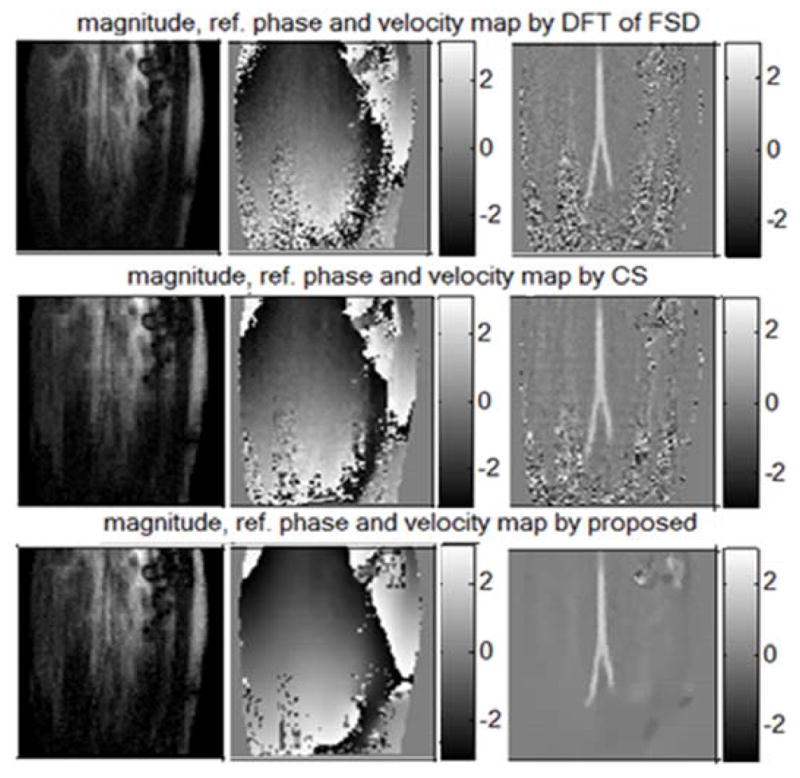
From the 1st row to the 3rd row: results by inverse DFT, conventional CS and the propose method; from the 1st column to the 3rd column: the magnitude, the reference phase and the velocity map. (The units of 2nd and 3rd columns are radians and cm/s respectively)

In the right upper corner of the velocity map by the proposed method (Fig. 7), there is an area that is not smooth; this is due to the inconsistency between the reference frame and the velocity encoded frame, which appears to be caused by the unreliable reference phase in that low intensity area.

Fig. 8 shows the phase maps reconstructed by the proposed method with regularizer 1, 2 and 3. Similar to the results in the simulation studies, while regularizer 2 smooths the background (except for the phase wraps), it also tends to over-smooth the arteries, which is undesirable. Since this particular problem has no phase wraps if initialized properly, the result by regularizer 1 just has some over-smoothed arteries and the one by regularizer 3 is as good as the one by regularizer 4 (shown in Fig. 7); both of them do not have phase wrapping problem. Then for this case, regularizer 3 provides better initialization than regularizer 2.

Fig. 8.

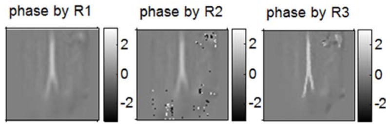
“R” denotes “regularizer”; left: phase map by the proposed method with R1; middle: phase map by the proposed method with R2; right: phase map by the proposed method with R3

IV. DISCUSSION

We have proposed two cost functions (13) & (15) and iterative algorithms (21)–(23) for reconstruction of magnitude and phase from undersampled k-space data. The key property of the proposed method is that one can adapt the regularizer for the magnitude and phase images individually.

The cost function is non-convex, so we cannot guarantee that the algorithm will converge to a global minimum. To mitigate this drawback, we introduced some suitable strategies for initialization. According to the simulation studies and real data experiments, it suffices to initialize by inverse DFT of zero-padded k-space and a few CS iterations for complex images when we apply regularizer 1, 2 or 3 appropriately. Since the cost function with regularizer 4 has a narrower convex domain, such two-step initialization does not always work; so a third step is added to the initialization as mentioned in the theory section. The logic behind these sequential initialization strategies is: optimizing the cost function with a wider convex domain is likely to “push” the initial guess towards the relatively narrower convex domain of the cost function that is optimized in the following step, when these two cost functions have similar optimization solutions. For initialization of the cost function with regularizer 4, the first step by inverse DFT sets the initial guess in the convex domain of the non-concave conventional CS cost function, then optimizing CS cost function pushes the initial guess to the convex domain (around a desired local minimum) of the proposed cost function with regularizer 2 or 3, and finally optimization in the third step make the initial guess reach the convex domain (around a desired local minimum) of the proposed cost function with regularizer 4. In a word, the initial guess is gradually “pushed” towards the convex domain of the final cost function by such sequential initialization steps. However, these strategies cannot theoretically guarantee finding a desirable minimum and are only successful empirically. Refining the initialization for this type of non-convex cost function is still an open problem for future research.

When using regularizer 4, we choose among various edge-preserving potential functions. We have investigated all the potential functions listed in [10, Ch.2] that have a bounded ω̇_ψ and most of them work well; finally we chose the hyperbola function because it has the widest convex domain and can match the quadratic function (t²) very well when neighboring pixels have similar phase values. The parameter δ determines the transition between smoothing and edge-preserving, hence it should be selected according to the features of the specific true phase map. In our experiments, we empirically discovered that the peaks of the hot spots or arteries tend to be over-smoothed if δ is selected according to t_edge, i.e., the amount of jumps that happen in the “edge” regions. Alternatively, we chose δ to be much smaller than t_edge, in which case the regularizer 2 or 4 is approximately a Total Variation (TV) regularizer [4], as the hyperbola potential function becomes approximately taking l₁ norm. Since TV still functions as edge-preserving regularization, it is still reasonable to use small δ for the proposed method. As long as δ is sufficiently small, we do not want it to be too small, because that will slower the convergence of the algorithm. Since the edges in the in-vivo data are sharper than the ones in the simulation data, δ in the in-vivo data was chosen to be larger than the one for the simulation data, but both of them are sufficiently smaller than t_edge. In a word, we empirically chose δ such that it is sufficiently small and also preserves an acceptable convergence rate.

The fully sampled k-space center is necessary for both conventional CS and the proposed method. For conventional CS, this part of the data is used to perform a rough phase-correction. In the proposed method, this low frequency part of the k-space contains most information of the phase map which has a smooth background. Empirically, 2~5% of the k-space center is sufficient to preserve the low frequency information of phase maps.

As can be seen in the simulation results, magnitude maps produced by the proposed method merely have a 10–20% lower NRMSE than the CS method in the simulation study and preserve a few more details if one carefully inspects, but this is not a significant improvement. Similar results were also observed in the in-vivo data experiments. In fact, this relatively small improvement is expected, because conventional phase-corrected CS has already removed most of the phase component of the true image before the CS reconstruction procedure. Therefore, the magnitude image in the proposed method is not significantly sparser than the phase corrected complex images in wavelet domain, which means the proposed method does not have much potential to significantly improve the magnitude image quality.

In the in-vivo experiment, although the phase map of conventional CS reconstruction looks closer to the fully sampled reconstruction, it does not indicate that it is closer to the true image; because the phase of the fully sampled reconstruction in the low intensity regions is dominated by noise. According to the physics, the true phase map should be smooth except for the distinct regions, e.g., arteries, so we believe that the smoothed background of the phase maps reconstructed by the proposed method are closer to the true phase map. Similarly, the reference frame of the velocity mapping reconstructed by the proposed method with regularizer 2 should be more accurate than the noisy map estimated by conventional CS, which is one of the reasons why the velocity map reconstructed by the proposed method is better.

Our method can potentially be used for field map estimation. In [1], the method is based on the reconstructed image, but it is ultimately better to estimate phase changes based on the raw k-space data, because the image itself may suffer from some undesirable artifacts. Our method not only estimates the phase based on the k-space data, but also could accelerate the acquisition by undersampling, which is useful for 3D and/or high resolution field map estimation.

In this paper, we only discussed the reconstruction problem for data from single coil acquisitions. However, all the proposed cost functions can also be easily generalized for parallel imaging, e.g. SENSE [11], to achieve an even lower sampling rate in k-space. Though we only studied 2D data, any higher dimensional data are applicable in the proposed method. The random sampling we used in the experiments simulates the random phase encode sampling in 3D data acquisition. Furthermore, this method is also applicable for non-Cartesian sampling by using non-uniform fast Fourier transform [16] as the system matrix.

The proposed method provides a more flexible and more controllable algorithm for phase map reconstruction than conventional phase corrected CS approach. The proposed method is flexible enough to allow customizing regularizers for phase component according to its own features, and regularizer 1–4 are concrete examples suitable for some applications; other sophisticated regularizers can be developed for other types of phase maps in this reconstruction framework. In addition, even though in some cases the results of phase corrected CS are acceptable, it is not as flexible for tuning the smoothness or resolution of the phase map as the proposed method. If one wants to increase the resolution of a non-smooth phase map when using phase corrected CS, another scan with different sampling rate may be required; in contrast, within a certain range, the proposed method can handle this by simply adjusting regularization parameters in reconstruction for the same data.

V. CONCLUSION

By using the CS regularization terms for magnitude, the proposed method allows for undersampling in data acquisitions. In the framework of separate regularization reconstruction, the proposed method achieves a substantial improvement, e.g., 50%–70%, in phase reconstruction and a minor improvement, e.g., 10%–20%, in magnitude reconstruction, compared to the phase corrected CS reconstruction. RMSE of ROI in phase maps were compared in the simulation studies to show that the proposed method can improve both ROI and background phase. Regularizer 1–4 were investigated for the simulated data and the in-vivo data, demonstrating that with initialization by using regularizer 2 or 3, the proposed method with regularizer 4 is able to handle phase wrapping and also reconstructs good phase maps and magnitude maps for applications like PRF-shift temperature mapping and phase contrast velocity mapping. The proposed method has more computational complexity, e.g., about ten times, than conventional CS, but we believe the computation speed can be made acceptable.

Table I.

summary of the four regularizers

Regularizer 1	R1(x) = ||Cx||2
Regularizer 2	R2(x) = ||Ceix||2
Regularizer 3	$R_3(\mathit{x})={\sum }_{k=1}^K\psi ({[C\mathit{x}]}_k)$
Regularizer 4	$R_4(x)={\sum }_{k=1}^K\psi (\mid {[{Ce}^{ix}]}_k\mid )$

Appendix

PCG-BLS for updating x:

1. The cost function for x:

   $$\mathrm{\Psi }(\mathit{x},{\mathit{m}}^{(n)})={\left|\right|\mathit{y}-{A\mathit{m}}^{(n)}{e}^{i\mathit{x}}\left|\right|}^2+{\beta }_1{R}_x(\mathit{x})+{\beta }_2{\left|\right|U^{\prime }{\mathit{m}}^{(n)}\left|\right|}_1$$ (30)

   where R_x(x) represents any possible regularizer for the phase map, including the 4 regularizers discussed in this paper.

2. The general formula for the Newton-Raphson algorithm in the line search for PCG:

   Let define a 1D cost function for the optimized step size α:

   $$f_n(\alpha )={\mathrm{\Psi }}_l({\mathit{x}}^{(n)}+\alpha {\mathit{d}}^{(n)},{\mathit{m}}^{(n)})$$ (31)
   where d⁽ⁿ⁾ is the search direction for x⁽ⁿ⁺¹⁾ by PCG algorithm. Using (8),

   $$f_n(\alpha )=L({\mathit{x}}^{(n)}+\alpha {\mathit{d}}^{(n)})+{\beta }_1{R}_l({\mathit{x}}^{(n)}+\alpha {\mathit{d}}^{(n)})$$ (32)

   where L(x) ≜ ||y − Am⁽ⁿ⁾e^ix||².

   Then we update x as the following:

   $${\mathit{x}}^{(n+1)}={\mathit{x}}^{(n)}+{\widehat{\alpha }}_n{\mathit{d}}^{(n)}$$ (33)
   where α̂_n denotes the optimized step size α and it is updated as follows:

   $$\therefore {\alpha }^{(k+1)}={\alpha }^{(k)}-\frac{{\stackrel{.}{\text{f}}}_{\text{n}}({\alpha }^{(\text{k})})}{{\ddot{\text{f}}}_{\text{n}}({\alpha }^{(\text{k})})}$$ (34)
   where

   $${\stackrel{.}{\text{f}}}_{\text{n}}(\alpha )={{\mathit{d}}^{(n)}}^{\prime }[\mathbf{\nabla }L({\mathit{x}}^{(n)}+\alpha {\mathit{d}}^{(n)})+{\beta }_1\mathbf{\nabla }{R}_l({\mathit{x}}^{(n)}+\alpha {\mathit{d}}^{(n)})]$$ (35)

   $${\ddot{\text{f}}}_{\text{n}}(\alpha )={{\mathit{d}}^{(n)}}^{\prime }[{\mathbf{\nabla }}^{2}L({\mathit{x}}^{(n)}+\alpha {\mathit{d}}^{(n)})+{\beta }_1{\mathbf{\nabla }}^2{R}_l({\mathit{x}}^{(n)}+\alpha {\mathit{d}}^{(n)})]{\mathit{d}}^{(n)}$$ (36)

3. Gradients and Hessian matrices (real unknowns):

   1. The data fit term L(x):

      $$\mathbf{\nabla }L(\mathit{x})=2Re\{\mathit{diag}\{{ie}^{-i\mathit{x}}\}[A_m^{\prime }(\mathit{y}-A_m{e}^{i\mathit{x}})]\}=2Re\{{\mathit{g}}_{\mathbf{1}}(\mathit{x})\}$$ (37)

      $${\mathbf{\nabla }}^{2}L(\mathit{x})=2Re\left\{\mathit{diag}\{e^{-i\mathit{x}}.\ast A_m^{\prime }(\mathit{y}-A_m{e}^{i\mathit{x}})\}+\mathit{diag}\{e^{-i\mathit{x}}\}{A}_m^{\prime }{A}_m\mathit{diag}\{e^{i\mathit{x}}\}\right\}$$ (38)
      where A_m ≜ A * diag{m⁽ⁿ⁾}, “.*” means entry-by-entry multiplication, ${\mathit{g}}_{\mathbf{1}}(\mathit{x})\triangleq \mathit{diag}\{{ie}^{-i\mathit{x}}\}[A_m^{\prime }(\mathit{y}-A_m{e}^{i\mathit{x}})]$. Note that since ∇² L(x) is only used in (36), the equation (38), which is very expensive, does not need to be computed explicitly. Combining (36)–(38) yields an efficient expression for f̈_n(α):

      $${\ddot{\text{f}}}_{\text{n}}(\alpha )=2\left(Re\left\{{{\mathit{d}}^{(n)}}^{\prime }[(-{\mathit{ig}}_{\mathbf{1}}(\mathit{x}\_\mathit{d})).\ast {\mathit{d}}^{(n)}]\right\}+{{\mathit{b}}_{\mathbf{1}}}^{\prime }{\mathit{b}}_{\mathbf{1}}\right)+{\ddot{\text{f}}}_{\text{R},\text{n}}(\alpha )$$ (39)

      where x_d ≜ x⁽ⁿ⁾ + αd⁽ⁿ⁾, b₁ ≜ A_mdiag{e^ix_d}d⁽ⁿ⁾, and f̈_R,n(α) ≜ β₁d ^(n)′∇²R_x(x_d)d ⁽ⁿ⁾.

   2. The regularizer R₁(x):

      1. Regularizer 1:

         $$R_1(\mathit{x})={\left|\right|C\mathit{x}\left|\right|}^2$$ (40)

         $$\mathbf{\nabla }{R}_1(\mathit{x})=2C^{\prime }C\mathit{x}$$ (41)

         $${\mathbf{\nabla }}^2{R}_1(\mathit{x})=2C^{\prime }C$$ (42)

         In (39), f̈_R,n(α) can be simplified as: f̈_R,n(α) = 2β₁||Cd⁽ⁿ⁾||².

      2. Regularizer 2:

         $$R_2(\mathit{x})={\left|\right|{Ce}^{i\mathit{x}}\left|\right|}^2$$ (43)

         $$\begin{array}{l}\mathbf{\nabla }{R}_2(\mathit{x})=-2Re\{{ie}^{-i\mathit{x}}.\ast [C^{\prime }{Ce}^{i\mathit{x}}]\}\\ =-2Re\{{\mathit{g}}_{\mathbf{2}}(\mathit{x})\}\end{array}$$ (44)

         $${\mathbf{\nabla }}^2{R}_2(\mathit{x})=2Re\{\mathit{diag}(e^{-i\mathit{x}})C^{\prime }\mathit{Cdiag}\{e^{i\mathit{x}}\}-\mathit{diag}\{e^{-i\mathit{x}}.\ast (C^{\prime }{Ce}^{i\mathit{x}})\}\}$$ (45)

         where g₂(x) ≜ ie^−ix.* [C′Ce^ix].

         In (39), f̈_R,n(α) = 2β₁(Re{d^(n)′[(−ig₂(x_d)).* d⁽ⁿ⁾]} + b₂′b₂), where b₂ ≜ Cdiag{e^ix_d}d ⁽ⁿ⁾.

      3. Regularizer 3:

         $$R_3(\mathit{x})=\sum _{k=1}^K{\psi }_k({[C\mathit{x}]}_k)$$ (46)

         $$\mathbf{\nabla }{R}_3(\mathit{x})=C^{\prime }\mathit{diag}\{{\omega }_{\psi }(C\mathit{x})\}C\mathit{x}$$ (47)

         $${\mathbf{\nabla }}^2{R}_3(\mathit{x})=C^{\prime }\mathit{diag}\{{\ddot{\psi }}_k(C\mathit{x})\}C$$ (48)

         In (39), f̈_R,n(α) = 2β₁p′ diag{ψ̈_k(Cx_d)}p, where p ≜ Cd⁽ⁿ⁾.

      4. Regularizer 4:

         $$R_4(\mathit{x})=\sum _{k=1}^K{\psi }_k(\mid {[{Ce}^{i\mathit{x}}]}_k\mid )$$ (49)

         $$\mathbf{\nabla }{R}_4(\mathit{x})=-Re\{{ie}^{-i\mathit{x}}.\ast [C^{\prime }\mathit{diag}\{{\omega }_{\psi }(\mid {Ce}^{ix}\mid )\}{Ce}^{i\mathit{x}}]\}$$ (50)

         $$\begin{array}{l}{\mathbf{\nabla }}^2{R}_4(\mathit{x})=-Re\left\{\mathit{diag}\{e^{-i\mathit{x}}.\ast [C^{\prime }\mathit{diag}\{{\omega }_{\psi }(\mid {Ce}^{ix}\mid )\}{Ce}^{i\mathit{x}}]\}\right\}\\ +Re\left\{\mathit{diag}\{e^{i\mathit{x}}\}{C}^{\prime }\mathit{diag}\{{\omega }_{\psi }(\mid {Ce}^{ix}\mid )\}\mathit{Cdiag}\{e^{i\mathit{x}}\}\right\}+\\ Re\{i\ast \mathit{diag}\{e^{-i\mathit{x}}\}{C}^{\prime }\mathit{diag}\{{\stackrel{.}{\omega }}_{\psi }(\mid {Ce}^{ix}\mid ).\ast ({Ce}^{ix})./\mid {Ce}^{ix}\mid \}\}\ast Re\left\{i\ast \mathit{diag}\{{Ce}^{i\mathit{x}}\}\mathit{Cdiag}\{e^{-i\mathit{x}}\}\right\}\end{array}$$ (51)

         where g₃(x) ≜ ie^−ix.* [C′diag{ω_ψ(|Ce^ix|)}h(x)], and h(x) ≜ Ce^ix.

         In (39), ${\ddot{\text{f}}}_{\text{R},\text{n}}(\alpha )=2{\beta }_1\left(Re\{{{\mathit{d}}^{(n)}}^{\prime }\left[(-{\mathit{ig}}_{\mathbf{3}}(\mathit{x}\_\mathit{d})).\ast {\mathit{d}}^{(n)}\right]\}+{\mathit{b}}_2^{\prime }\mathit{diag}\{{\omega }_{\psi }(\mid \mathit{h}(\mathit{x}\_\mathit{d})\mid )\}{\mathit{b}}_2+{\mathit{b}}_3{\mathit{b}}_4\right)$, where b₃ ≜ Re{i*b₂′ diag{ω̇_ψ(|h(x_d)|).* (h(x_d))./|h(x_d)|}}, x̄ denotes the conjugate of x, and ${\mathit{b}}_{\mathbf{4}}\triangleq Re\{i\ast \mathit{diag}\{\mathit{h}(\mathit{x}\_\mathit{d})\}\overline{{\mathit{b}}_{\mathbf{2}}}\}$.

References

- 1.Funai AK, Fessler JA, Yeo D, Olafsson VT, Noll DC. Regularized Field Map Estimation in MRI. IEEE Trans on Medical Imaging. 2008 Oct;27(10):1484–1494. doi: 10.1109/TMI.2008.923956. [DOI] [PMC free article] [PubMed] [Google Scholar]
- 2.Poorter JD, Wagter CD, Deene YD, Thomsen C, Stahlberg F, Achten E. NoninvasiveMRI thermometry with the proton resonance frequency (PRF) method: in vivo results in human muscle. Magnetic Resonance in Medicine. 1995;33(1):74–81. doi: 10.1002/mrm.1910330111. [DOI] [PubMed] [Google Scholar]
- 3.Nielsen J-F, Nayak KS. Referenceless Phase Velocity Mapping Using Balanced SSFP. Magnetic Resonance in Medicine. 2009 May;61(5):1096–1102. doi: 10.1002/mrm.21884. [DOI] [PubMed] [Google Scholar]
- 4.Rudin LI, Osher S, Fatemi E. Nonlinear total variation based noise removal algorithm. Physica D. 1992 Nov;60(1–4):259–68. [Google Scholar]
- 5.Fessler JA, Noll DC. Iterative image reconstruction in MRI with separate magnitude and phase regularization. Proc IEEE Intl Symp Biomed Imag. 2004:209–12. [Google Scholar]
- 6.Lustig M, Donoho D, Pauly JM. Sparse MRI: The Application of Compressed Sensing for Rapid MR Imaging. Magnetic Resonance in Medicine. 2007;58:1182–1195. doi: 10.1002/mrm.21391. [DOI] [PubMed] [Google Scholar]
- 7.Bydder M, Robson MD. Partial fourier partially parallel imaging. Magn Reson Med. 2005 Jun;53(6):1393–40. doi: 10.1002/mrm.20492. [DOI] [PubMed] [Google Scholar]
- 8.Noll C, Nishimura DG, Macovski A. Homodyne detection in magnetic resonance imaging. IEEE Trans Med Imag. 1991;10:154–163. doi: 10.1109/42.79473. [DOI] [PubMed] [Google Scholar]
- 9.Zibetti MVW, De Pierro AR. Separate magnitude and phase regularization in MRI with incomplete data: Preliminary results. IEEE Int Symp Biomed Imag. 2010 [Google Scholar]
- 10.Fessler JA. Image Reconstruction: Algorithms and Analysis. in preparation. [Google Scholar]
- 11.Pruessmann KP, Weiger M, Scheidegger MB, Boesiger P. SENSE: Sensitivity Encoding for Fast MRI. Magnetic Resonance in Medicine. 1999;42:952–962. [PubMed] [Google Scholar]
- 12.De Pierro AR. A modified expectation maximization algorithm for penalized likelihood estimation in emission tomography. IEEE Trans Med Imag. 1995 Mar;14(1):132–7. doi: 10.1109/42.370409. [DOI] [PubMed] [Google Scholar]
- 13.Lange K. Numerical analysis for statisticians. Springer-Verlag; New York: 1999. p. 131. [Google Scholar]
- 14.Rieke, Vigen K, Sommer G, Daniel BL, Pauly JM, Butts K. Referenceless PRF shift thermometry. Magnetic Resonance in Medicine. 2004;51(6):1223–1231. doi: 10.1002/mrm.20090. [DOI] [PubMed] [Google Scholar]
- 15.Grissom W, Pauly KB, Lustig M, Rieke V, Pauly J, McDannold N. Regularized referenceless temperature estimation in PRF-shift MR thermometry. IEEE Int Symp Biomed Imag. 2009 [Google Scholar]
- 16.Fessler JA, Sutton BP. Nonuniform fast fourier transforms using min-max interpolation. IEEE Trans Signal Process. 2003 Feb;51(2):560–574. [Google Scholar]
- 17.Cetin M, Karl WC. Feature-enhanced synthetic aperture radar image formation based on nonquadratic regularization. IEEE Tr Im Proc. 2001 Apr;10(4):623–31. doi: 10.1109/83.913596. [DOI] [PubMed] [Google Scholar]