Statistically significant contrasts between EMG waveforms revealed using wavelet-based functional ANOVA

Abstract

We developed wavelet-based functional ANOVA (wfANOVA) as a novel approach for comparing neurophysiological signals that are functions of time. Temporal resolution is often sacrificed by analyzing such data in large time bins, increasing statistical power by reducing the number of comparisons. We performed ANOVA in the wavelet domain because differences between curves tend to be represented by a few temporally localized wavelets, which we transformed back to the time domain for visualization. We compared wfANOVA and ANOVA performed in the time domain (tANOVA) on both experimental electromyographic (EMG) signals from responses to perturbation during standing balance across changes in peak perturbation acceleration (3 levels) and velocity (4 levels) and on simulated data with known contrasts. In experimental EMG data, wfANOVA revealed the continuous shape and magnitude of significant differences over time without a priori selection of time bins. However, tANOVA revealed only the largest differences at discontinuous time points, resulting in features with later onsets and shorter durations than those identified using wfANOVA (P < 0.02). Furthermore, wfANOVA required significantly fewer (∼¼×; P < 0.015) significant F tests than tANOVA, resulting in post hoc tests with increased power. In simulated EMG data, wfANOVA identified known contrast curves with a high level of precision (r² = 0.94 ± 0.08) and performed better than tANOVA across noise levels (P < <0.01). Therefore, wfANOVA may be useful for revealing differences in the shape and magnitude of neurophysiological signals (e.g., EMG, firing rates) across multiple conditions with both high temporal resolution and high statistical power.

we often want to compare the shapes of waveforms that are functions of time, but traditional statistical methods cannot reveal differences between curves without sacrificing temporal resolution or power. Certain features of the waveforms that are clearly identifiable based on visual inspection may not be revealed by traditional statistical tests such as t-tests or ANOVA applied across time points due to the large number of comparisons (Fig. 1A; Abramovich et al. 2004; Fan and Lin 1998). For example, many studies present clear differences in mean waveforms across conditions in electromyograms (EMGs; Hiebert et al. 1994), H-reflex responses (Frigon 2004), kinematics (Ivanenko et al. 2005), and neural firing rates (Mushiake et al. 1991), but statistical tests are often not performed or reported due to low power. A common approach to overcome this problem is to apply statistical analyses to mean values over a time bin of interest (Frigon 2004; Welch and Ting 2009). However, this approach sacrifices the temporal resolution of the interesting feature by approximating it as a single data point. To address this undesirable trade-off between temporal resolution and statistical power, we propose performing statistical inference outside of the time domain.

Fig. 1.

Schematic illustrating ANOVA applied to waveforms in the time domain and in the wavelet domain. A: waveform comparison in the time domain (tANOVA). A₁: in highly variable waveform data such as electromyograms (EMGs), many noisy individual trials [y(t); gray] can be averaged into mean waveforms [μ(t); black] to estimate unknown underlying signals (green) in a given experimental condition (condition 2, above, or condition 1, below). A₂: ANOVA applied to individual time points identifies significant differences between experimental conditions only at discontinuous time points [μ₂(t) vs. μ₁(t); yellow] due to low power. B: waveform comparison in the wavelet domain (wfANOVA). B₁: in wfANOVA, noisy individual trials [y(t); gray lines, left] are transformed into the wavelet domain [Y(w); gray points, right] before statistical analysis. B₂: because of the compression properties of the wavelet transform, ANOVA identifies differences between experimental conditions in only a few significant wavelet coefficients that represent localized spatiotemporal features [M₂(t) vs. M₁(t); blue points, right] and that can then be transformed back into the time domain for visualization as continuous contrast curves [μ₂(t) vs. μ₁(t); red line, left].

The wavelet transform is a versatile tool for the analysis of waveforms with time-varying frequency content because it reveals not only the different frequency components of the waveform, but also the temporal structure of those components. Because of its power to describe signals containing events throughout the range of time-frequency localization, the wavelet transform has been used in many biomedical applications, including analysis of electroencephalogram and electrocardiogram signals and processing for positron emission tomography and MRI (see Unser and Aldroubi 1996 for a review). Like the Fourier transform, the wavelet transform decomposes the signal of interest into orthogonal basis functions with different frequency characteristics that additively represent the original signal. In contrast to the Fourier transform, the basis functions used in the wavelet transform are temporally localized. This property allows the representation of both frequency and temporal information within the transformed signal and provides a particularly rich description of biomedical signals, which often have nonstationary frequency composition and burstlike temporal structure (Cohen and Kovacevic 1996).

Previously, the wavelet transform has been used to identify features of EMG signals, but it has not been used for statistical comparison of EMG waveform across conditions (Cohen and Kovacevic 1996; Unser and Aldroubi 1996). For example, the wavelet transform has been used to quantify automatically the timing of bursts within EMG signals in a manner similar to template matching (Flanders 2002). Wavelet packets have also been used to quantify the temporal location and width of unit bursts in EMG signals (Hart and Giszter 2004) as well as for extraction and classification of motor unit action potentials from EMG records (Fang et al. 1999; Ostlund et al. 2006; Ren et al. 2006). Wavelet analyses have also been used to estimate latent information within EMG signals. For example, time-dependent power spectra (Huber et al. 2011; von Tscharner 2000; Wakeling and Horn 2009) as well as changes in these spectra, for example, with fatigue (Kumar et al. 2003), have been estimated to offer information about underlying muscle fiber conduction velocity (Stulen and De Luca 1981). However, to our knowledge, the wavelet transform has not been previously applied in the context of hypothesis testing for comparison of waveform shapes (Unser and Aldroubi 1996).

Here, we leveraged the beneficial properties of the wavelet transform to develop a generalized technique called wavelet-based functional ANOVA (wfANOVA) to compare statistically the shapes of waveforms that are functions of time without sacrificing temporal resolution or statistical power. Our method is related to functional data analysis (Ramsay and Silverman 2005) because each wavelet is a function of time rather than a single time point. When expressed in the wavelet domain, temporally localized waveform features tend to be well-represented by a few wavelets rather than by many correlated time samples (Fig. 1B) or by many independent sinusoids as in Fourier analysis. Therefore, applying statistical tests to wavelet coefficients reduces the number of statistical tests required while retaining statistical power (Angelini and Vidakovic 2003). In contrast to many wavelet-domain techniques that have been applied to EMG data, wfANOVA does not use information about the wavelet coefficients themselves to suppose possible physiological mechanisms that may have generated the EMG signals (e.g., subpopulations of motor units or muscle fiber types). Rather, wavelets are used only as basis functions that correspond to these localized time differences that are easily identifiable by eye. The unique and generalizable attribute of wfANOVA is the reconstruction of the wavelets into the time domain after performing functional analyses to allow the visualization of the effects of experimental manipulation as contrast curves in the time domain (Fig. 1B) rather than reporting these effects in the wavelet domain.

As proof of principle, we applied wfANOVA to previously published EMG data to demonstrate its ability as a general method for determining differences in the time courses of waveforms. We first compared the ability of wfANOVA and time-point ANOVA (tANOVA) to identify contrast curves in previously published EMG waveforms in response to perturbations during standing balance (Welch and Ting 2009) without picking time windows a priori. Previously, ANOVA was performed on mean values of EMG calculated during fixed time bins, demonstrating that peak perturbation acceleration alters the magnitude of early periods of EMG, whereas peak perturbation velocity affects later periods (Welch and Ting 2009; Fig. 2). Here, we perform a reanalysis of these data to test whether the effects of perturbation peak acceleration and peak velocity can be visualized as continuous contrast curves without relying on time windows chosen by the experimenter. Finally, we compared the ability of wfANOVA and tANOVA to identify known contrast curves in simulated EMG data with noise characteristics similar to those of recorded EMG data but with known temporal structure.

Fig. 2.

Effects of varying peak acceleration and peak velocity of perturbations on different periods of the EMG response. A: forward translation perturbations of the support surface elicit EMG activity in ankle dorsiflexor tibialis anterior (TA). B: examples of platform kinematics and TA EMG during perturbations with constant peak velocity level (30 cm/s) but peak acceleration level varying from low (0.1 g; black) to high (0.4 g; light gray). Vertical lines indicate the time windows previously used for the initial burst (IB) and plateau region (PR) time periods of muscle activity (Welch and Ting 2009). Regression analyses demonstrate significant scaling of EMG magnitude with perturbation characteristics during the IB period but not during the PR period. pos, Position; vel, velocity; accel, acceleration. *P < 0.05. C: examples of platform kinematics and TA EMG during perturbations with constant peak acceleration level (0.2 g) but peak velocity level varying from low (25 cm/s; black) to high (40 cm/s; light gray). Regression analyses demonstrate significant scaling of EMG with perturbation characteristics during the PR period but not during the IB period. Adapted with permission from Welch and Ting (2009).

METHODS

EMG data.

The experimental protocol was approved by the Institutional Review Boards of Emory University and Georgia Institute of Technology. We applied wfANOVA and tANOVA to previously published EMG waveforms recorded during postural perturbations elicited by translating the support surface forward or backward in the horizontal plane. Detailed experimental methods are presented in an earlier paper (Welch and Ting 2009). Briefly, 7 healthy subjects [2 female, 5 male, mean age 19.4 ± 1.4 yr (mean ± SD)] stood on a moveable platform that translated in the horizontal plane. Subjects withstood translation perturbations of the support surface that were designed so that platform peak acceleration and peak velocity could be varied independently. Perturbations were delivered with peak velocities of 25, 30, 35, and 40 cm/s and peak accelerations of 0.2, 0.3, and 0.4 g. Although additional peak acceleration levels were administered to subjects, only the acceleration levels for which all levels of velocity could be achieved with the experimental apparatus were considered for further analysis in a balanced ANOVA design. Conditions were randomized, and each subject was nominally exposed to each of the conditions 5 times, although in some cases trials were repeated or sessions ended early due to fatigue. We used all available trials for each of the 7 subjects, resulting in 33–38 trials in each of the 12 conditions (Table 1). We were particularly interested in the ability of wfANOVA and tANOVA to identify variation in EMG waveforms with perturbation characteristics within two 150-ms time bins referred to as the initial burst (IB) and plateau region (PR), respectively, beginning 100 ms after perturbation onset (Fig. 2).

Table 1.

Total number of replicates across subjects for each condition

		Acceleration Factor Level	1	2	3
Velocity Factor Level	Peak Velocity	Peak Acceleration	0.2 g	0.3 g	0.4 g	Total
1	25 cm/s		37 F, 36 B	37, 36	37, 37	111, 109
2	30 cm/s		37, 37	37, 36	37, 36	111, 109
3	35 cm/s		37, 37	38, 37	34, 38	109, 112
4	40 cm/s		38, 33	33, 37	37, 37	108, 107
		Total	149, 143	145, 146	145, 148	439, 437

F, number of forward perturbations for which tibialis anterior (TA) is the agonist; B, number of backward perturbations for which medial gastrocnemius (MG) is the agonist.

EMG was collected during each trial, processed, and registered to the onset of perturbation acceleration. We examined the activity of ankle dorsiflexor tibialis anterior (TA) during forward perturbations and ankle plantarflexor medial gastrocnemius (MG) during backward perturbations. Raw EMG signals were collected at 1,080 Hz, high-pass filtered at 35 Hz (3rd-order 0-lag Butterworth filter), demeaned, rectified, and low-pass filtered at 40 Hz (1st-order 0-lag Butterworth filter). EMG signals were resampled at 360 Hz, registered to platform onset to within 1 sample (<1 ms), and truncated to be 512 samples long (1.42 s), including 10 samples (0.03 s) before platform onset. EMG signals were normalized to the unit interval.

Mean difference curves.

Differences in average EMG waveform shape across levels of peak perturbation velocity and peak perturbation acceleration were visualized as mean difference curves. Grand mean time courses of EMG activity for each muscle and level of perturbation acceleration and velocity were calculated. Mean difference curves across perturbation levels were calculated by subtracting the grand mean time course from the lowest level of perturbation acceleration or velocity from each higher level. Mean difference curves represent the mean effect of increases in perturbation level but provide no information about whether any part of the curve corresponds to statistically significant effects.

Wavelet decomposition and structure of wavelet-transformed signals.

The structure of the discrete wavelet transform can be understood as generally analogous to that of the more familiar discrete Fourier transform in that both are linear transformations. Similar to the discrete Fourier transform, the discrete wavelet transform results in a number of wavelet coefficients equal to the number of time samples of the transformed signal (Fig. 3, A and B), provided the length of the signal is a power of two. Signals can be padded with zeroes or symmetrically extended to appropriate length. This one-to-one correspondence is advantageous for both transforms because it provides a reversible linear transformation from the original signal to the wavelet (or Fourier) domain and back. Wavelet basis functions are typically orthogonal, as are the sinusoidal elements that form the basis in the Fourier domain. This orthogonality is important for statistical inference, as multivariate procedures such as multivariate ANOVA (MANOVA) break down when high correlations are observed between variables, as in time series data. Because observations in the wavelet domain or Fourier domains are nearly uncorrelated (Angelini and Vidakovic 2003; Fan and Lin 1998; Vidakovic 2001), these effects are minimized.

Fig. 3.

Schematic comparison of discrete Fourier transform and discrete wavelet transform. A: in the discrete Fourier transform, 512 time samples are transformed into an identical number of unique coefficients in the frequency domain. B: in the discrete wavelet transform, the time signal is transformed to the wavelet domain through a recursive filtering and downsampling process, resulting in a blocked wavelet coefficient structure that is ordered in time as well as in frequency. The 1st block of “approximation” coefficients (a4) comprises a low-pass filtered, downsampled representation of the original signal. The remaining blocks of “detail” coefficients (d4–d1) represent successively higher frequency information that is absent from the approximation block. C: sinusoidal basis function for the DFT are infinite in time, whereas wavelet basis functions (D) are time-limited and temporally localized functions.

However, whereas the sinusoids that form the basis in the Fourier domain are infinite in time (Fig. 3C), wavelets are temporally localized functions that are nonzero only in small regions (Fig. 3D). Whereas Fourier transforms depend heavily on cancellation (Strang 1989), resulting in a large number of frequencies to reconstruct a square-wave, for example (Fig. 3C), many wavelet coefficients in the transformed data may be of small or zero magnitude (Fig. 3D). Therefore, signals can be compressed into fewer wavelet coefficients than original time samples by quantizing or eliminating small-magnitude coefficients. This enables the use of the wavelet transform as part of a data compression scheme (Unser and Aldroubi 1996).

In contrast to the discrete Fourier transform, in which the transformed coefficients are arranged in order of increasing frequency (Fig. 3A), the coefficients of the discrete wavelet transform are arranged in a blocked structure that is ordered in time as well as in frequency (Fig. 3B). This blocked structure results from the recursive filtering and downsampling process used to perform the discrete wavelet transform. The first block of coefficients, referred to as the “approximation” coefficients, comprise a low-pass filtered, downsampled representation of the original signal produced by convolving the signal with a low-pass filter (based on the approximation or “father” wavelet) and downsampling the filtered signal by a factor of two (Cohen and Kovacevic 1996). The approximation coefficients are arranged in order of increasing time, roughly representing the magnitude of the signal at that time point, which corresponds to the peak of the wavelet function for the third-order coiflets used here. The remaining blocks of coefficients, referred to as “detail” coefficients, represent successively higher frequency information that is absent from the approximation and are produced by convolving the signal with a high-pass filter based on the detail or “mother” wavelet. The coefficients within each detail block are also arranged in order of increasing time, although the length of the detail blocks increases with the frequency content. For the length 512 signals and level 4 wavelet decomposition used here, the approximation coefficients (level a4) are arranged in a block of length 32, followed by blocks of detail coefficients of length 32 (level d4), 64 (d3), 128 (d2), and 256 (d1) with progressively higher frequency content (Fig. 3B). To produce a multilevel wavelet decomposition, the signal is 1st divided into approximation and detail coefficients, and approximation coefficients are recursively divided into higher-level approximation and detail coefficients. The maximum number of recursions during the transform depends on both the length of the input signal and the particular wavelet chosen.

wfANOVA.

Individual EMG waveforms were transformed to the wavelet domain using the MATLAB wavelet toolbox (http://www.mathworks.com; The MathWorks) and analyzed with three-factor ANOVA (velocity × acceleration × subject). EMG signals were transformed using third-order coiflets (decomposition level 4; wavedec.m) with periodic extension. Coiflets were selected because they are symmetrical and therefore do not introduce phase distortions in the locations of the transformed signals. We assumed a fixed-effects three-factor ANOVA model (Sokol and Rohlf 1981) where each wavelet coefficient was comprised as:

$$Y_{ijkn}\left(\text{w}\right)=M\left(\text{w}\right)+A_i\left(\text{w}\right)+B_j\left(\text{w}\right)+C_k\left(\text{w}\right)+E_{ijkn}\left(\text{w}\right)$$ (1)

where M(w) designates the wavelet coefficients of the grand mean, A_i(w) designates the effects of the ith peak platform velocity level (among 25, 30, 35, and 40 cm/s), B_j(w) designates the effects of the jth peak platform acceleration level (among 0.2, 0.3, and 0.4 g), C_k(w) designates the effects of the kth subject (among 1–7), and E_ijkn(w) designates Gaussian random process noise on the nth replicate of that combination of other factors. Wavelet coefficients corresponding to significant initial F tests (anovan.m) at significance level α = 0.05 were then evaluated for significant contrast across velocity or acceleration levels with separate post hoc Scheffé tests to test the following null hypotheses:

$$H_{0A}:A_1=A_2=A_3=A_4$$ (2)

$$H_{0B}:B_1=B_2=B_3$$ (3)

After initial ANOVA, post hoc tests (multcompare.m) were performed for each of the velocity and acceleration factors at significance levels Bonferroni-corrected by the number of significant corresponding initial F tests. Contrasts in wavelet magnitude were calculated with respect to the lowest velocity and acceleration conditions. Statistically significant contrasts in wavelet coefficient magnitude were then assembled into wavelet-domain contrast curves and transformed back to the time domain. All coefficients of wavelet-domain contrast curves were initially zero; wavelet coefficients corresponding to significant contrasts were set to the estimate of the contrast. Wavelet-domain contrast curves were then transformed back to the time domain for visualization (waverec.m).

tANOVA.

tANOVA was performed identically to wfANOVA with the exception that it was performed entirely in the time domain. Similar to wfANOVA, three-way ANOVA (velocity × acceleration × subject) was performed at each time point at significance level α = 0.05. We assumed a fixed-effects three-factor ANOVA model where each time sample was comprised as

$$y_{ijkn}\left(t\right)=\mu \left(t\right)+{\alpha }_i\left(t\right)+{\beta }_j\left(t\right)+{\gamma }_k\left(t\right)+{\epsilon }_{ijkn}\left(t\right)$$ (4)

where μ(t) designates the grand mean, α_i(t) designates the effects of peak platform velocity level i, β_j(t) designates the effects of peak platform acceleration j, γ_k(t) designates the effects of subject k, and ϵ_ijkn(t) designates Gaussian random process noise on the nth replicate of that combination of other factors. Time points corresponding to significant initial F tests were then evaluated for significant contrast across velocity or acceleration levels with separate post hoc Scheffé tests to test the following null hypotheses:

$$H_{0\alpha }:{\alpha }_1={\alpha }_2={\alpha }_3={\alpha }_4$$ (5)

$$H_{0\beta }:{\beta }_1={\beta }_2={\beta }_3$$ (6)

As in wfANOVA, post hoc tests were performed for each of the velocity and acceleration factors at significance levels Bonferroni-corrected by the number of significant corresponding initial F tests. All coefficients of time-domain contrast curves were initially zero. Time samples corresponding to significant contrasts were set to the estimate of the contrast.

Comparing wfANOVA and tANOVA.

We assessed the ability of wfANOVA and tANOVA to identify the variation in EMG waveforms with peak perturbation acceleration and peak perturbation velocity identified previously using time bin analysis. We predicted that significant contrasts due to perturbation peak acceleration would be temporally localized within the IB, whereas significant contrasts due to perturbation peak velocity would be temporally localized within the PR. Contrast curves identified by wfANOVA and tANOVA were compared with each other as well as to mean difference curves by visual inspection and by quantifying the onset times, offset times, and widths of identified features. Onset and offset times were calculated as the times of the first and last samples for which curves were ≥10% of their positive peak value and were verified manually. Feature width was quantified as offset time minus onset time. Feature width for curves containing only zero values was specified as zero. Differences in onset time, offset time, and feature width between wfANOVA and tANOVA contrast curves were evaluated using paired t-tests.

To estimate differences in statistical power obtained with wfANOVA and tANOVA, we directly compared the number of significant initial F tests identified by the two methods. The Bonferroni correction for multiple comparisons requires that the significance level α used in post hoc tests be divided by the number of significant initial F tests. Therefore, we compared the number of significant initial F tests (matched t-test, α = 0.05) as a measure of relative statistical power of the two methods. All values are reported as means ± SD unless otherwise noted.

Performance of wfANOVA and tANOVA on simulated EMG data.

We next tested the ability of wfANOVA and tANOVA to identify contrast curves in data with temporal structure that was known a priori. Simulated EMG waveforms were created for all levels of platform acceleration and velocity by scaling and summing waveform shapes derived from the average rectified platform acceleration and velocity for midlevel perturbations and adding noise processed to approximate recorded EMGs (Fig. 4). Although the acceleration and velocity waveform shapes overlapped in time, they were independently scaled across perturbation levels. Although the independent scaling of acceleration and velocity means that the waveforms did not represent physically realizable perturbations, it allowed us to evaluate the performance of the two methods using a two-factor ANOVA model with no interaction.

Fig. 4.

Simulated EMG waveforms were created by scaling and summing canonical waveforms based on recorded platform kinematic traces from a midrange perturbation level and adding noise. Average kinematic traces from perturbations with peak acceleration of 0.3 g and peak velocity of 30 cm/s were half-wave rectified, subjected to a common delay (t_d), scaled to different magnitudes [maximum acceleration (a_max), 0.2–0.4 g; maximum velocity (v_max), 25–40 cm/s], multiplied by fixed scaling factors, summed, corrupted with signal-dependent and Gaussian noise, filtered, and rectified. c_v, Platform velocity scaling factor; c_a, platform acceleration scaling factor; e, noiseless EMG value; n_SDN, signal-dependent noise parameter; n_G, Gaussian noise parameter.

Recorded platform acceleration and velocity traces for peak acceleration level of 0.3 g and peak velocity level of 30 cm/s were averaged and normalized to have unit maximum value. To simulate EMGs across perturbation conditions, acceleration and velocity traces were subjected to a common delay and scaled by the appropriate perturbation magnitudes (0.2–0.4 g and 25–40 cm/s) as well as by scaling factors that were selected manually so that simulated EMG waveforms were of comparable magnitude to recorded EMG waveforms in the 0.3-g, 30 cm/s perturbation condition. See Table 2 for parameter values.

Table 2.

Parameters used for simulated EMGs

Parameter	Definition	Value
cv	Platform velocity scaling factor	0.005
ca	Platform acceleration scaling factor	0.75
td	Time delay	100 ms
nSDN	Signal-dependent noise scaling parameter	0.6
nG	Gaussian noise scaling parameter	0.2

EMG, electromyogram.

A combination of Gaussian and signal-dependent noise was added to each of 30 trials for each condition for a total of 360 trials. Gaussian noise was taken with mean 0 and standard deviation σ_G = n_G sampled at each time step in the simulations. In signal-dependent noise, the amplitude of random variability increases with the signal mean. Therefore, similar to previous studies (Harris and Wolpert 1998; Tresch et al. 2006; Valero-Cuevas et al. 2009), signal-dependent noise was modeled as Gaussian noise with mean 0 and standard deviation σ_SDN = n_SDNe, where e is the noiseless EMG value. Noise contributions from both sources were added, and the sum was processed identically to recorded EMG (see above) to match approximately the bandwidth of recorded signals. Noise was processed before adding to the baseline waveforms so that the differences between perturbation levels would be known exactly. To test the robustness of wfANOVA to higher noise levels, we varied the amount of Gaussian noise across an order of magnitude by sweeping the Gaussian noise parameter n_G from 0.1 to 1.0 in increments of 0.1. This range was selected such that the simulated EMG waveforms produced over this range varied from almost noiseless to highly degraded. The degree to which the simulated EMG waveforms were corrupted was quantified by calculating r² values between each waveform before and after noise was added (Tresch et al. 2006). The r² was calculated between vectors as the square of the output of the MATLAB function corr.m.

Simulated EMG waveforms were subjected to wfANOVA and tANOVA, and the similarity between the identified contrast curves and the known underlying signals was quantified with r² and onset times, offset times, and widths of identified features. The procedures for wfANOVA and tANOVA on simulated EMGs were identical to those performed on experimental data with the exception that the subject factor was omitted. Goodness-of-fit (r²) was calculated between identified contrast curves and known difference curves between baseline EMG waveforms for each level. Onset times, offset times, and feature widths of identified contrast curves were calculated as in experimental data and expressed as errors relative to values in known difference curves. Differences in r² values and errors in onset times, offset times, and feature widths between wfANOVA and tANOVA contrast curves were assessed with paired Wilcoxon signed-rank tests.

RESULTS

Contrasts in the temporal domain identified across perturbation levels.

Visual inspection of TA and MG EMG traces suggested that EMG magnitude during IB increased with increases in peak platform acceleration (e.g., Fig. 5, blue traces from left to right), whereas EMG magnitude during PR increased with increases in peak platform velocity (e.g., Fig. 5, blue traces, bottom to top), consistent with previous results (Welch and Ting 2009). These observations were corroborated by mean difference curves calculated between levels of peak velocity or peak acceleration (Fig. 5, black traces). However, the effects of acceleration and velocity were not clearly separated, as IB magnitude appeared to scale with both peak acceleration as well as with peak velocity, and the mean difference curves calculated between the highest and lowest peak velocity level were nonzero throughout IB as well as PR time periods (Fig. 5, black trace, contrast V₃). Mean difference curves were nonzero for almost the entire time course considered, with nonzero regions spanning 1,016 ± 176 ms in TA and 1,216 ± 99 ms in MG and onset times during or before IB for differences in both acceleration (∼106 ms, TA; ∼104 ms, MG) and velocity (∼119 ms, TA; ∼69 ms, MG).

Fig. 5.

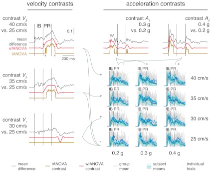
Data and contrast curves of TA EMG across 3 levels of acceleration and 4 levels of velocity. Gray traces: individual TA EMG traces. Blue traces: subject means for all perturbation levels. Black traces: mean difference curves across contrasts. Red traces: statistically significant identified contrast curves identified with wfANOVA. Yellow traces: statistically significant identified contrast curves identified with tANOVA. Left: contrasts V₃, V₂, and V₁ designating differences obtained between peak velocity levels. Top: contrasts A₂ and A₁ designating differences obtained between peak acceleration levels. Arrows in contrast V₃ designate onset and offset times for mean difference and contrast curves. Offset time for mean difference curve (1,210 ms) is beyond scale and not shown.

Unlike mean difference curves, contrast curves from wfANOVA only identified statistically significant differences in EMG during the IB time period due to increases in acceleration (Fig. 5, red traces, contrasts A₁ and A₂) and only in the PR period and later in the response due to increases in velocity (Fig. 5, red traces, contrasts V₁–V₃). These results confirmed previously described scaling relationships but without assuming analysis time bins a priori (cf. Welch and Ting 2009). Consistent with the previously described relationships, average wfANOVA acceleration contrast-curve onset times were 107 ± 6 and 88 ± 2 ms for TA and MG, respectively, whereas average wfANOVA velocity contrast-curve onset times were 331 ± 127 and 374 ± 93 ms for TA and MG, respectively. Acceleration contrast curves for TA and MG were primarily characterized by smooth features of ∼150 ms in width centered within the IB time period with magnitude increasing with the peak acceleration level (Fig. 5, red traces, A₁ and A₂ during IB). Velocity contrast curves were primarily characterized by wider (250 ms) smooth features within PR as well as some nonzero regions after the end of PR. Nonzero regions in the IB observed in the mean difference curves across velocity were not significantly different from zero (Fig. 5, V₃: black vs. red during IB). Unlike mean difference curves, which were nonzero for ∼1,000 ms, average feature widths in wfANOVA contrast curves were 273 ± 92 and 235 ± 121 ms in TA and MG, respectively.

Contrast curves from tANOVA identified statistically significant differences in time periods generally similar to wfANOVA but with features that were discontinuous functions of time with later onset times and smaller feature widths (Fig. 5, red vs. yellow traces). The discontinuities and sharp edges in tANOVA contrast curves were not observed in data nor in mean difference curves (Fig. 5, compare yellow traces to red or black) but were due to the large differences required at a single time point to reach statistical significance (Fig. 5, yellow tANOVA contrast V₃ during PR and contrast A₁ during IB). Thus, at smaller contrast levels, features of mean difference curves identified as significant by wfANOVA were rejected as insignificant by tANOVA due to reduced power. For example, small features identified late in the time course (Fig. 5, red vs. yellow traces at ∼550 ms, contrast V₁) by wfANOVA were not significantly different from zero in tANOVA due to reduced power. Like wfANOVA, tANOVA acceleration contrast-curve onset times were centered during IB (111 ± 8 ms, TA; 110 ± 6 ms, MG), and velocity contrast-curve onset times were centered during PR (303 ± 12 ms, TA; 399 ± 22 ms, MG). However, compared with wfANOVA, tANOVA contrast-curve onsets were delayed by 37 ± 35 ms (P < 0.02, t₇ = −2.94; Fig. 5, compare red errors and yellow arrows in contrast V₃). tANOVA contrast-curve offset times were advanced compared with wfANOVA (57 ± 88 ms), although this difference did not reach statistical significance (P > 0.10). The combination of delayed onset times and comparable offset times resulted in a significant overall reduction in feature width of 91 ± 96 ms in tANOVA compared with wfANOVA (P < 0.02, t₉ = 2.99).

Significant tests in wfANOVA and tANOVA.

Because of the compression properties of the wavelet transform, wfANOVA identified significantly fewer significant F tests than tANOVA, allowing post hoc tests to be performed at higher significance levels (Table 3). Considering the velocity and acceleration factors for TA and MG, the number of significant F tests was 40 ± 6 in wfANOVA vs. 160 ± 45 in tANOVA (P < 0.015, t₃ = 5.06). However, there was no significant difference between the percentage of initial F tests that led to significant post hoc tests in the two methods (25 ± 14%; matched t-test, P < 0.11, t₃ = 2.2). Considering the subject factor, all 512 time samples for tANOVA were significantly different, whereas 88 wavelet coefficients, including all 32 approximation-level wavelet coefficients, were significantly different for both TA and MG. Although we did not perform post hoc tests on subject factors, these differences demonstrate that there were differences in the mean waveform shape across subjects. We were nonetheless able to identify common effects of the acceleration and velocity factors on these waveforms.

Table 3.

Number of significant coefficients identified by wfANOVA and tANOVA for EMG responses to peak acceleration and velocity

		wfANOVA			tANOVA
Muscle	Factor	#F	P	#Post	#F	P	#Post
TA	V	35	0.0014	6	202	0.0002	63
	A	42	0.0012	12	97	0.0005	53
	S	88	0.0006		512	0.0001
MG	V	35	0.0014	6	173	0.0003	25
	A	47	0.0011	5	167	0.0003	45
	S	88	0.0006		512	0.0001

wfANOVA, wavelet-based functional ANOVA; tANOVA, ANOVA performed in the time domain; V, peak perturbation velocity; A, peak perturbation acceleration; S, subject.

^#F, number of coefficients corresponding to significant initial F tests; #Post, number of coefficients corresponding to significant post hoc tests.

Wavelet coefficients that varied significantly in post hoc tests were centered at time points consistent with the location of differences identified in contrast curves (Fig. 6). Across acceleration contrasts, 5 of 12 significant wavelet coefficients for TA and 3 of 5 coefficients for MG were centered within IB. In addition, some wavelet coefficients that varied with peak acceleration level were identified after the end of PR (TA, 2/12; MG, 2/5). Across velocity contrasts, the majority of significant wavelet coefficients (TA, 5/6; MG, 6/6) were centered after PR. Because wavelet coefficients centered later in the response also contribute substantial energy during earlier periods, the absence of significant wavelets during the PR period does not imply that there were no differences in waveforms during PR. For example, one of the wavelet coefficients that varied significantly with perturbation peak velocity for MG was centered at 567.5 ms after perturbation onset, well after the end PR (400 ms). However, the first nonzero sample of the wavelet corresponding to that coefficient was much earlier, at 216.7 ms, and the absolute magnitude of the wavelet waveform had increased to ∼20% of its maximum by 400 ms.

Fig. 6.

Distribution of significant wavelet coefficients in the time domain for all subjects. Bar plots are histograms of locations of significant wavelets in time for each muscle and factor. Vertical lines designate IB and PR time windows. MG, medial gastrocnemius.

Simulated EMG data.

wfANOVA revealed actual contrasts with high precision, superior to tANOVA, when applied to simulated EMG signals with nominal noise levels chosen to resemble experimental EMG data (Fig. 7, green traces, bottom right). At this noise level, the average r² values between original and noise-corrupted signals was 0.78 ± 0.06. Contrast curves identified by wfANOVA were similar to the known differences in the signals (Fig. 7, compare red vs. green traces; r² = 0.94 ± 0.08). As in the case of experimental data, tANOVA identified discontinuous contrast curves (Fig. 8, yellow trace, contrast V₂) and also failed to find any significant contrast between the lowest two levels of velocity (Fig. 7, compare red vs. yellow traces for V₁). The r² values between tANOVA contrast curves and actual contrast curves were lower than in wfANOVA (r² = 0.76 ± 0.43), although this difference was not statistically significant due to the small sample (paired t-test; P < 0.30, t₄ = 1.19). Compared with wfANOVA, tANOVA contrast curves also exhibited delayed onset time (43 ± 41 ms), advanced offset time (39 ± 46 ms), and decreased feature width (82 ± 84 ms), similar to the findings using experimental data. However, these differences did not reach statistical significance (P ≥ 0.079) due to the small sample size.

Fig. 7.

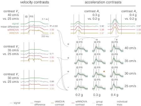
Comparison of waveforms representing mean differences across perturbation levels (mean difference curves; black) identified in simulated EMG data (gray) with contrast curves identified with wfANOVA (red) and tANOVA (yellow) and with veridical underlying signals (green). Legend as in Fig. 4. Numbers next to curves indicate r² values between identified mean difference curve or contrast curve and underlying signals. ★Combination of peak acceleration and peak velocity that was used to generate the remaining perturbation levels. au, Arbitrary units.

Fig. 8.

Simulated EMG signals and performance of wfANOVA vs. tANOVA across noise levels. A: changes in simulated EMG waveforms as n_G is increased across an order of magnitude. ★Waveform corresponding to model parameters used in Fig. 7. B: average (mean ± SD) r² values between noise-corrupted simulated EMG and uncorrupted signals as n_G is increased. C: r² values (median and range) between contrast curves identified by wfANOVA (black) and tANOVA (gray) and underlying signals as n_G is increased.

Across noise levels, wfANOVA performed superior to tANOVA in identifying contrast curves in simulated data with known temporal structure. Simulated EMG waveforms varied from almost noiseless (average r² between original and noise-corrupted signals 0.93 ± 0.02) to highly degraded (r² = 0.13 ± 0.07; Fig. 8, A and B). As expected, both algorithms had reduced ability to identify significant features of contrast curves as noise level increased. However, wfANOVA was more tolerant to noise (Fig. 8C). For example, at the highest noise level, wfANOVA identified significant contrasts at levels V₂, A₁, and A₂, whereas tANOVA identified significant contrasts only at level A₂. Across noise levels, wfANOVA was able to reveal better the actual contrast curves than tANOVA as measured by r² (median ± interquartile range: 0.92 ± 0.87, wfANOVA; vs. 0.29 ± 0.90, tANOVA; P < 10⁻⁷; Wilcoxon paired signed-rank test), onset time error (33 ± 61 vs. 57 ± 100 ms; P < 10⁻⁵), offset time error (47 ± 95 vs. 54 ± 86; P < 10⁻⁴), and feature width error (99 ± 367 vs. 178 ± 428; P < 10⁻⁷).

DISCUSSION

Here, we developed a novel method to compare statistically the shapes of waveforms that are functions of time that could be applied to many types of neurophysiological and other data. The technique can be used to identify temporal features characterizing the differences between waveforms across conditions that may not appear to be statistically significant due to multiple comparisons required across time points and that are abolished when analyzing large time bins. Such challenges are observed widely across neurophysiological and kinematic data, which are functions of time, and could be equally useful in the analysis of EMGs, reflex responses, kinematics, or neural firing rates. The method can also be extended by using different statistical procedures on the wavelet coefficients.

An advantage of wfANOVA is that no time windows need be assumed, removing the bias of the experimenter and possibly aiding in data discovery. The timing of significant differences in the contrast curves identified using wfANOVA were consistent with our previous analysis in which we selected time windows a priori based on previous knowledge, a proposed hypothesis, and trial and error (Welch and Ting 2009). Therefore, using wfANOVA can be used to identify the time windows of interest without prior knowledge or bias. Of course, this approach carries with it the burden of carefully controlling for false positives, which has been a subject of controversy in the neuroimaging literature (Bennett et al. 2009). We consider our implementation of wfANOVA conservative in that it uses a Bonferroni procedure to control the familywise error rate. Other approaches, such as false discovery rate controls, are available and have been applied to neuroimaging data (Genovese et al. 2002).

wfANOVA further revealed that the magnitude of mean difference curves found by subtracting time traces was not a reliable predictor of statistically significant differences between conditions. In our data set, we were able to reveal that some very small features were statistically significant, whereas larger ones that presumably had more variability were not statistically significant. As an example, our data showed small statistically significant features with changes in acceleration in a time period that we did not analyze in the prior study (Fig. 5, e.g., contrasts A₁ and A_2, bumps in red curve just before 1st vertical line). These differences likely reflect scaling of short-latency stretch reflex activity, which has been previously shown to be active during this time period (Carpenter et al. 1999; Gollhofer et al. 1989), starting ∼50 ms earlier than the long-latency response that was the focus of our prior study (Welch and Ting 2009). Thus wfANOVA can reveal meaningful contrasts across conditions that may not be apparent in visual inspection due to feature size, potentially providing novel insight into underlying neural mechanisms.

One primary difference between our approach and wavelet-domain statistical techniques applied previously to neuroimaging data is that we apply the wavelet transform to all data replicates within and across conditions rather than averaging data within each condition or subject before conversion to the wavelet domain. In addition, we focus on variations in the temporal rather than spatial domain. In many cases, wavelet-domain statistical analysis is used in medical imaging data as a “denoising” filter to estimate the underlying signals from multiple replicates of data with extremely low signal-to-noise ratio (Dinov et al. 2005; Fadili and Bullmore 2004; Raz and Turetsky 1999; Ruttimann et al. 1998; Unser and Aldroubi 1996). Because neuroimaging signals, particularly functional MRI (fMRI), tend to be noisy and of small magnitude, with signal intensity changes close to scan-to-scan variability, prior techniques first obtained averaged fMRI data for each subject within each experimental condition before performing the wavelet transformation (Raz and Turetsky 1999; Ruttimann et al. 1998) and performed statistical tests on a subset of wavelet coefficients at prespecified levels of detail to increase statistical power. Because the signal-to-noise ratio is much less problematic in EMG signals, we were able to apply directly the wavelet transformation to all replicates of EMG collected and to perform ANOVA on all wavelet coefficients without any a priori assumptions about their importance.

We performed some initial analyses suggesting that there is little benefit to prefiltering data by thresholding wavelet coefficients before performing ANOVA and that, further, such procedures can introduce unwanted artifacts. To test this idea, we reanalyzed experimental data from muscle TA presented in results with the addition of an initial thresholding procedure. In our reanalysis, we applied a hard threshold rule before performing ANOVA and post hoc tests on wavelet coefficients. Wavelet coefficients for which the grand mean of the wavelet transform magnitude was below a threshold corresponding to the 50th, 90th, or 99th percentile of observed wavelet coefficient magnitudes (Fig. 9A) were set to 0. Reconstructed waveforms at the 50th percentile threshold were similar to the original data (r² ≈ 0.99; Fig. 9B) and almost doubled the critical value that could be used in the post hoc tests, nominally increasing power. However, there were no practical benefits to this power increase because the number of significant post hoc tests remained unchanged. Thresholding at the 90th percentile (r² ≈ 0.90) introduced a small negative-going artifact in the signal before EMG onset (Fig. 9B, 2nd to top trace) and decreased the number of significant post hoc tests by 25%. At the 99th percentile threshold, waveforms were considerably smoothed (r² = 0.45 ± 0.19), and the negative-going artifacts were introduced well before EMG onset, at latencies of ∼80 ms. Increased threshold levels also led to the introduction of artifacts in identified contrast curves (Fig. 9C; note that negative bump in contrast V₁ that is apparent at lower threshold levels is absent at 99th percentile threshold). Although many more sophisticated thresholding procedures exist and could be beneficial (Donoho and Johnstone 1994; Donoho et al. 1995), more research is required to identify recommended practices.

Fig. 9.

Results of initial thresholding of small wavelet coefficients. A: example wavelet transform magnitude 〈|Y(w)|〉 with threshold levels indicated. The r² values (means ± SD) were calculated for all individual TA EMG trials before and after thresholding for each threshold level. B: example of an individual TA EMG waveform as thresholding is applied. Vertical lines indicate IB and PR periods. Because of the compression properties of the wavelet transform, there are minimal changes in the waveform until the highest level of thresholding (99%; top purple trace) is applied. C: wfANOVA contrast curves identified at additional features at increased threshold levels. As threshold is increased (left to right), overall wfANOVA contrast-curve shapes are retained until the highest level of thresholding. The r² values were computed between the thresholded contrast curves and the original contrast curve.

General applications.

Although our implementation of wfANOVA presented a particular statistical model, the underlying concept of performing statistical inference in the wavelet domain and then transforming back to time domain is general to ANOVA and other statistical tests. Here, we presented one particular implementation of wfANOVA based on a fixed-effects ANOVA model. However, interaction effects could also be included in the ANOVA model. Similarly, MANOVA hypothesis tests for different blocks of wavelet coefficients have been suggested for fMRI data (Raz and Turetsky 1999). False discovery rate controls (Benjamini and Hochberg 1995) could also be applied in place of the Bonferroni procedures presented here.

Statistical inference can also be applied to transforms other than the wavelet transform that involve a common orthogonal basis for all waveforms under analysis. It is possible to perform analyses similar to wfANOVA using the discrete Fourier transform rather than the discrete wavelet transform (Fan and Lin 1998), although the Fourier transform typically provides a less compact description of biomedical signals. However, although wavelet packets can provide a more compact description of EMG signals (Hart and Giszter 2004) than either the discrete Fourier transform or the discrete wavelet transform, they cannot be used in wfANOVA without additional constraints on the packet tree. Depending on the way the packet tree is structured, each waveform may be represented by a unique set of functions, prohibiting comparisons across waveforms. An alternative could be to represent all waveforms by a common overcomplete basis; however, this would increase the number of comparisons.

Finally, wfANOVA may also be useful in comparing a single observation with a population average such as when comparing data from an impaired individual with controls or comparing a model prediction with experimental data. Currently, such comparisons are difficult in part because r² values may penalize high-frequency components while ignoring differences in overall waveform shape. Differences in the high-frequency content are particularly pronounced when comparing model predictions and experimental data, and multiple goodness-of-fit metrics (such as r² and variance accounted for) may be required to reduce sensitivity to noise (Ting and Chvatal 2011). Another approach is to examine whether the model predictions fall within standard deviations or confidence intervals generated from data on a per-sample basis, similar to the tANOVA approach presented here. However, this approach leads to problems of multiple comparisons similar to those described earlier for tANOVA because statistical tests designed for single values are not well-suited to comparing waveforms or curves (Fan and Lin 1998; Lund et al. 2011). To address this issue, the wfANOVA framework could be modified to identify better which features of a single model prediction or experimental measurement are significantly different from a set of control data and which are not.

GRANTS

National Institute of Neurological Disorders and Stroke Grant NS-058322 supported this work.

DISCLOSURES

No conflicts of interest, financial or otherwise, are declared by the authors.

ENDNOTE

At the request of the authors, readers are herein alerted to the fact that additional materials related to this manuscript may be found at the institutional web site of the authors, which at the time of publication they indicate is: https://neurolab.gatech.edu/wp/wp-content/uploads/2012/08/wfANOVAdemo.zip. These materials are not a part of this manuscript and have not undergone peer review by the American Physiological Society (APS). APS and the journal editors take no responsibility for these materials, the web site address, or any links to or from it.

AUTHOR CONTRIBUTIONS

J.L.M., T.D.J.W., B.V., and L.H.T. conception and design of research; J.L.M. and T.D.J.W. analyzed data; J.L.M. and L.H.T. interpreted results of experiments; J.L.M. prepared figures; J.L.M. drafted manuscript; J.L.M., T.D.J.W., B.V., and L.H.T. edited and revised manuscript; J.L.M., T.D.J.W., B.V., and L.H.T. approved final version of manuscript; T.D.J.W. performed experiments.

REFERENCES

- Abramovich F, Antoniadis A, Sapatinas T, Vidakovic B. Optimal testing in functional analysis of variance models. Int J Wavelets Multiresol Inf Proc 2: 323–349, 2004 [Google Scholar]
- Angelini C, Vidakovic B. Some novel methods in wavelet data analysis: wavelet ANOVA, F-test shrinkage, and Γ-minimax wavelet shrinkage. In: Wavelets and Their Applications, edited by Krishna M, Radha R, Thangvelu S. New Delhi: Allied Publishers, 2003, p. 31–45 [Google Scholar]
- Benjamini Y, Hochberg Y. Controlling the false discovery rate: a practical and powerful approach to multiple testing. J R Stat Soc Series B Stat Methodol 57: 289–300, 1995 [Google Scholar]
- Bennett CM, Wolford GL, Miller MB. The principled control of false positives in neuroimaging. Soc Cogn Affect Neurosci 4: 417–422, 2009 [DOI] [PMC free article] [PubMed] [Google Scholar]
- Carpenter MG, Allum JH, Honegger F. Directional sensitivity of stretch reflexes and balance corrections for normal subjects in the roll and pitch planes. Exp Brain Res 129: 93–113, 1999 [DOI] [PubMed] [Google Scholar]
- Cohen A, Kovacevic J. Wavelets: the mathematical background. Proc IEEE 84: 514–522, 1996 [Google Scholar]
- Dinov I, Boscardin J, Mega M, Sowell E, Toga A. A wavelet-based statistical analysis of fMRI data. Neuroinformatics 3: 319–342, 2005 [DOI] [PubMed] [Google Scholar]
- Donoho DL, Johnstone IM. Threshold selection for wavelet shrinkage of noisy data (Abstract). In: Engineering in Medicine and Biology Society. Engineering Advances: New Opportunities for Biomedical Engineers. Proceedings of the 16th Annual International Conference of the IEEE Baltimore, MD: November 3–6, 1994, p. A24–A25 [Google Scholar]
- Donoho DL, Johnstone IM, Kerkyacharian G, Picard D. Wavelet shrinkage: asymptopia? J R Stat Soc Series B Stat Methodol 57: 301–369, 1995 [Google Scholar]
- Fadili MJ, Bullmore ET. A comparative evaluation of wavelet-based methods for hypothesis testing of brain activation maps. Neuroimage 23: 1112–1128, 2004 [DOI] [PubMed] [Google Scholar]
- Fan J, Lin SK. Test of significance when data are curves. J Am Stat Assoc 93: 1007–1021, 1998 [Google Scholar]
- Fang J, Agarwal GC, Shahani BT. Decomposition of multiunit electromyographic signals. IEEE Trans Biomed Eng 46: 685–697, 1999 [DOI] [PubMed] [Google Scholar]
- Flanders M. Choosing a wavelet for single-trial EMG. J Neurosci Methods 116: 165–177, 2002 [DOI] [PubMed] [Google Scholar]
- Frigon A. Effect of rhythmic arm movement on reflexes in the legs: modulation of soleus H-reflexes and somatosensory conditioning. J Neurophysiol 91: 1516–1523, 2004 [DOI] [PubMed] [Google Scholar]
- Genovese CR, Lazar NA, Nichols T. Thresholding of statistical maps in functional neuroimaging using the false discovery rate. Neuroimage 15: 870–878, 2002 [DOI] [PubMed] [Google Scholar]
- Gollhofer A, Horstmann GA, Berger W, Dietz V. Compensation of translational and rotational perturbations in human posture: stabilization of the centre of gravity. Neurosci Lett 105: 73–78, 1989 [DOI] [PubMed] [Google Scholar]
- Harris CM, Wolpert DM. Signal-dependent noise determines motor planning. Nature 394: 780–784, 1998 [DOI] [PubMed] [Google Scholar]
- Hart CB, Giszter SF. Modular premotor drives and unit bursts as primitives for frog motor behaviors. J Neurosci 24: 5269–5282, 2004 [DOI] [PMC free article] [PubMed] [Google Scholar]
- Hiebert GW, Gorassini MA, Jiang W, Prochazka A, Pearson KG. Corrective responses to loss of ground support during walking. II. Comparison of intact and chronic spinal cats. J Neurophysiol 71: 611–622, 1994 [DOI] [PubMed] [Google Scholar]
- Huber C, Nüesch C, Göpfert B, Cattin PC, von Tscharner V. Muscular timing and inter-muscular coordination in healthy females while walking. J Neurosci Methods 201: 27–34, 2011 [DOI] [PubMed] [Google Scholar]
- Ivanenko YP, Cappellini G, Dominici N, Poppele RE, Lacquaniti F. Coordination of locomotion with voluntary movements in humans. J Neurosci 25: 7238–7253, 2005 [DOI] [PMC free article] [PubMed] [Google Scholar]
- Kumar DK, Pah ND, Bradley A. Wavelet analysis of surface electromyography to determine muscle fatigue. IEEE Trans Neural Syst Rehabil Eng 11: 400–406, 2003 [DOI] [PubMed] [Google Scholar]
- Lund ME, de Zee M, Rasmussen J. Comparing calculated and measured curves in validation of musculoskeletal models (Abstract). In: XIII International Symposium on Computer Simulation in Biomechanics Leuven, Belgium: 2011 [Google Scholar]
- Mushiake H, Inase M, Tanji J. Neuronal activity in the primate premotor, supplementary, and precentral motor cortex during visually guided and internally determined sequential movements. J Neurophysiol 66: 705–718, 1991 [DOI] [PubMed] [Google Scholar]
- Ostlund N, Yu J, Karlsson JS. Adaptive spatio-temporal filtering of multichannel surface EMG signals. Med Biol Eng Comput 44: 209–215, 2006 [DOI] [PubMed] [Google Scholar]
- Ramsay JO, Silverman BW. Functional Data Analysis. New York; Berlin: Springer, 2005 [Google Scholar]
- Raz J, Turetsky B. Wavelet ANOVA and fMRI. In: Proceedings of the SPIE Conference on Mathematical Imaging: Wavelet Applications in Signal and Image Processing VII Denver, CO: 1999 [Google Scholar]
- Ren X, Hu X, Wang Z, Yan Z. MUAP extraction and classification based on wavelet transform and ICA for EMG decomposition. Med Biol Eng Comput 44: 371–382, 2006 [DOI] [PubMed] [Google Scholar]
- Ruttimann UE, Unser M, Rawlings RR, Rio D, Ramsey NF, Mattay VS, Hommer DW, Frank JA, Weinberger DR. Statistical analysis of functional MRI data in the wavelet domain. IEEE Trans Med Imaging 17: 142–154, 1998 [DOI] [PubMed] [Google Scholar]
- Sokol RR, Rohlf FJ. Biometry. W. H. Freeman, 1981 [Google Scholar]
- Strang G. Wavelets and dilation equations: a brief introduction. SIAM Rev Soc Ind Appl Math 31: 614–627, 1989 [Google Scholar]
- Stulen FB, De Luca CJ. Frequency parameters of the myoelectric signal as a measure of muscle conduction velocity. IEEE Trans Biomed Eng 28: 515–523, 1981 [DOI] [PubMed] [Google Scholar]
- Ting LH, Chvatal SA. Decomposing muscle activity in motor tasks: methods and interpretation. In: Motor Control: Theories, Experiments, and Applications, edited by Danion F, Latash ML. New York: Oxford Univ. Press, 2011 [Google Scholar]
- Tresch MC, Cheung VC, d'Avella A. Matrix factorization algorithms for the identification of muscle synergies: evaluation on simulated and experimental data sets. J Neurophysiol 95: 2199–2212, 2006 [DOI] [PubMed] [Google Scholar]
- Unser M, Aldroubi A. A review of wavelets in biomedical applications. Proc IEEE 84: 626–638, 1996 [Google Scholar]
- von Tscharner V. Intensity analysis in time-frequency space of surface myoelectric signals by wavelets of specified resolution. J Electromyogr Kinesiol 10: 433–445, 2000 [DOI] [PubMed] [Google Scholar]
- Wakeling JM, Horn T. Neuromechanics of muscle synergies during cycling. J Neurophysiol 101: 843–854, 2009 [DOI] [PubMed] [Google Scholar]
- Welch TD, Ting LH. A feedback model explains the differential scaling of human postural responses to perturbation acceleration and velocity. J Neurophysiol 101: 3294–3309, 2009 [DOI] [PMC free article] [PubMed] [Google Scholar]
- Valero-Cuevas FJ, Venkadesan M, Todorov E. Structured variability of muscle activations supports the minimal intervention principle of motor control. J Neurophysiol 102: 59–68, 2009 [DOI] [PMC free article] [PubMed] [Google Scholar]
- Vidakovic B. Wavelet-based functional data analysis: theory, applications and ramifications. In: Proceedings of the 3rd Pacific Symposium on Flow Visualization and Image Processing Maui, HI: 2001 [Google Scholar]