Mapping Tumor Hypoxia In Vivo Using Pattern Recognition of Dynamic Contrast-enhanced MRI Data^,

Abstract

In solid tumors, hypoxia contributes significantly to radiation and chemotherapy resistance and to poor outcomes. The “gold standard” pO₂ electrode measurements of hypoxia in vivo are unsatisfactory because they are invasive and have limited spatial coverage. Here, we present an approach to identify areas of tumor hypoxia using the signal versus time curves of dynamic contrast-enhanced magnetic resonance imaging (DCE-MRI) data as a surrogate marker of hypoxia. We apply an unsupervised pattern recognition (PR) technique to determine the differential signal versus time curves associated with different tumor microenvironmental characteristics in DCE-MRI data of a preclinical cancer model. Well-perfused tumor areas are identified by rapid contrast uptake followed by rapid washout; hypoxic areas, which are regions of reduced vascularization, are identified by delayed contrast signal buildup and washout; and necrotic areas exhibit slow or no contrast uptake and no discernible washout over the experimental observation. The strength of the PR concept is that it captures the pixel-enhancing behavior in its entirety—during both contrast agent uptake and washout—and thus, subtleties in the temporal behavior of contrast enhancement related to features of the tumor microenvironment (driven by vascular changes) may be detected. The assignment of the tumor compartments/microenvironment to well vascularized, hypoxic, and necrotic is validated by comparison to data previously obtained using complementary imaging modalities. The proposed novel analysis approach has the advantage that it can be readily translated to the clinic, as DCE-MRI is used routinely for the identification of tumors in patients, is widely available, and easily implemented on any clinical magnet.

Introduction

The microenvironment in solid tumors is characterized by inadequate and heterogeneous perfusion, hyper-permeable vasculature, hypoxia, acidic extracellular pH, and nutrient deprivation [1]. Hypoxic tumors, often associated with a more aggressive tumor phenotype [2], are more resistant to chemotherapy or radiation therapy than well-vascularized, well-oxygenated tumors [1–4]. Thus, in vivo knowledge of the spatial distribution of hypoxia in tumors may provide prognostic information and can possibly improve treatment planning (e.g., intensity-modulated radiotherapy) or choice of anticancer drug regimen [4]. Current clinical and preclinical methods to measure hypoxia, reviewed in detail previously [3,5], include 1) invasive procedures, such as pO₂ electrode measurements, ex vivo immunohistochemistry of exogenous markers (pimonidazole, EF-5), or hypoxia-related proteins (hypoxia-inducible factor-1α, carbonic anhydrase IX, and osteopontin) on tumor biopsy samples, and 2) minimally or noninvasive in vivo procedures, such as positron emission tomography (PET) using exogenous, radioactive hypoxia tracers (¹⁸F-Fmiso, ¹⁸F-FAZA, and so on), magnetic resonance (MR) methods [blood oxygen level-dependent (BOLD), tissue oxygen level-dependent (TOLD), ¹⁹F MR relaxometry of perfluorocarbons], or electron paramagnetic resonance. Each of these methods has advantages and disadvantages in terms of its capability of measuring the spatial distribution of hypoxia in vivo and the confidence in the accuracy of the measurement. For example, assessing tumor hypoxia using biopsy samples suffers from inadequate sampling of the tumor and repeated sampling for assessing changes of tumor hypoxia during tumor progression or treatment is not practical. Assessing tumor hypoxia in vivo using PET requires the administration of a radioactive tracer and, thus, exposes patients to ionizing radiation. Further, although its sensitivity is excellent, PET has relatively coarse spatial resolution and provides limited anatomic information, requiring added-on computed tomography or MR imaging (MRI) [5–8]. Additionally, recent studies indicate that dynamic PET may be necessary to reliably identify hypoxic tumor regions, prolonging data collection and analysis [6,7]. Thus, there is currently no standard method in the clinical or pre-clinical setting to reliably image hypoxia in vivo [4,5].

Currently, dynamic contrast-enhanced (DCE)-MRI data are fitted pixel by pixel using pharmacokinetic models, such as, for example the Tofts model [9,10] which results in two parameters characterizing the dynamics of the pixel enchantment. The initial part of the DCE curve is characterized by K^trans, the volume transfer constant between plasma and extracellular extravascular space, whereas the contrast washout is characterized by k_ep, the rate constant between extracellular extravascular space and plasma. In this type of analysis, regional differences of pixel-enhancing behavior across a tumor area are typically separated by thresholding. This limits the ability to separate voxels featuring similar—albeit not the same—contrast uptake dynamics, as e.g., seen by Cho et al. for hypoxic and well-perfused, viable tumor areas [6]. To overcome this limitation, we present here an approach to identify areas of tumor hypoxia by analyzing the signal versus time curves of DCE-MRI data with an unsupervised pattern recognition (PR) technique. The strength of this concept is that it captures the pixel-enhancing behavior in its entirety—during both contrast agent uptake and washout—and thus, subtleties in the temporal behavior of contrast enhancement related to features of the tumor microenvironment (driven by vascular changes) may be detected. Additionally, analyzing the entire data set simultaneously rather than the individual pixel's signal versus time curves significantly increases the signal-to-noise ratio. The assignment of the resulting pattern to well vascularized, hypoxic, and necrotic tumor areas, respectively, has been validated by the data of Cho et al. [6].

DCE-MRI is widely available, relatively easy to implement, and already routinely used in the clinic. Implementing the described analysis procedures is straightforward, and the capability to decipher tumor heterogeneity can be readily translated to the clinic. This potentially will eliminate the need for additional invasive procedures lacking adequate spatial sampling (biopsies) or the serial exposure to radioactive tracers (PET) for assessing tumor hypoxia.

Materials and Methods

Description of Experimental Data

We analyzed previously obtained DCE-MRI data from four Dunning rat R3327-AT prostate cancer syngeneic tumors, labeled A to D based on their tumor volume: 478 mm³ (A), 744 mm³ (B), 870 mm³ (C), and 1230 mm³ (D) [6]. The results of our analysis are validated by a comparison to the results obtained previously from multimodality imaging data. The details regarding experimental design and data acquisition are described elsewhere [6].

Briefly, R3327-AT tumors, implanted subcutaneously on the right hind leg of Copenhagen rats, were imaged using a stereotactic fiduciary marker system permitting the coregistration of images obtained from different imaging modalities [6,11]. The animals underwent in vivo DCE-MRI (vascular perfusion/permeability) using the contrast agent gadolinium-diethylenetriamine pentaacetic acid (Gd-DTPA) and, subsequently, in vivo dynamic ¹⁸F-Fmiso PET (hypoxia) followed by staining of excised tumor sections with pimonidazole (hypoxia) and hematoxylin and eosin (H&E; necrosis) [6]. DCE-MRI data were acquired at 5.347-second temporal resolution for ∼2 minutes before Gd-DTPA injection, followed by ∼20-minute dynamic acquisition, resulting in 256 image sets (five tumor slices each). The voxel size was 0.273 x 0.273 x 0.79mm³ (0.059 mm³) with an 128 x 128 in-plane matrix and 35 mm x 35 mm field of view. For each tumor, ¹⁸F-Fmiso PET data from the dynamic acquisition were reconstructed, resulting in 45 to 49 time frames with a voxel size of 0.86 x 0.86 x 0.79 mm³ (0.58 mm³). For ex vivo analysis, images of 8-µm-thick pimonidazole and H&E-stained tumor sections, sampled at positions corresponding to the mid-slice of the MRI and PET image sets, were captured at 0.85 x 0.85 µm² in-plane resolution, depicting the spatial distribution of hypoxia and necrosis, respectively [6].

Principal Component Analysis

In the exploration of large data sets (here, DCE-MRI results in more than 1000 images for one experiment), principal component analysis (PCA) is an invaluable tool for the identification of the sources of largest variations, called principal components (PCs). Representing the data in a lower dimensional space defined by the significant PCs allows for easier interpretation of the dynamics in the data [12,13].

Here, V(X, t) denotes a data matrix with the individual signal versus time curves in its rows (X depicting spatial location and t depicting time). PCA decomposes V into the product of 1) the PCs, which are orthonormal and ordered by decreasing amounts of variability in the data they represent, and 2) the scores or magnitudes, which are the weights of each PC in the original data. For instance, in DCE-MRI data from an entirely homogeneous tissue/organ, all signal versus time curves will have an almost identical (within the noise of the measurement) temporal pattern and PCA will yield a first PC as the normalized curve of this pattern, while the second and higher PCs will be noise related. The entire data set from this homogeneous tissue/organ can be represented without loss of information as the product of the first PC and its scores. When DCE-MRI is acquired from a heterogeneous sample, PCA will yield multiple significant signal-related PCs, matching the number k of sources (tissues/compartments with significant contribution to entire region of interest) for different signal versus time curves.

PCA is a standard routine in series of commercial and open source software, such as MATLAB, SAS, SPSS, R, and so on. In this particular implementation, no mean centering of the data is required and the PCs and their scores are obtained through singular value decomposition of the data covariance matrix rather than the data correlation matrix [13].

Pattern Recognition

While PCs are useful mathematical constructs for initial exploration of the data and to obtain the number k of independent basic temporal curves characterizing DCE-MRI data, the temporal shapes of the orthonormal PCs cannot be directly interpreted in terms of signal versus time DCE-MRI curves. Thus, constrained nonnegative matrix factorization (cNMF) [14], an unsupervised PR algorithm, is applied to V, seeking k solutions of basic temporal curves. cNMF assumes that each image in the DCE-MRI series represents k tissue types with individually associated basic signal versus time curve shapes, that is, cNMF seeks a representation of V as a product of k basic contrast signatures S(t) and their weights W. Mathematically, this would be expressed as V ∼ W(X)x S(t) under the constraint that the elements of W and S are nonnegative (note that the k basic contrast signatures obtained by cNMF are not orthonormal like the k significant PCs). The weights W quantify the contribution of each of the k patterns to the final uptake pattern in any given voxel, thus accounting for subvoxel contrast uptake behavior. That means this approach is not only capable of separating voxels predominantly following one given pattern but also identify voxels that have significant contributions from more than one pattern, effectively increasing the spatial resolution of the data.

cNMF belongs to the class of blind source separation/independent component analysis methods, and a variety of algorithms for the nonnegative decomposition of data are publicly available [15]. cNMF was introduced primarily for fast recovery of biochemically meaningful spectral patterns in three-dimensional magnetic resonance spectroscopic imaging data [14]. The algorithmic and computational details of NMF [16,17] and cNMF [14,18,19] have been described previously.

Results

PR Approach

Figure 1 illustrates the workflow of our analysis procedure, using data from animal B: 256 image sets (each 128 x 128 x 5 pixels) are organized in a two-dimensional space-time data matrix V(X, t), where X depicts the spatial location of the pixel. The mean of the 23 pre-contrast image sets is subtracted from the data set. A representative array of signal versus time curves depicts the shape differences of the curves in the tumor region, reflecting the heterogeneity of underlying tumor tissue features (Figure 1A). Three distinct temporal patterns of tumoral signal versus time curves are indicated by colored boxes (Figure 1A, from left to right): blue—continuous slow uptake; green—faster uptake and some washout; and red—rapid uptake and fast washout. On the basis of their shape [6] and image location, these curves are most likely associated with necrotic, hypoxic, and well-vascularized/highly permeable tumor tissues, respectively. Note that we will subsequently refer to the well-vascularized/highly permeable tumor areas as “well perfused.”

Figure 1.

Analysis workflow illustrated for DCE-MRI data from a Dunning R3327-AT prostate tumor model. (A) A representative array of signal versus time curves from a tumor region and adjacent muscle tissue, depicted by the green box on a representative T₁-weighed MR image on the right, is shown. The color boxes indicate three differential temporal patterns in the tumor (from left to right): blue—continuous slow uptake; green—faster uptake and some washout; red—rapid contrast uptake and fast washout. On the basis of their temporal shape [6], as well as their image location, these curves are most likely associated with necrotic, hypoxic, and well-perfused tumors, respectively. (B) Left: First four PCs, together with their fractional contribution to the data variability. Right: Spatial distribution of the magnitude of the corresponding PC scores in the five image slices. (C) PCA applied only to the DCE data from pixels within the tumor. Left: First four PCs. Right: Spatial distribution of the magnitude of the corresponding PCs in a representative central tumor slice (note that the PCA was carried out on the entire data set). (D) cNMF analysis of the data seeking three solutions. Left: Basic signal versus time curves, S(t). Right: Spatial distribution of the corresponding weights, W, in the five tumor slices.

PCA was applied to V, and the first four PCs from the DCE-MRI data of animal B and their corresponding weight/amplitude images are presented in Figure 1B. The numbers next to each PC indicate the percent variability in V each PC accounts for. The results illustrate that there are three signal-related PCs, while the fourth and higher (not displayed) PCs are noise related. This indicates that the data are composed of three basic temporal curves. From the corresponding magnitude images, it can be inferred that almost all contrast-related changes occur within the tumor, although signal enhancement can also be seen in the surrounding muscle. Guided by the map of the first PC, the tumor area is outlined manually, and PCA is applied only to the signal-to-time curves from tumor pixels (Figure 1C). Again, the first three PCs explain more than 99.9% of total variability in V. Note that the PCs contain both positive and negative segments, limiting their side-by-side comparison with experimental signal versus time curves.

cNMF is applied to the data matrix V, seeking three solutions (k = 3), and the results are represented in Figure 1D: the basic signal versus time curves S(t) are on the left and the spatial distribution of their corresponding weights W(X)in V is on the right. The top pattern is characterized by fast Gd-DTPA uptake and washout, with the highest intensities in the corresponding weights being close to the tumor surface. The middle curve and its corresponding weight image depict delayed signal buildup and washout, indicative of reduced vascularization. Compared to the other two patterns, the third pattern features the slowest time-dependent signal increase with no observable washout over the time course with the highest weighting in central tumor areas.

A detailed mathematical description of the workflow is described in the Supplementary section.

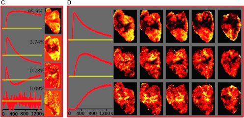
The PCA/cNMF analysis of DCE-MRI data from three other tumors are presented in Figure 2. PCA of the smallest tumor A reveals that almost the entire variability can be represented by one PC (Figure 2A). The shape of the first PC, which approximates the normalized average of the tumoral signal versus time curves, is notably different than that of the first PCs in Figure 1, B and C. It is similar to the first cNMF curve in Figure 1D: the signal increases at fastest as a result of rapid Gd-DTPA uptake followed by rapid washout, which is reflected in the temporal pattern. One of the most likely explanations is that this particular tumor is quite homogeneous and well vascularized. Consequently, cNMF failed to decompose the data set into multiple temporal patterns. The second PC in this tumor (Figure 2A, second row), accounting for only 0.5% of variability in this data set, displays the features of very fast contrast agent uptake and washout (a characteristic found in large vessels [20]) and, based on its temporal shape and location throughout the slices, may represent a feeding vessel for this tumor.

Figure 2.

PR analysis. (A) Left: First four PCs from DCE-MRI data from the smallest tumor A in the analyzed series (478 mm³). The first PC explains more than 99% of the variability, suggesting high level of homogeneity in the tumor microenvironment. Right: Spatial distribution of the magnitude of the corresponding PC scores in the five tumor slices. (B) cNMF applied to DCE-MRI data from tumor C (870 mm³). Only the first 145 time points from the DCE series (∼775 seconds) were analyzed, as PCA analysis of this tumor (data not shown) indicated that there was an interruption in the PC curves around the 145th time point, possibly because of movement. Left: Basic signal versus time curves S(t). Right: Spatial distribution of the corresponding weights W in the five tumor slices. (C) cNMF applied to DCE-MRI data from tumor D (1230 mm³). Left: Basic signal versus time curves S(t). Right: Spatial distribution of the corresponding weights W in the five tumor slices.

The cNMF curves obtained from tumors C and D (Figure 2, B and C) have almost identical shapes to those from animal B (Figure 1D). In addition, the shapes of the cNMF-identified temporal curves are similar to manually selected, representative signal versus time curves for perfused, hypoxic, and necrotic areas, respectively, published in Cho et al. [6].

Relationship between cNMF Curve Shapes and the Tumor Microenvironment

In Figure 3, A and C, respectively, the weights of the differential signal versus time patterns (cNMF curves) are presented as composite color maps for two representative tumor tissue slices from animals B and D, with red depicting fast contrast agent uptake and washout, green depicting delayed contrast agent uptake and washout, and blue and black areas depicting slow or no contrast agent uptake, respectively. Voxels that have significant contributions from more than one pattern, as quantified by the weight of each differential signal versus time pattern, are depicted by the mixing of their respective colors. For example, a voxel with significant contributions from the red and blue channels would be depicted as a corresponding purple shade. The individual color components of these maps are compared in Figure 3, B and D, to maps depicting well-vascularized, necrotic, and hypoxic tumor areas, respectively, which were obtained previously from complementary imaging modalities by Cho et al. [6].

Figure 3.

Correlation of contrast agent uptake patterns as determined by PCA/cNMF analysis of DCE-MRI data to tissue microenvironments as determined by other imaging modalities. (A, C) Composite color images of signal versus time patterns (cNMF curves) in individual tumors B (A, tumor volume = 744 mm³) and D (C, tumor volume = 1230 mm³). The colors represent the weights of the first (red), second (green), and third (blue) cNMF curves, as displayed in Figures 1D and 2C for the two tumors, respectively. (B, D) The spatial distribution of the three temporal patterns compared to the spatial distribution of well-perfused, hypoxic, and necrotic areas, respectively, as identified previously by other imaging modalities [6]. The red cNMF map agrees well with the corresponding Ak_ep map estimated from the DCE-MRI data and represents well-vascularized areas. The blue pattern, including the black core of the tumor, overlaps with the areas of necrosis, as determined from corresponding H&E-stained tissue sections. The hypoxic areas in these tumors previously obtained from the late ¹⁸F-Fmiso slope data (in vivo) and pimonidazole-stained tissue sections (ex vivo) [6] correspond well to the distribution in the green map. Green and red arrows indicate hypoxic areas adjacent to necrotic and well-vascularized areas, respectively. ¹⁸F-Fmiso maps, as well as the images of the H&E- and pimonidazole-stained tumor tissue sections, were adapted with permission from Cho et al. [6].

1. Areas of fast contrast uptake and washout (voxels in red) appear to be spatially well correlated with the distributions of high Ak_ep values in Cho et al. [6]. The Ak_ep map has been obtained by fitting the contrast versus time curves in each voxel using the two-compartment model by Hoffmann et al. [21]. In this model, Ak_ep is the product of amplitude A (degree of relative MR signal enhancement) and exchange rate kep (related to the rate of MR signal increase) and is considered an approximate measure of vascular perfusion and permeability of the tumor tissue [21]. Thus, the first cNMF curve is characteristic of well-perfused tumor tissue.

2. Previously, tumor necrotic areas were identified ex vivo from H&E-stained tissue sections of these tumors that were aligned to the corresponding in vivo DCE-MRI slices [6] (Figure 3, B and D). The distribution of necrotic areas appears to be spatially well correlated with tumor areas characterized by the third cNMF curve shape, that is, areas of low or no contrast uptake as identified in vivo from DCE-MRI data (voxels in blue and black; Figure 3, B and D).

3. The remaining tumor areas (voxels in green), characterized by the second cNMF curve shape, are compared to the corresponding in vivo PET images depicting the slope map of tumoral ¹⁸F-Fmiso time-activity curves and images of corresponding ex vivo pimonidazole-stained tissue sections (Figure 3, B and D). In the PET data, hypoxic areas are identified by the positive slope of the late portion of the ¹⁸F-Fmiso curves and are related to the continuing accumulation and lack of clearance of the hypoxia tracer, while on tissue sections, pimonidazole-stained areas are considered hypoxic [6].

While the total hypoxic areas identified in the tumor slice by all modalities (DCE-MRI, ¹⁸F-Fmiso PET, and pimonidazole) appear comparable, the intensity scales for the different imaging modalities (Figure 3, B and D) are different. This can be explained when considering a number of method-related features directly affecting the respective intensity scale: 1) The green in the hypoxic maps obtained from the unsupervised PR analysis of the DCEMRI data is weighted to represent how much of each pattern contributes to each pixel, that is, bright green are voxels following predominantly the shape of delayed contrast uptake and washout, while faint green voxels are a mixture of more than one pattern; 2) in contrast, the ¹⁸F-Fmiso slope and pimonidazole maps result from the uptake and metabolism of the respective 2-nitroimidazole, which not only depends on oxygen level but also on tracer concentration, perfusion, cell viability, and cellular nitroreductase activities [22]. Therefore, hypoxic areas adjacent to well-vascularized voxels will appear more intense in the various images than hypoxic areas that are closer to necrotic areas, as more of the nitroimidazole reaches cells in the former than the latter. This is readily visible in the faint green staining of the area immediately adjacent to a necrotic area (green arrows, Figure 3B, Ak_ep, PIMO), which is not well vascularized, while an intense green area (red arrows, Figure 3B, Ak_ep, PIMO) appears to be a hypoxic area adjacent to a well-vascularized area. This also means that the intensity of the ¹⁸F-Fmiso slope map is affected by vascular perfusion/permeability, leading to higher slope values for hypoxic regions close to well vascularized areas and lesser slope values in those areas that are adjacent to necrosis and, thus, poorly vascularized (green arrows, Figure 3B, ¹⁸F-Fmiso vs Ak_ep).

While previously the three microenvironments were manually selected on the basis of DCE-MRI, H&E, pimonidazole, and late ¹⁸F-Fmiso slope images (shown for comparison in Figure 3, B and D) [6], in the approach described here tissue segmentation was achieved automatically and objectively on the basis of the differential temporal patterns in DCE-MRI alone. The color depiction facilitates the comparison of our results to the images acquired by Cho et al. [6] using four image modalities.

Visualization and Quantification of Tumor Microenvironments/Compartments

For the four tumors analyzed, the weights of the differential signal versus time patterns are presented in Figure 4A (in order of increasing tumor size) as composite color maps depicting well-vascularized/perfused, hypoxic, and necrotic areas, respectively, in red, green, and blue/black. The smallest tumor (tumor A, top) is entirely well perfused. For the larger tumors, the images are consistent with our basic understanding of tumor architecture and physiology: the tumor center is mostly necrotic, with the hypoxic compartment closely enveloping the necrotic core and the well-vascularized/perfused components at the periphery. As the contrast agent penetrates the necrotic tissues via diffusion, only areas adjacent to the hypoxic compartment are depicted in blue; the black tumor areas, unreached by Gd-DTPA, are also part of the necrotic tumor areas. Qualitatively, it is apparent that the fraction of well-vascularized/perfused tumor area decreases while the necrotic tumor compartment increases with tumor size. Notably, multiple extensions of the hypoxic compartment penetrate the well-perfused regions, depicting areas less effectively supplied with oxygen because of reduced or dysfunctional vasculature.

Figure 4.

Summary of PR analysis. (A) Composite color images of individual tumor subtissue features, as identified by PR analysis. The presented images in the five slices in tumors A, B, C, and D refer to perfused (red), hypoxic (green), and necrotic (blue/black) tissues. Note that the black areas adjacent to the blue voxels are also part of the necrotic core. The tumor sizes are 478 mm³ (A), 744 mm³ (B), 870 mm³ (C), and 1230 mm³ (D). (B) Fractions of the three tissue features in the four tumors.

For quantification, image pixels above background are labeled well perfused, hypoxic, or necrotic on the basis of which one of the three patterns has maximum weight, and their fractional area was calculated as percentage tumor area (Figure 4B). Areas of low-contrast signal (less than 25% of the maximum intensity simultaneously in the red/green/blue channel) are the black regions within the tumors in Figure 4A. The fractions of black voxels in the tumors of A, B, C, and D are 0%, 3%, 12%, and 55%, respectively. Their numbers are added to the “blue” voxels to obtain the total necrotic fractional area. As seen qualitatively, the well-vascularized fractional area decreased and the necrotic fractional area increased with tumor size (Figure 4B). While the well-vascularized tumor does not display significant amounts of hypoxia, hypoxic areas were identified in the medium-sized to large tumors. These data indicate that in tumors with extensive necrosis (tumor D, Figure 4A) the overall hypoxic fraction decreases (Figure 4B). Medium-sized tumors, which have not yet completely outgrown their vascular supply, display the largest hypoxic fraction (Figure 4B).

To quantify the perfusion/permeability for the three types of tumor microenvironments, we estimated Ak_ep values. To reduce the contribution from voxels containing a pattern mixture, we considered only voxels from the highest quartile for well-perfused, hypoxic, or necrotic weights W, respectively. Representative average signal versus time curves and corresponding Ak_ep coefficient histograms from the voxels in the necrotic, hypoxic, and well-vascularized tumor regions from tumors B and D are shown, respectively, in blue, green, and red in Figure 5. The shape and magnitude of the curves (Figure 5, A and C) are virtually identical to the representative curves for perfused, hypoxic, and necrotic areas, respectively, published in Cho et al. [6], but exhibit a higher signal-to-noise ratio. The corresponding Ak_ep histograms (Figure 5, B and D) show three distinct populations with some overlap for the three microenvironments. Again, previously differential Ak_ep distributions were obtained on the basis of manually selected pixels from DCE-MRI, H&E, pimonidazole, and late ¹⁸F-Fmiso slope images [6], while here the representative pixels are selected automatically.

Figure 5.

Pharmacokinetic analysis of DCE-MRI curves. (A, C) Average signal versus time curves (normalized to the pre-contrast series) from pixels of predominantly blue (necrotic), green (hypoxic), and red (perfused) areas from tumors B (744 mm³) and D (1230 mm³). (B, D) Corresponding histograms of Ak_ep values in the three types of tissues as identified by unsupervised PR analysis of DCE-MRI data. Note that in these types of quantification the tumor areas that show no contrast uptake, as well as pixels falling outside of the highest quartile for well-perfused, hypoxic, or necrotic weights W, respectively, were excluded.

The summary statistics of the Ak_ep distributions for all four tumors are presented in Table 1 (for tumor A, Ak_ep was estimated over the entire tumor, because the tumor appeared to consist entirely of well-perfused tissue). In all cases, the Ak_ep values for well-perfused tumor regions were significantly higher than for hypoxic regions (P < .00001, Student's t test), which in turn were significantly higher than those of necrotic regions (P < .00001). Additionally, the results from fitting the average uptake curves for the hypoxic, well-perfused, and necrotic areas are presented. As expected, their respective Ak_ep values are very close to the population averages (Table 1). This analysis further confirms that the identification of three different contrast agent uptake patterns results in three significantly different distributions of Ak_ep, and each pattern could be assigned to a distinct tumor micro-environment using DCE-MRI data alone.

Table 1.

Median and Mean ± σ Calculated from Histograms of Ak_ep from Pixels in the Perfused, Hypoxic, and Necrotic Tumor Regions as well as Ak_ep Estimated by Fit of the Average Curve in the Corresponding Regions.

Tumor	Perfused [Akep (s-1)]			Hypoxic [Akep (s-1)]			Necrotic [Akep (s-1)]
	Median	Mean ± σ	Average Curve	Median	Mean ± σ	Average Curve	Median	Mean ± σ	Average Curve
A	0.034	0.035 ± 0.013	0.0335	—	—	—	—	—	—
B	0.017	0.018 ± 0.007	0.0184	0.004	0.005 ± 0.003	0.0037	0.001	0.003 ± 0.006	0.0016
C	0.010	0.011 ± 0.007	0.0010	0.002	0.003 ± 0.002	0.0026	0.001	0.002 ± 0.004	0.0012
D	0.025	0.029 ± 0.013	0.0280	0.005	0.007 ± 0.006	0.0059	0.002	0.009 ± 0.017	0.0034

Discussion

An unsupervised PR approach was applied to previously acquired in vivo DCE-MRI data from a Dunning rat R3327-AT prostate cancer syngeneic tumor model to identify noninvasively tumor areas based on differential uptake kinetics of the contrast agent Gd-DTPA. Well-perfused tumor areas are characterized by rapid contrast uptake followed by rapid washout; hypoxic areas, which are regions of reduced vascularization, are identified by delayed contrast signal buildup and washout; and necrotic areas exhibit slow or no Gd-DTPA uptake and no discernible washout over the experimental observation. The identified well-perfused, hypoxic, and necrotic regions of the tumors included in the current analysis have been validated by comparison to respective areas identified previously based on multimodality imaging data [6].

While pharmacokinetic modeling of Gd-DTPA contrast uptake curves separates viable and necrotic tumor tissues [6,23] and can successfully quantify vascular changes in response to treatment [23–26], to date it has not been shown to reliably distinguish among viable, well-perfused and viable hypoxic tumor tissues [6,25–27]. Additional techniques are required to assess tumor hypoxia in vivo [3,6,22,28]. Current clinical and preclinical methods to assess hypoxia in vivo feature limited spatial sampling (biopsies) or spatial resolution (PET), may lack anatomic information (PET), and are hampered by the number of serial exams feasible to monitor hypoxia changes during tumor growth and treatment [5–8].

Here, the applied unsupervised PR approach, combining PCA with cNMF, appeared to reliably separate the contrast uptake behavior of viable tumor tissue into hypoxic and well-perfused compartments, while also accounting through the weights W of the cNMF decomposition for the fractional contribution of different tumor environments in each pixel. Thus, an intricate picture of the functional tumor architecture emerges in the color overlays. The contrast agent penetrates the necrotic areas (blue, black) through diffusion, and in larger tumors, there are substantial fractions of dark, nonenhancing areas. The hypoxic areas (green) tightly envelop the necrotic tissue. The most illuminating is the interplay of red and green—the yellow areas that indicate mixtures of hypoxic and well-perfused components. In some cases, a delicate network of hypoxia “tentacles” emerges, which penetrate the well-perfused periphery and may represent foci of acute hypoxia. This ability of decomposing subvoxel contrast agent uptake behavior is an advantage of this analysis approach over pharmacokinetic modeling alone. Although the resulting parameters of pharmacokinetic modeling are affected by the fractional contribution of more than one contrast agent uptake behavior in any given voxel, they do not quantify the fractional contributions separately.

For quantification, the signal versus time curves from the assigned well-vascularized, hypoxic, and necrotic tumor areas can be fitted with a variety of available pharmacokinetic models (Tofts model [9,10], shutter speed model [29], and so on) [30]. However, the difficulty of obtaining reliable arterial input function measurements in small animals that are essential for some pharmacokinetic models leads to the use/development of pharmacokinetic models such as the Hoffman model [21] or reference region model [31]. Hence here similarly to Cho et al. [6], the perfusion/permeability for the three types of tumor microenvironments has been quantified by Ak_ep values (Hoffman model [21]). The distributions of the Ak_ep values for the hypoxic compartment appear to be tumor specific. With increasing Ak_ep values of the well-vascularized areas, Ak_ep values of the hypoxic areas increase as well, indicative of generally better vascular function. However, in a given tumor, the spatial distribution of hypoxia and hypoxic fraction can be determined in the context of the overall contrast uptake pattern.

Although the small number of tumors analyzed is a limitation of this study, the tumors feature variable fractions of well-perfused, hypoxic, and necrotic areas, as the selected tumors cover a large range of sizes. The proposed method for fast and reliable Ak_ep quantification, based on the average uptake curves together with the spatial distribution of the distinct and partially overlapping microenvironments and their corresponding fractional areas, may be useful for patient stratification to tailor treatment and/or to evaluate and monitor treatment response.

While only electrodes (Eppendorf, OxiLyte) measure absolute pO₂ values, exogenous and endogenous hypoxia markers estimate directly or indirectly tumor areas of “radiobiologic” hypoxia [3,5,32]. The method proposed here—while not directly measuring absolute tumoral pO₂ values either—appears to delineate “radiobiologically” hypoxic areas based on vascular features, as validated by comparison to in vivo ¹⁸F-Fmiso PET and ex vivo pimonidazole data. Thus, the proposed method appears to have a comparable future potential to guide delivery of radiotherapy as other noninvasive methods, such as ¹⁸F-Fmiso PET, that are currently being investigated [33].

The proposed analysis tool is fast, can be automated, and is easily implemented clinically. Thus, it appears that DCE-MRI, combined with powerful analysis techniques, is an attractive alternative to evaluate hypoxia in vivo, as it contains inherently anatomic information, does not use a radioactive tracer, has higher spatial resolution than PET, and is widely available. In addition, the combined information of tumor anatomy, vascularity, and hypoxia extracted from DCE-MRI data may potentially have a considerable impact on the evaluation of drug delivery, as well as the development of hypoxia-targeted therapies, including hypoxia-activated prodrugs and antiangiogenic agents.

Supplementary Section

The proposed approach requires the implementation of principal component analysis (PCA) and constrained nonnegative matrix factorization (cNMF). While both methods are established in the data analysis field, combining these tools to analyze dynamic contrast-enhanced magnetic resonance imaging (DCE-MRI) data leading to the identification of tumor microenvironments in vivo from DCE-MRI alone is new and methodical details are given below.

Algorithm Description

Let DCE-MRI data be acquired at m time points in 3D (spatial) imaging grid D(p, q, r) with the first s time points acquired before contrast agent injection. Define i as an index spanning all pixels in the spatial matrix, i.e., i = 1, …, n (n—number of pixels in D, n = p x q x r).

1. Construct the data matrix $\text{Ṽ }(i,j)$, where

   • i = 1; …; n (n total number of pixels in D);
   • j = 1; …; m (m number of time points in DCE-MRI):
2. Offset $\text{Ṽ }(i,j)$ by the average of the s first pre-contrast scans:

   $$\text{V}(i,j)=Ṽ(i,j)-\left[{\displaystyle {\sum }_{p=0}^sṼ(i,p))}\right]/s.$$

3. (3) PCA of V:

   In the exploration of large data sets, such as obtained in DCE-MRI, PCA is an invaluable tool for the identification of the sources of largest variations called principal components (PCs) and representing the data in a lower dimensional space defined by the orthonormal PCs [1,2]. PCA is a standard routine in series of commercial and open source software, such as MATLAB, SAS, SPSS, R, and so on. In this particular implementation, no mean centering of the data is required, and the PCs and their scores are obtained through singular value decomposition of the data covariance matrix rather than the data correlation matrix (see algorithm description below) [2].

   • (3.1) Calculate C—the covariance matrix of V:

     $$\text{C}=\frac{1}{n-1}{\text{V}}^{\text{T}}\text{V,}$$

     where V^T denotes the transposed matrix to V.

   • (3.2) Calculate eigenvectors Q and eigenvalues Λ of the covariance matrix C, i.e.,

     $$\text{CQ}=\text{Q}\Lambda .$$

     The rows in Q are the PCs, shown as temporal curves in Figures 1, A and C, and 2A. The percentage of total variability, associated with a given PC, is calculated as the fraction of its corresponding eigenvalue from the total variance in the data set (=sum of all eigenvalues).

   • (3.3) Calculate the scores

     $$R=\text{V Q.}$$

     The scores are displayed as spatial maps in Figures 1, B and C, and 2A.

   • (3.4) Estimate k—the number of significant PCs, explaining >99% of the variability in the data.

4. (4) cNMF of V:

   NMF belongs to the class of blind source separation/independent component analysis methods, and a variety of algorithms for the nonnegative decomposition of data are publicly available [3]. cNMF was introduced primarily for fast recovery of biochemically meaningful spectral patterns in 3D magnetic resonance spectroscopic imaging data [4]. The algorithmic and computational details of NMF [5,6] and cNMF [4,7,8] have been described previously. The specific steps used for the analysis of the DCE-MRI data are outlined below.

   Note that the signal versus time curves of DCE-MRI data, which are normalized by the average of the pre-contrast series (see (2)), may have small negative values related to the noise fluctuations around zero in the pre-contrast series. As an extension of NMF, cNMF enables the nonnegative factorization even in such situations, by forcing the negative values to almost zero in the updates of W and S during the iterations.

   The goal is to represent V as

   $$V\approx \text{W S,}$$ 1

   where S(k, m) contains k (see (3.4)) DCE signal versus time patterns and W(n, k) are the weights of each pattern contributing to the individual observed pixel; W ≥0; S ≥0.

   • (4.1) Initialize W as n x k nonnegative pseudorandom values drawn from the standard normal distribution; initialize S as the solution of the constrained (nonnegative) linear least squares of Equation 1.

     $$\text{S}=\underset{\text{W,S}}{\text{argmin}}{\Vert \text{V}-\text{WS}\Vert }^2\text{subject to }S\ge 0.$$
   • (4.2) Update W using the following rule:

     $${\text{W}}_{n,k}\leftarrow {\text{W}}_{n,k}\frac{{({\text{VS}}^T)}_{n,k}}{{({\text{VSS}}^T)}_{n,k}}.$$

     Force negative values in Wto be approximately zero (ϵ = 2.2204 x 10^-16

   • (4.3) Update S using the following rule:

     $${\text{S}}_{k,m}\leftarrow {\text{S}}_{k,m}\frac{{({\text{W}}^T\text{V})}_{k,m}}{{({\text{W}}^T\text{WV})}_{k,m}}.$$

     Force negative values in S to be approximately zero.

   • (4.4) Repeat (4.2) and (4.3) until

     $$\left({\delta }^{(q)}-{\delta }^{(q+1)}\right)/{\delta }^{(q)}<{10}^{-8}\text{, where }\delta \text{=}\Vert \text{V-WS}\Vert .$$

5. Present S as temporal curves and W as spatial maps.

6. To quantify the perfusion/permeability for the three types of tumor microenvironments, Ak_ep values were estimated using in-house written software using Interactive Data Language (IDL, Boulder, CO).

References

- 1.Vaupel P. Tumor microenvironmental physiology and its implications for radiation oncology. Semin Radiat Oncol. 2004;14(3):198–206. doi: 10.1016/j.semradonc.2004.04.008. [DOI] [PubMed] [Google Scholar]
- 2.Varlotto J, Stevenson MA. Anemia, tumor hypoxemia, and the cancer patient. Int J Radiat Oncol Biol Phys. 2005;63(1):25–36. doi: 10.1016/j.ijrobp.2005.04.049. [DOI] [PubMed] [Google Scholar]
- 3.Bache M, Kappler M, Said HM, Staab A, Vordermark D. Detection and specific targeting of hypoxic regions within solid tumors: current preclinical and clinical strategies. Curr Med Chem. 2008;15(4):322–338. doi: 10.2174/092986708783497391. [DOI] [PubMed] [Google Scholar]
- 4.Tatum JL, Kelloff GJ, Gillies RJ, Arbeit JM, Brown JM, Chao KS, Chapman JD, Eckelman WC, Fyles AW, Giaccia AJ, et al. Hypoxia: importance in tumor biology, noninvasive measurement by imaging, and value of its measurement in the management of cancer therapy. Int J Radiat Biol. 2006;82(10):699–757. doi: 10.1080/09553000601002324. [DOI] [PubMed] [Google Scholar]
- 5.Vikram DS, Zweier JL, Kuppusamy P. Methods for noninvasive imaging of tissue hypoxia. Antioxid Redox Signal. 2007;9(10):1745–1756. doi: 10.1089/ars.2007.1717. [DOI] [PubMed] [Google Scholar]
- 6.Cho H, Ackerstaff E, Carlin S, Lupu ME, Wang Y, Rizwan A, O'Donoghue J, Ling CC, Humm JL, Zanzonico PB, et al. Noninvasive multimodality imaging of the tumor microenvironment: registered dynamic magnetic resonance imaging and positron emission tomography studies of a preclinical tumor model of tumor hypoxia. Neoplasia. 2009;11(3):247–259. doi: 10.1593/neo.81360. [DOI] [PMC free article] [PubMed] [Google Scholar]
- 7.Krause BJ, Beck R, Souvatzoglou M, Piert M. PET and PET/CT studies of tumor tissue oxygenation. Q J Nucl Med Mol Imaging. 2006;50(1):28–43. [PubMed] [Google Scholar]
- 8.Swanson KR, Chakraborty G, Wang CH, Rockne R, Harpold HL, Muzi M, Adamsen TC, Krohn KA, Spence AM. Complementary but distinct roles for MRI and 18F-fluoromisonidazole PET in the assessment of human glioblastomas. J Nucl Med. 2009;50(1):36–44. doi: 10.2967/jnumed.108.055467. [DOI] [PMC free article] [PubMed] [Google Scholar]
- 9.Tofts PS. Modeling tracer kinetics in dynamic Gd-DTPA MR imaging. J Magn Reson Imaging. 1997;7(1):91–101. doi: 10.1002/jmri.1880070113. [DOI] [PubMed] [Google Scholar]
- 10.Tofts PS, Brix G, Buckley DL, Evelhoch JL, Henderson E, Knopp MV, Larsson HB, Lee TY, Mayr NA, Parker GJ, et al. Estimating kinetic parameters from dynamic contrast-enhanced T1-weighted MRI of a diffusable tracer: standardized quantities and symbols. J Magn Reson Imaging. 1999;10(3):223–232. doi: 10.1002/(sici)1522-2586(199909)10:3<223::aid-jmri2>3.0.co;2-s. [DOI] [PubMed] [Google Scholar]
- 11.Humm JL, Ballon D, Hu YC, Ruan S, Chui C, Tulipano PK, Erdi A, Koutcher J, Zakian K, Urano M, et al. A stereotactic method for the three-dimensional registration of multi-modality biologic images in animals: NMR, PET, histology, and autoradiography. Med Phys. 2003;30(9):2303–2314. doi: 10.1118/1.1600738. [DOI] [PubMed] [Google Scholar]
- 12.Stoyanova R, Brown TR. NMR spectral quantitation by principal component analysis. NMR Biomed. 2001;14(4):271–277. doi: 10.1002/nbm.700. [DOI] [PubMed] [Google Scholar]
- 13.Stoyanova R, Querec TD, Brown TR, Patriotis C. Normalization of single-channel DNA array data by principal component analysis. Bioinformatics. 2004;20(11):1772–1784. doi: 10.1093/bioinformatics/bth170. [DOI] [PubMed] [Google Scholar]
- 14.Sajda P, Du S, Brown TR, Stoyanova R, Shungu DC, Mao X, Parra LC. Nonnegative matrix factorization for rapid recovery of constituent spectra in magnetic resonance chemical shift imaging of the brain. IEEE Trans Med Imaging. 2004;23(12):1453–1465. doi: 10.1109/TMI.2004.834626. [DOI] [PubMed] [Google Scholar]
- 15.IMM TuoD, author. NMF: DTU Toolbox. Collection of NMF algorithms implemented for Matlab. 2006. [November 20, 2012]. Available at: http://cogsys.imm.dtu.dk/toolbox/nmf.
- 16.Lee DD, Seung HS. Learning the parts of objects by non-negative matrix factorization. Nature. 1999;401(6755):788–791. doi: 10.1038/44565. [DOI] [PubMed] [Google Scholar]
- 17.Lee DD, Seung HS. Algorithms for non-negative matrix factorization. Adv Neural Inf Process Syst. 2001;13:556. [Google Scholar]
- 18.Du SY, Mao XL, Sajda P, Shungu DC. Automated tissue segmentation and blind recovery of 1H MRS imaging spectral patterns of normal and diseased human brain. NMR Biomed. 2008;21(1):33–41. doi: 10.1002/nbm.1151. [DOI] [PubMed] [Google Scholar]
- 19.Du S, Sajda P, Stoyanova R, Brown TR. Recovery of metabolomic spectral sources using non-negative matrix factorization. Conf Proc IEEE Eng Med Biol Soc. 2005;5:4731–4734. doi: 10.1109/IEMBS.2005.1615528. [DOI] [PubMed] [Google Scholar]
- 20.Sourbron SP, Buckley DL. Tracer kinetic modelling in MRI: estimating perfusion and capillary permeability. Phys Med Biol. 2012;57(2):R1–R33. doi: 10.1088/0031-9155/57/2/R1. [DOI] [PubMed] [Google Scholar]
- 21.Hoffmann U, Brix G, Knopp MV, Hess T, Lorentz WJ. Pharmacokinetic mapping of the breast: a new method for dynamic MR mammography. Magn Reson Med. 1995;33(4):506–514. doi: 10.1002/mrm.1910330408. [DOI] [PubMed] [Google Scholar]
- 22.Ljungkvist AS, Bussink J, Kaanders JH, van der Kogel AJ. Dynamics of tumor hypoxia measured with bioreductive hypoxic cell markers. Radiat Res. 2007;167(2):127–145. doi: 10.1667/rr0719.1. [DOI] [PubMed] [Google Scholar]
- 23.Padhani AR Husband JE. Dynamic contrast-enhanced MRI studies in oncology with an emphasis on quantification, validation and human studies. Clin Radiol. 2001;56(8):607–620. doi: 10.1053/crad.2001.0762. [DOI] [PubMed] [Google Scholar]
- 24.Leach MO, Morgan B, Tofts PS, Buckley DL, Huang W, Horsfield MA, Chenevert TL, Collins DJ, Jackson A, Lomas D, et al. Imaging vascular function for early stage clinical trials using dynamic contrast-enhanced magnetic resonance imaging. Eur Radiol. 2012;22(7):1451–1464. doi: 10.1007/s00330-012-2446-x. [DOI] [PubMed] [Google Scholar]
- 25.Ovrebo KM, Gulliksrud K, Mathiesen B, Rofstad EK. Assessment of tumor radioresponsiveness and metastatic potential by dynamic contrast-enhanced magnetic resonance imaging. Int J Radiat Oncol Biol Phys. 2011;81(1):255–261. doi: 10.1016/j.ijrobp.2011.04.008. [DOI] [PubMed] [Google Scholar]
- 26.Ovrebo K, Hompland MT, Mathiesen B, Rofstad EK. Assessment of hypoxia and radiation response in intramuscular experimental tumors by dynamic contrast-enhanced magnetic resonance imaging. Radiother Oncol. 2012;102:429–435. doi: 10.1016/j.radonc.2011.11.013. [DOI] [PubMed] [Google Scholar]
- 27.Donaldson SB, Betts G, Bonington SC, Homer JJ, Slevin NJ, Kershaw LE, Valentine H, West CM, Buckley DL. Perfusion estimated with rapid dynamic contrast-enhanced magnetic resonance imaging correlates inversely with vascular endothelial growth factor expression and pimonidazole staining in head-and-neck cancer: a pilot study. IntJ Radiat OncolBiolPhys. 2011;81(4):1176–1183. doi: 10.1016/j.ijrobp.2010.09.039. [DOI] [PubMed] [Google Scholar]
- 28.Bratasz A, Pandian RP, Deng Y, Petryakov S, Grecula JC, Gupta N, Kuppusamy P. In vivo imaging of changes in tumor oxygenation during growth and after treatment. Magn Reson Med. 2007;57(5):950–959. doi: 10.1002/mrm.21212. [DOI] [PMC free article] [PubMed] [Google Scholar]
- 29.Huang W, Li X, Morris EA, Tudorica LA, Seshan VE, Rooney WD, Tagge I, Wang Y, Xu J, Springer CS. The magnetic resonance shutter speed discriminates vascular properties of malignant and benign breast tumors in vivo. Proc Natl Acad Sci USA. 2008;105(46):17943–17948. doi: 10.1073/pnas.0711226105. [DOI] [PMC free article] [PubMed] [Google Scholar]
- 30.Pathak AP, Gimi B, Glunde K, Ackerstaff E, Artemov D, Bhujwalla ZM. Molecular and functional imaging of cancer: advances in MRI and MRS. Methods Enzymol. 2004;386:3–60. doi: 10.1016/S0076-6879(04)86001-4. [DOI] [PubMed] [Google Scholar]
- 31.Yankeelov TE, Luci JJ, DeBusk LM, Lin PC, Gore JC. Incorporating the effects of transcytolemmal water exchange in a reference region model for DCE-MRI analysis: theory, simulations, and experimental results. Magn Reson Med. 2008;59(2):326–335. doi: 10.1002/mrm.21449. [DOI] [PMC free article] [PubMed] [Google Scholar]
- 32.Vaupel P, Mayer A. Hypoxia in cancer: significance and impact on clinical outcome. Cancer Metastasis Rev. 2007;26(2):225–239. doi: 10.1007/s10555-007-9055-1. [DOI] [PubMed] [Google Scholar]
- 33.Zanzonico P. PET-based biological imaging for radiation therapy treatment planning. Crit Rev Eukaryot Gene Expr. 2006;16(1):61–101. doi: 10.1615/critreveukargeneexpr.v16.i1.50. [DOI] [PubMed] [Google Scholar]
- 1.Stoyanova R, Brown TR. NMR spectral quantitation by principal component analysis. NMR Biomed. 2001;14(4):271. doi: 10.1002/nbm.700. [DOI] [PubMed] [Google Scholar]
- 2.Stoyanova R, Querec TD, Brown TR, Patriotis C. Normalization of single-channel DNA array data by principal component analysis. Bioinformatics. 2004;20(11):1772. doi: 10.1093/bioinformatics/bth170. [DOI] [PubMed] [Google Scholar]
- 3.IMM TUoD, author. NMF: DTU Toolbox. Collection of NMF algorithms implemented for Matlab. 2006. http://cogsys.imm.dtu.dk/toolbox/nmf.
- 4.Sajda P, Du S, Brown TR, Stoyanova R, Shungu DC, Mao X, Parra LC. Nonnegative matrix factorization for rapid recovery of constituent spectra in magnetic resonance chemical shift imaging of the brain. IEEE Trans Med Imaging. 2004;23(12):1453. doi: 10.1109/TMI.2004.834626. [DOI] [PubMed] [Google Scholar]
- 5.Lee DD, Seung HS. Learning the parts of objects by non-negative matrix factorization. Nature. 1999;401(6755):788. doi: 10.1038/44565. [DOI] [PubMed] [Google Scholar]
- 6.Lee DD, Seung HS. Algorithms for non-negative matrix factorization. Adv Neural Inf Process Syst. 2001;13:556. [Google Scholar]
- 7.Du SY, Mao XL, Sajda P, Shungu DC. Automated tissue segmentation and blind recovery of 1H MRS imaging spectral patterns of normal and diseased human brain. NMR Biomed. 2008;21(1):33. doi: 10.1002/nbm.1151. [DOI] [PubMed] [Google Scholar]
- 8.Du S, Sajda P, Stoyanova R, Brown TR. Recovery of metabolomic spectral sources using non-negative matrix factorization. Conf Proc IEEE Eng Med Biol Soc. 2005;5:4731. doi: 10.1109/IEMBS.2005.1615528. [DOI] [PubMed] [Google Scholar]