A Freehand Ultrasound Elastography System with Tracking for In-vivo Applications

Abstract

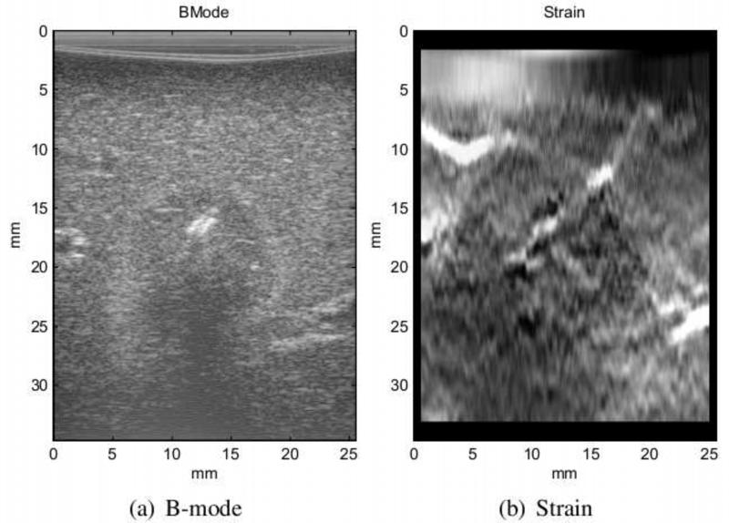
Ultrasound transducers are commonly tracked in modern ultrasound navigation/guidance systems. In this paper, we demonstrate the advantages of incorporating tracking information into ultrasound elastography for clinical applications. First, we address a common limitation of freehand palpation: speckle decorrelation due to out-of-plane probe motion. We show that by automatically selecting pairs of radio frequency (RF) frames with minimal lateral and out-of-plane motions combined with a fast and robust displacement estimation technique greatly improves in-vivo elastography results. We also use tracking information and image quality measure to fuse multiple images with similar strain that are taken roughly from the same location to obtain a high quality elastography image. Finally, we show that tracking information can be used to give the user partial control over the rate of compression. Our methods are tested on tissue mimicking phantom and experiments have been conducted on intra-operative data acquired during animal and human experiments involving liver ablation. Our results suggest that in challenging clinical conditions, our proposed method produces reliable strain images and eliminates the need for a manual search through the ultrasound data in order to find RF pairs suitable for elastography.

Introduction

Ultrasound elastography is enabled by applying a mechanical stimulus and estimating the disturbance created by this stimulus. Stimulus can be static mechanical load (Ophir et al., 1991), generated by external vibration (Parker et al., 1990), or through acoustic push signal (Berco et al., 2004). Estimation can be achieved by either tracking displacement or measuring the speed of propagating wave. A common flavor of this technology is quasi-static elastography in which the elastography image is generated by comparing the pre- and post-compression images to form a displacement map. The displacement can be then differentiated axially to find the strain map. When compression is applied to the tissue by hand via the ultrasound transducer, the elastography is referred to as “freehand elastography”. Many ultrasound systems are shipped with freehand elastography modules already installed. Note that this differs from freehand ultrasound in which the transducer is swept over the region of interest to create a volumetric (3D) image.

Physicians find elastography with freehand palpation natural as it resembles the centuries-old practice of examination by hand palpation. Moreover, ultrasound elastography does not necessarily require especial hardware or major alterations in the equipment and hence can be an integral part of any ultrasound system from high-end cart-based to pocket size systems.

Despite these advantages, freehand elastography introduces several challenges that have prevented the routine use of elastography in diagnoses and treatment of patients. This technique is highly qualitative and user-dependent. The best result is achieved when the examiner compresses and decompresses the tissue uniformly in the axial direction with the speed that produces proper strain rate (Ophir et al., 1999; Hall et al., 2003). Small lateral or out-of-plane motions can result in decorrelation which reduces signal-to-noise ratio (SNR) (Hall et al., 2003; Chandrasekhar et al., 2006). However, it is difficult to induce pure axial motion with freehand compression especially for slippery or oblique surfaces or for intra-operative imaging where the access to the tissue may be limited. The wide-spread clinical use of elastography could benefit from the development of elastography techniques that are less influenced by factors such as expertise of the user. It would also enable the longitudinal study of tumors where the strain images acquired during different time periods are compared.

Mechanical attachments designed to control the motion of probe can reduce role of the user. In (Hiltawsky et al., 2001), a mechanical compression applicator which applies uniform axial motion via compression plates was developed. The mechanical applicator reduced the amount of out-of-plane motion and consequently the dependency to the experience of the examiner. A 50% reduction in out-of-plane motion was reported in (Kadour and Noble, 2009) using an assistive hand-held device. In (Rivaz and Rohling, 2007), a low-frequency vibration was induced to the tissue while reaction forces were compensated. In a recent work, robotic palpation was studied for laparoscopic elastography (Billings et al., 2012). The main issues with mechanical solutions are that they require extra hardware, limit elastography to specific applications, make the probe bulky, and reduce its maneuverability.

Sophisticated algorithms have been developed that extend the search for displacement to lateral direction and tolerate certain amounts of decorrelation (Rivaz et al., 2008; Jiang and Hall, 2009; Pellot-Barakat et al., 2004). These algorithms can only partially address the problem by compensating for in-plane motions and enforcing smoothness constraints. However, they remain vulnerable to out-of-plane and large in-plane motions.

Another approach is to define a quality metric in order to evaluate the performance of strain images. Jiang et al. (2006) defined this metric as the multiplication of the Normalized Cross-Correlation (NCC) of the motion compensated RF fields (i.e. motion tracking accuracy) and the NCC of the motion compensated strain fields (i.e. consistency of strain images). This quality metric may be provided to the user as a feedback or used to combine multiple strain images. In (Jiang et al., 2007), they combined two strain images weighted by this metric to form a composite image. They also determined the gap between RF frames chosen for elastography by optimizing for this quality metric. Retrospectively processing the data, Lubinski et al. (1999) optimized the SNR. Using phantom studies, they showed that weighted averaging of displacement improves SNR. The weights were then adaptively selected for different frame step sizes.

Lindop et al. (2008) developed a framework in which the stream of strain images are normalized for the displacement estimates with a nonlinear function to compensate for uneven distribution of force and varying strain rates. The generated “pseudo-strain” images were then averaged over time on a “per-pixel basis” which depends on the precision of displacement estimation. The weights were also presented to the user as a feedback on the quality.

Normally the gap between frame pairs in elastography is fixed, and it is assumed that poor elastography results are detectable. Even when this gap is dynamically selected, the search range remains vary small. The other limitation of these approaches is that the strain has to be estimated prior to the calculation of the quality metric. With typical settings, the ultrasound frame rate can reach well above 30 Hz. For consecutive frames, an e cient implementation of these image-based metrics (probably with GPU acceleration) might accommodate this frame rate. However, the task will be extremely difficult when the aim is to evaluate all plausible combinations of frame pairs in a series of images.

It is common to localize the ultrasound transducer by attaching a position sensor to it. Some of the main applications of tracked ultrasound include volume reconstruction and extended field of view (Fenster et al., 2001), multi-modality registration (Gobbi et al., 1999; Foroughi et al., 2008), spatial compounding (Rohling et al., 1998), and navigation/guidance (Banovac et al., 2002; Sjolie et al., 2003). The growing interest in tracked ultrasound has led the emergence of ultrasound systems from companies such as “Ultrasonix”, “GE”, and “Siemens” which have electromagnetic (EM) sensors already embedded within their transducers.

The aim of this paper is to show that by tracking the ultrasound transducer, the information from the tracking device can be exploited to select pairs of RF frames for elastography which produce images with high SNR, contrast-to-noise ratio (CNR), and consistency. The frame selection happens before calculation of displacement and strain requiring negligible computational power. The selected frame pairs contain minimal lateral and out-of-plane motion and a predefined compression range with respect to each other. Based on tracking information, the strain images taken roughly from the same location are fused to obtain a high-quality elastography image. The method is validated using tissue mimicking phantom as well as intra-operative experiments on a porcine subject and on human patient data.

Methods

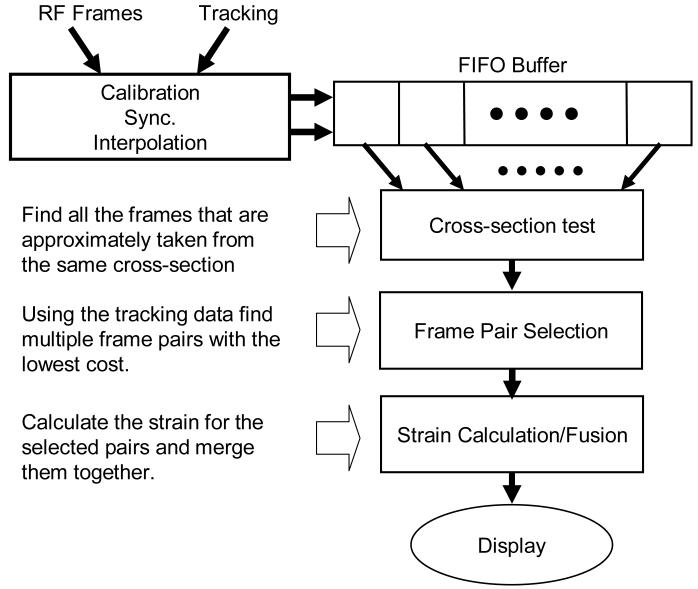
The block diagram of our algorithm summarizing the major steps are shown in Figure 1. As shown in this figure, the assumption is that a sequence of RF frames synchronized with tracking information is available to our algorithm in a buffer. For each RF frame in this buffer, a 6 DoF transformation is provided that determines the location of the RF frame at the time of its formation. Given this input, the task is to construct a high-quality 2D strain image.

Figure 1.

A block diagram illustrating the steps of the proposed method.

The cross-section test chooses a subset of these frames that are roughly taken from the same cross-section. The frame pair selection evaluates pairs of RF frames based on their tracking information and predicts which pairs generate acceptable strain images. The last step computes strain for all selected pairs and merges them together after compensating for the relative motion.

The core of our algorithm is a cost function that evaluates the motion between two frames and predicts the relative quality of the strain image without the need to compute the strain. Minimizing this cost function should minimize the overall speckle decorrelation between two frames. We start with a model for the speckle decorrelation, and use this model as a basis to define our cost function.

Decorrelation Model

The backscattered RF signal rf(t) is often modeled as the collective response of N scatterers randomly distributed within the resolution cell (Wagner et al., 1983) of the ultrasound (Wagner et al., 1983; Shankar, 2000):

$$rf\left(t\right)=\sum _{i=1}^N{a}_i\cos ({\omega }_{0}t+{\theta }_i),$$ (1)

where a_i and θ_i represent the random amplitude and the phase of the signal reflected by the ith scatterer. The distributions of a_i and θ_i are often assumed to be uniform. ω₀ is the mean frequency of excitation. Assuming fully developed speckle and Gaussian-shaped resolution cell, it is possible to show that the signal decorrelation, ρ(δ), caused by the displacement, δ, will have a Gaussian shape. Prager et al. (2003) proved the Gaussian shape of the correlation function for the “intensity” of the signal. A similar proof follows for the backscattered signal which gives:

$$\rho \left(\delta \right)=exp\left(\frac{-{\delta }^2}{4{\sigma }^2}\right).$$ (2)

σ is the standard deviation of the width of the resolution cell in the direction of the displacement. It should be noted that the decorrelation model is normally employed to estimate the displacement, whereas here, the correlation is estimated knowing the displacement. Extending Equation 2 to all three directions of displacement, a pseudo-correlation function, Crr, is defined as follows:

$$Crr(D_x,D_y,D_z)=exp(-K_x{D}_x^2-K_y{D}_y^2-K_z{D}_z^2),$$ (3)

where D_x, D_y, and D_z represent the displacement in out-of-plane, axial, and lateral directions respectively. K_x, K_y, and K_z determine the sensitivity to motion in their corresponding directions.

Distance Metric

Given the relative homogeneous transformation between two frames, Equation 3 can be used directly only when the relative rotation is ignored. However, even a small rotation may cause large decorrelation at the bottom of the image, and degrade the quality of the strain. At the same time, a component-wise metric is needed since the axial motion needs to be isolated as the desired type of motion. Suppose a = [a_x a_y a_z]^T is the axis-angle representation of the relative rotation, and t = [t_x t_y t_z]^T is the relative translation. Assuming a small rotation, the relative displacement of a point, P = [x y 0]^T, will be d = a × P + t. We then define the distance vector of two frames, D = [D_x D_y D_z]^T, as the RMS of the components of d for all the points in the region of interest (ROI):

$$\begin{array}{cc}\hfill D_x& =sqrt\left\{\frac{1}{y_{21}}{\int }_{y_1}^{y_2}{(-a_{z}x+t_x)}^{2}dy\right\},\hfill \\ \hfill D_y& =sqrt\left\{{\int }_{x_1}^{x_2}{(a_{z}x+t_y)}^{2}dx\right\},\hfill \\ \hfill D_z& =sqrt\left\{\frac{1}{y_{21}{x}_{21}}{\int }_{x_1}^{x_2}{\int }_{y_1}^{y_2}{(a_{x}y-a_{y}x+t_z)}^{2}dydx\right\},\hfill \end{array}$$ (4)

where sqrt{.} returns the root. The ROI is assumed to be rectangular and determined by x₁, x₂, y₁, and y₂. Symbols x₂₁ and y₂₁ are equal to x₂ - x₁ and y₂ - y₁ respectively. The vector D provides a measure of distance for each direction separately.

Frame Pair Selection

Given a sequence of RF frames, all possible combinations of frame pairs are evaluated using a slightly modified version of Crr. For M frames, there will be $\left(\begin{array}{c}\hfill M\hfill \\ \hfill 2\hfill \end{array}\right)=M(M-1)∕2$ pair combinations which provides more choices than consecutive frames. Since the pairs are directly compared, it su ces to minimize the negated exponent of Equation (3) in order to maximize Crr. Since axial motion is desired, the term for axial motion is also modified to penalize compressions that are higher or lower than the optimum compression value, t_opt. This forms a “cost function”, Cost, defined as follows:

$$Cost\left(D\right)=K_x{D}_x^2=K_x{D}_x^2+K_y\frac{{\mid D_y-t_{opt}\mid }^3}{D_y+c}+K_z{D}_z^2.$$ (5)

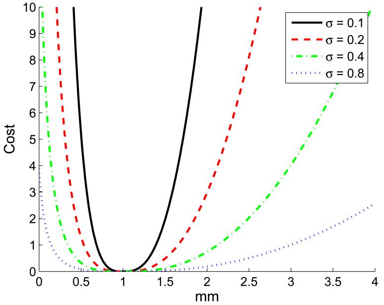
t_opt is determined based on the desired stain rate which is set by the user considering the amount of decorrelation that the elasticity estimation algorithm can handle. c is a small number that limits the cost of zero compression. With D_y much larger than t_opt, the second term of the cost function grows quadratically similar to that of lateral and out-of-plane motion. A D_y value close to zero also increases the cost preventing the selection of pairs with no axial motion. The sensitivity to the exact value of t_opt is adjusted by K_y (see Figure 2).

Figure 2.

The cost of axial motion for t_opt = 1 and K_y = (4σ²)⁻¹.

Using this function, multiple frame pairs with the lowest cost values are identified. In our implementation, a maximum of 8 frame pairs are selected to ensure an upper bound for the required processing time. A pair is rejected if the value of the cost function is above ln(2) (or equivalently when the pseudo-correlation drops to lower than 0.5).

Elastography and Fusion

To compute the displacement map for a pair of RF frames we have employed the “2D AM” technique (Rivaz et al., 2011) which is shown to be robust and fast. It computes a sub-pixel estimation of the motion field in both axial and lateral directions. The regularization terms makes it tolerant to outlier and noise. Furthermore, it can handle small internal motions induced by heartbeat or respiration. Since localization information is assumed to be available to us, we can automatically adjust the search range for the recovery of the motion field and increase the speed of displacement estimation.

Given the displacement map, the strain is computed by applying least squares fitting. The strain image is calculated for all selected pairs. The final image is found by merging the motion compensated strain images. Motion compensation is aimed to reduce the effect blurring caused by mixing strain images. Assume the selected frame pairs are $\left\{\right(I_1^1,I_1^2),(I_2^1,I_2^2),\dots ,(I_n^1,I_n^2\left)\right\}$ where n is the number of selected frame pairs resulting in the strain set {S₁, S₂, …, S_n}. $I_1^1$ is chosen as the reference frame and $I_2^1$ to $I_n^1$ are registered back to the reference frame to find their relative “global” compression and lateral motion. This registration is applied to a subset of RF intensities forming a grid, G. The tracking information is used to initialize the registration. G is comprised of a constant number (20) of rows and columns. This approach speeds up the optimization and makes it independent of the number of samples in the RF frames. For a pair of frames I¹ and I², the optimization function will be:

$$\arg \underset{a,b}{\max }\left\{\sum _{x,y\in G}\right\{I^1(x,y)\cdot I^2(x+a,by)+I^1(x-a,-by)\cdot I^2(x,y)\left\}\right\}.$$ (6)

The optimization variables a and b determine the lateral motion and axial compression respectively. The symmetric form of the objective function ensures that the optimization does not depend on the order of frames, and exchanging the frames only a ects the sign of the variables. The search spans of a and b are initialized from the tracking information. In the case of b, this range will be from zero to the value reported by the tracker since the actual observed compression might be less than that value. For both a and b, the search span is also extended in both sides with an assumed maximum error value for the tracker readings (0.2 mm). Note that the relative motion error is expected to be much lower than the absolute error.

The motion compensated strain images, ${\acute{S}}_i$, are constructed by applying the global deformation to the strain images (S_i). Since we are only interested in global motion, the registration is fast and unlikely to fail. These images are merged by weighted averaging in the pixel level to increase the SNR forming the output image, S_final:

$$S_{final}=\frac{{\sum }_{i=1}^n{w}_i\left(p\right)\cdot {\acute{S}}_i\left(p\right)}{{\sum }_{i=1}^n{w}_i\left(p\right)},w_i\left(p\right)={\rho }_i^{cost}\cdot {\rho }_i^{cc}\cdot {\rho }_i\left(p\right).$$ (7)

The weight factor, w_i(p), is found by multiplying three values, ${\rho }_i^{cost}$, ${\rho }_i^{cc}$, and ρ_i(p). ${\rho }_i^{cost}$ is the estimated correlation coefficient from the cost function of Equation 5 (${\rho }_i^{cost}=exp\{-Cos{t}_i\}$). ${\rho }_i^{cc}$ and ρ_i(p) represent the overall and pixel-level correlation coefficient of the RF frame pair after applying the estimated displacement. ${\rho }_i^{cost}$ reduces the bias toward lower compression created by the other two factors. This bias is due to the fact that in general pairs with lower compression yield higher correlation coefficient.

Whenever the overall correlation coefficient is low for a pair of images, the whole strain estimation cannot be trusted even if the pixel-level correlation for a specific area is high. The inclusion of ${\rho }_i^{cc}$ reduces the share of strain images with low overall correlation coefficient.

Cross-section Test

It is only meaningful to fuse images that are taken from roughly the same cross-section of tissue. The tracking data may be utilized to detect which frames are from one cross-section of the tissue with minimal lateral and out-of-plane motion. This is a step taken prior to the selection of frame pairs and provides the pool of frames from which the pairs are selected.

Since axial motion is not of interest in this case, K_y is set to zero in Equation 3 providing a “closeness measure.” Given a single frame, the closeness measure of this frame with respect to all other frames in the sequence is computed. These values are sorted in descending order, and the frames with closeness measure greater than 0.5 are chosen. A threshold on the maximum number of frames, M, is also applied which ensures that the number of frames from that cross-section is equal to or less than M. This process is carried out for all frames in the sequence and the set of frames with the largest sum of closeness measures is chosen.

One can also extract sets of frames from multiple cross-sections and generate a strain image for each cross-section. The availability of localization information means that a 3D strain volume could be automatically reconstructed.

Data Acquisition

System Specifications

Two different ultrasound systems were used to collect RF data. The data from phantom and pig experiments was collected using the SonixSP ultrasound system (Ultrasonix Medical Corp.) and the L12-5 transducer with central frequency of 10 MHz. The RF data was obtained via our interface software based on Ultrasonix research SDKs. This software controls RF acquisition and sends the data over a local network to a laptop computer where the RF frames are saved along with the tracking information. This is our preferred setup as it provides an excellent research interface and we have full control over the parameters of the ultrasound machine and the flow of the data.

In the case of patient experiments, the raw ultrasound data was obtained from an ACUSON Antares™ (Siemens Medical Solutions USA, Inc.), a high-end ultrasound system with an intra-operative ultrasound transducer (VF13-5SP) at center frequency of 8.89 MHz. The Axius Direct™ Ultrasound Research Interface was employed to enable RF acquisition and trigger the ultrasound system. For synchronization purposes, our software signaled both the ultrasound system and the external tracker the start of data collection. The duration of each sequence of RF frames was limited by the buffer size on the machine.

The localization information was gathered via a “medSAFE” electromagnetic (EM) tracker (Ascension Tech. Corp.) with model 180 sensors. The mid-range cubic transmitter supplied the magnetic field for all experiments except for the patient experiment where a “flatbed” transmitter was placed under the mattress of the surgical bed before the arrival of the patient. The data from the flatbed transmitter was filtered with a low pass filter to reduce the inherent jitter in the readings. The ultrasound transducer was calibrated using the standard cross-wire calibration (Prager et al., 1998).

Synchronization

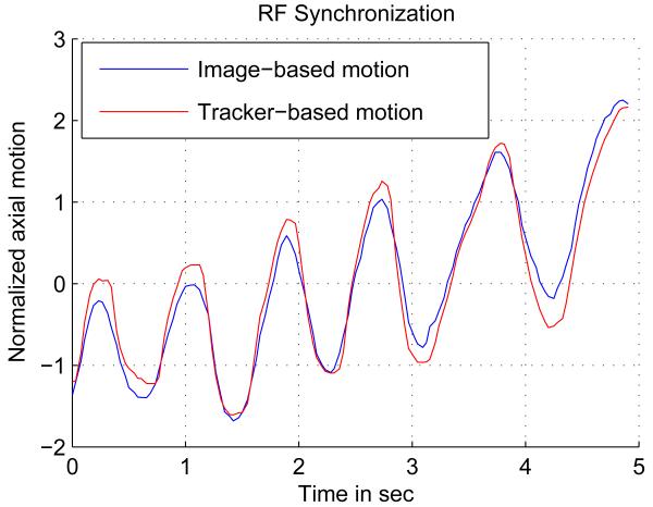
It is important for the success of this method to have the correspondence between the RF frames and the tracking data. Here, we rely on the timestamp of the tracker readings and the RF frames. The task of synchronization would be to find the constant delay between the two timestamps and compensate for that. This goal is achieved by exploiting the same freehand palpation used for elastography, which implies that no special procedure is required for synchronization. This also enables dynamic synchronization, where not only the constant delay between RF and tracker data is estimated as the data is collected, but also small jitters in delay are compensated. In this work, a constant delay is assumed since timestamps are available for the acquired data. To find this delay, the global axial compression is first recovered by correlating the first frame and the stretched version of the next frame. The same optimization procedure described by Equation 6 is employed for this purpose. The compression values are integrated over a period of time to get the compression with respect to the first frame in that period. The resulting curve is matched with the axial motion reading from the EM tracker using NCC. For both Ultrasonix and Antares machines, the tracker and RF data are synchronized using this technique. Figure 3 shows the two signals after the delay is compensated. To find the exact transformation for each RF frame, the tracking data interpolate. The translations and rotations are separately interpolated using “spline” interpolation for the translations and “spherical linear interpolation” (Slerp) (Shoemake, 1985) for the rotations.

Figure 3.

Axial palpation is used for synchronization.

Experiments

The performance of our algorithms is demonstrated with three sets of experiments: phantom, animal, and patient experiments. The phantom experiment provides a controlled environment for which the shape, location, and elasticity of the target is known. The pig experiment replicates the challenging environment of the operation room and surgery, but at the same time, control over the duration of the experiment and ultrasound system parameters is maintained. The gross pathology is also available as the pig is sacrificed at the end of the experiment. The patient experiment imposes a less controlled environment where the time for data collection is limited and minimal interference is introduced to the routine flow of the surgery.

Phantom experiment

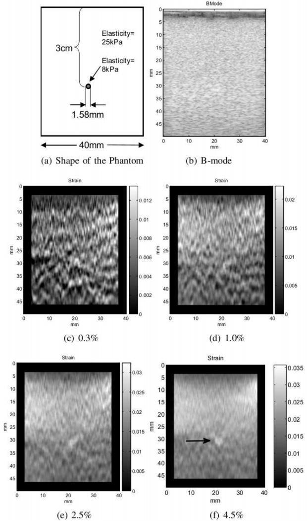
The data was taken from the CIRS (CIRS Inc. Norfolk, Virginia) elasticity phantom model 049A. Out-of-plane and lateral motion is less problematic for this experiment since the surface of the phantom is flat and there is more control over hand motion. However, low compression rate can a ect the quality of the strain image. Figure 4 shows four strain images with increasing compression rates taken from a 1.58 mm diameter lesion located at the depth of roughly 3 cm. The strain images are automatically generated from a “single” sequence of RF frames using our frame selection technique. This experiment demonstrates the capability of our frame selection in providing some level of control over the strain rate. It also shows that higher strain rates are more effective for scanning small lesions. This lesion is almost three times softer than the background and does not show up in the B-mode image (Figure 4(b)). In Figures 4(c-e), as the strain rate increases, enough SNR and contrast is achieved to make the lesion easily detectable. The diameter of the lesion in the image seems to be slightly larger than the original size. This could be due to smoothing constraints applied in the elastography algorithm and the least square fitting. The strain rates chosen by the user in Figures 4(c-f) are given in the figure caption. The algorithm tries to find the closest strain rate to these values. However, the strain rate may be lower than the selected value when not enough compression is applied by hand. In this case, the phantom was not compressed more than about 4% to prevent damaging it. The frame rate for RF data was about 30 frames per second which means for a slow palpation, a large gap between the frames (12 frames for 4(f)) was necessary to achieve the required strain.

Figure 4.

Four strain images with increasing compression rates are automatically generated from a single sequence. The structure of the phantom is shown in (a). The small lesion is not visible in the B-mode image displayed in (b). (c)-(f) shows the resulting strain image for the selected strain rate. The lesion is clearly visible in (f).

Animal experiment

Generating strain images intra-operatively is difficult since factors such as experimental time constraint, safety, and the introduction of surgical tools need to be taken into account. The access to the imaging area may be limited, and internal motions can be disruptive. In these conditions, axial hand motion mostly does not translate into simple up and down palpation. The force needs to be exerted with an oblique angle making it difficult to avoid lateral and out-of-plane motions. Moreover, the slippery surface of the tissue or the ultrasound gel applied to the surface of tissue causes the transducer to slide over the tissue. The aim of this experiment is to show the benefit of the proposed technique for intra-operative imaging.

Our protocol for animal experiment was approved by the Johns Hopkins University Institutional Care and Animal Use Committee (IACUC). For this experiment, the cubic electromagnetic transmitter was secured on the bed side prior to the arrival of the pig. The pig was then prepared for the surgery, and the liver was exposed for ablation. Next, the ablation needle was inserted inside the liver under ultrasound guidance. The liver was then ablated to create an ablation zone of about 2 to 3 cm. After the ablation, the needle was removed and a sequence of tracked RF data was collected from the ablated region. The data collection was carried out a few minutes after the ablation to allow for the dispersion of the bubbles caused by the ablation procedure. The placement of the probe and the direction of the needle were marked on the surface of the liver by two small burns on both sides of the transducer and a third arrow-shaped burn mark. Three zones were ablated creating three hard lesions (a fourth lesion was also ablated for a separate experiment). Finally, the pig was sacrificed and the liver was harvested. Guided by the burn marks, the liver was cut on approximately the same plane as the ultrasound data was gathered.

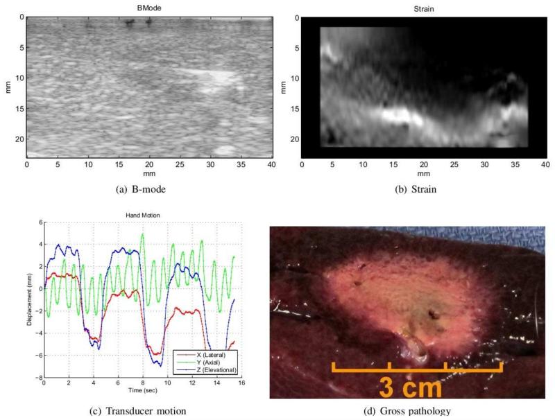
Figure 5 shows the B-mode, strain, translational motion from tracking, and the gross pathology of the ablated zone. The core of the ablation appears as a slightly hypoechoic region in the B-mode image. Compared to the whole ablated region, this core is smaller and contains the dehydrated tissue for which the acoustic properties are mildly modified. The needle imprint is also visible as a hyperechoic line inside the ablation. The strain image shown in Figure 5(b) is the output of our algorithm. The ablation is harder than the surrounding tissue and appears darker in the strain image. It is larger than the hypoechoic region in the B-mode image, and its size matches the size of ablation from gross pathology (Figure 5(d)).

Figure 5.

The figure shows in-vivo ablation experiment on pig liver. The B-mode image (a) only shows the core of ablation composed of dehydrated tissue. The strain in (b) is generated by our method and depicts the ablated zone in dark. The size of hard lesion in strain image matches gross pathology shown in (d). The relative translational motion of the frames with respect to the first frame is presented in (c). The breathing motion is captured in the lateral and elevational components of the tracking data.

The graph in Figure 5(c) displays the translational motion of the ultrasound plane with respect to the first frame in the sequence. The effect of respiration is captured in the lateral and elevational components of the tracking information as a periodic cycle. In this case, the breathing pushed the liver which in turn caused the motion of the transducer placed on the top of it. Only the frames from the resting portion of the breathing cycle are suitable for computation of strain as the breathing motion may cause the transducer to slide over the tissue. The presented algorithm can automatically compute the strain from only the resting phase of respiration as long as the breathing cycle is captured in the tracking data. This observation was possible in the animal experiment since the data collection system permits long sequences of images containing several breathing cycles to be obtained.

Patient experiment

The protocol for patient experiment was approved by the Johns Hopkins institutional review board (IRB), and informed consent was acquired. In this experiment, raw ultrasound data was obtained from a cancer patient undergoing multiple liver wedge resections and radiofrequency ablations of metastatic lesions. In order to introduce minimal deviation to the normal flow of the surgery, only one lesion was imaged before and after ablation. The ultrasound data acquisition was quick and added only a few minutes to the total length of the surgery.

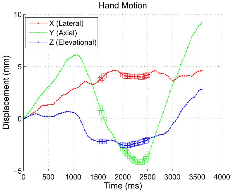
To collect the ultrasound data, the surgeon had to slide the ultrasound probe inside the abdominal cavity through the surgical incision making out-of-plane motion and probe sliding nearly unavoidable. This can be seen in Figure 6 which shows the translational component of the hand motion of the surgeon during data collection. The frames selected by the “crosssection test” are marked by small squares on the top of the motion curve. From Figure 6 it could be noted that these frames have lower lateral and elevational (out-of-plane) motion with respect to each other.

Figure 6.

The translational component of the hand motion of the surgeon w.r.t. the first frame in the sequence.

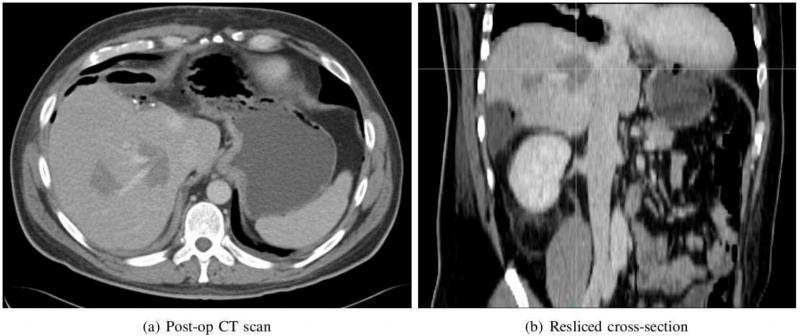
The pre- and post-operation CT scans of the patient were taken as a routine part of the operation. In the pre-operative CT scan, the contrast between the tumor and background was very low, and an accurate comparison between CT and ultrasound could not be established. The post-operation CT scan of the patient is presented in Figure 7 where (a) contains the ablated region and (b) is the resliced cross-section that roughly matches the plane of ultrasound imaging. The vascular structure in the CT scan taken in venous phase appears brighter, and the ablated region is darker compared to the normal liver tissue. To compare strain and CT, the plane in CT volume corresponding to the strain should be found. This could be achieved relying on anatomical features as proposed in Clements et al. (2008). In this work, we rely on three clues to reslice the CT volume. The first is the shape of the ablation which is extended toward the direction of the needle. From the shape, we were able to approximate the position of the needle in the CT scan. We also collected a series of tracked ultrasound images containing the track of the needle. The position of the needle in CT and ultrasound was then matched. The elastography data was obtained from an almost perpendicular plane to the plane of the needle avoiding the distortion from the needle. Assuming minimal motion during ultrasound data acquisition, the spatial relation of the image with the needle and the elastography image could be determined. Although the rotation of the slice could not be determined with this method, the size of the ablated zone is measurable. In Figure 7(a), there are two ablated regions visible out of which only the ablation on the right side was imaged. The pixel spacing (x and y directions) is 0.7 mm and the slice thickness is 3 mm. The diameter of the ablated zone is about 19 mm.

Figure 7.

Post-operation CT scan of the ablated region. The plane of resliced cross-section roughly matches the plane of ultrasound image.

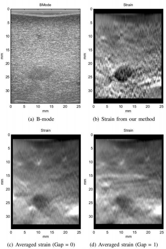
The elastography results of the tumor before and after ablation are depicted in Figures 8 and 9. Prior to ablation, the tumor appears as a hypoechoic region in the B-mode ultrasound image (Figure 8(a)). Since the tumor is harder than the surrounding tissue, it is darker in the strain image. The border of the tumor and its shape are better distinguishable in the elastography image. The B-mode and strain images of the tumor after ablation shown in Figure 9 have similar characteristics to those of the animal experiment. A slightly hypoechoic core is visible in the B-mode image which is created by the dehydrated tissue similar to the animal experiment. This region is smaller than what is detectable in the CT scan. The size of the ablation in the elastography image is approximately 17 mm which is closer to the size of the ablation in Figure 7(b).

Figure 8.

The B-mode ultrasound and strain image of the tumor prior to ablation.

Figure 9.

The B-mode and strain image of the tumor after the ablation.

Quantitative Results

SNR and CNR are the most common measures used for quantifying the quality of the strain image. The SNR and CNR values are computed from (Chaturvedi et al., 1998):

$$\mathrm{CNR}=\sqrt{\frac{2{({\stackrel{‒}{s}}_b-{\stackrel{‒}{s}}_t)}^2}{{\sigma }_b^2+{\sigma }_t^2}},\mathrm{SNR}=\frac{\stackrel{‒}{s}}{\sigma },$$ (8)

where s̄ and σ denote the mean and standard deviation of intensities. The t or b subscripts mean that the computation is only for the target or the background region, respectively.

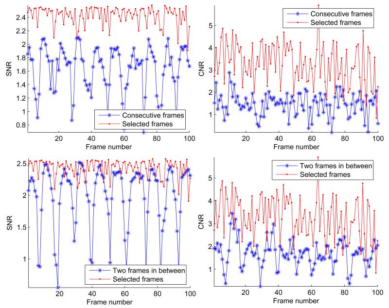
Figure 10 shows the SNR and CNR for the CIRS phantom with a hard inclusion that is twice sti er than the background. The results are presented for strain images generated from the automatically selected frames, consecutive frames, and a constant gap of two frames. Our method consistently selects frame pairs which produce strain images with higher SNR and CNR values. The drop in SNR is more prominent for consecutive frames where there is not enough compression between the frames. Increasing the gap improves the SNR and CNR for some frames while reduces these values for other frames due to decorrelation (see the bottom row of Figure 10). The periodic behavior of SNR for the constant gap roughly matches cycles of the axial motion by hand. The reason is that the speed of hand motion is variable and the step size is not adjusted accordingly.

Figure 10.

The strain images from the top 100 frame pairs selected by our algorithm vs. consecutive frames. In the top row, the step size is zero whereas in the bottom row the step size is two. In both cases, the strain images from the automatically selected frames maintain higher SNR and CNR values. Although the mean CNR and SNR slightly rises when the constant gap between the frames is increased, the variations of these values surges.

Averaging a large number of strain images increases the SNR of the signal as shown in (Lubinski et al., 1999). However, it blurs the strain image as demonstrated in Figures 8(c) and 8(d). The blurring is mainly due to the displacement of the tumor in the strain sequence which includes out-of-plane motion. Table 1 shows the surge in SNR and CNR as a result of averaging especially for successive frames for the pre-ablated tumor in our patient experiment. These values are still less than those of our method although the number of frame pairs used is ten-fold larger. At the same time, the quality of the final image is severely degraded due to the displacement of the tumor during data collection.

Table 1.

The comparison of averaging strain images from consecutive frames with fixed gap size and frame selection.

	Gap between frames (50 frame pairs)				Frame Selection (5 frame pairs)
	Zero	One	Two	Three
Avg. CNR	0.78(0.32)	0.94(0.43)	1.04(0.42)	1.02(0.51)	1.57(0.37)
Avg. SNR	1.35(0.42)	1.20(0.56)	1.16(0.63)	1.11(0.70)	1.96(0.10)
CNR of Avg.	1.62	1.09	1	0.12	1.97
SNR of Avg.	2.2	1.88	1.44	1.13	2.36

In Table 2, our frame selection technique is compared to the selection of consecutive frames. The SNR, correlation coefficient, and strain consistency of the selected frames are being compared for all our experiments. The number of frames used in both methods are fixed (five frame pairs). For consecutive frame selection the average over the whole sequence (100 frames) is presented. The standard deviation of each value is shown in parenthesis.

Table 2.

Comparison of the performance of selecting consecutive frames with our frame selection method. “FS” stands for our frame selection method. The mean and standard deviation (in parenthesis) for each case is presented. The first column shows the experiment numbers which correspond to the following experiments respectively: Phantom, Pig Liver lesion 1, Pig Liver lesion 2, Pig Liver lesion 3, Pre-ablated tumor in patient, Post-ablated tumor in patient.

	Consistency		Correlation Coef.		SNR
	FS	Consec.	FS	Consec.	FS	Consec.	Final FS
1	0.75(0.11)	0.21(0.15)	0.92(0.04)	0.91(0.09)	1.82(0.21)	0.40(0.56)	2.08
2	0.93(0.05)	0.56(0.25)	0.92(0.01)	0.94(0.02)	0.84(0.21)	0.85(0.44)	1.09
3	0.85(0.08)	0.57(0.26)	0.84(0.04)	0.86(0.04)	0.65(0.14)	0.52(0.24)	0.94
4	0.72(0.14)	0.56(0.21)	0.86(0.05)	0.92(0.04)	0.94(0.20)	0.78(0.33)	1.45
5	0.80(0.15)	0.54(0.18)	0.98(0.01)	0.99(0.00)	1.96(0.10)	1.35(0.42)	2.44
6	0.83(0.10)	0.49(0.20)	0.98(0.01)	0.99(0.01)	1.70(0.10)	1.13(0.45)	1.91

The correlation coefficient is the same as ${\rho }_i^{cc}$ in Equation 7. The two methods produce comparable correlation coefficient, but for consecutive frames this number is slightly higher. Selecting consecutive frames normally yields the highest correlation coefficient. This does not translate into higher quality of elastography. The reverse is however true. If the correlation coefficient is low, the output image is not reliable. In all cases, the value of correlation coefficient remained above 0.80 which means that the displacement estimation did not fail.

Consistency among strain images has been suggested as a good measure for the quality of the images. Jiang et al. (2006) defined a performance descriptor based on consistency of two consecutive stain images. They showed that this descriptor correlates with the CNR and human ranking score. The consistency is defined as the NCC of the two strain images. Here, the consistency of more than two images is examined. For this purpose, the NCC for all possible pairs of strain images is computed. The average and standard deviation of this value is reported in Table 2. The range of this value is from zero to one. For both consecutive frames and selected pairs, the number of strain images is set to 5 resulting in 10 possible combinations. In all cases of our experiments, the average consistency is significantly better for the frame pairs selected using the tracking information while the standard deviation is lower.

Discussion

Choosing the right frame pairs is essential for the success of elastography in clinical conditions. Frame selection using tracking reduces the dependency of elastography to the quality of hand motion and provides control over the rate of compression. It is an effective tool especially since the rate of ultrasound data is very high. The computational cost of evaluating frame transformations is practically ignorable compared to the cost of strain estimation which makes it possible to analyze hundreds of frame pairs prior to strain calculation. The combination of this technique with strain motion compensation and the pixel-wise image fusion significantly elevates the quality and reliability of elastography.

Although an additional tracking device is required for this method, localization data is already available to many ultrasound navigation systems. The arrival of new ultrasound systems that embed the localizing sensor within the probe suggests a rising trend for such systems. We believe that elastography can become an essential element of these systems to aid the diagnoses, monitoring, or targeting in clinical applications. In our experiments, the source of tracking was an EM tracker. Nonetheless, other types of tracking devices such as optical trackers or accelerometers could also be employed for this purpose.

We showed that blindly averaging strain images could introduce significant blurring. Much better results can be achieved with a smaller number of images that are carefully selected using the tracking information. For the last step of this technique, a similar approach to what has been suggested in (Jiang et al., 2007) or (Lindop et al., 2008) could also be adopted to further refine the results of elastography.

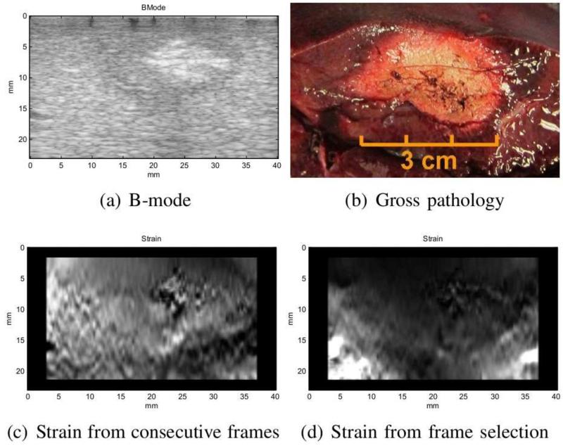
The frame selection method generally produces results with higher SNR. Both the average SNR of the selected frames and the SNR of the fused image are reported in Table 2. As expected, the combined SNR value is higher than that of individual images. Although the SNR value seems to be a better indicator of the quality of the image, there are some cases where this value might be misleading. Specifically for the second pig ablation, the consecutive frames produced better SNR. However, this is due to the fact that the image in that case contains a large hard lesion which a ects the mean of the strain and therefore, reduces SNR (Figure 11). As shown in Figure 11(c), the noise in the individual strain images has caused the lesion appear softer than its actual sti ness in the averaged image. This is also partly the result of the regularization term in displacement estimation when the compression is very low. In this case, the relatively higher value of SNR (1.14) is only the result of the increase in the mean value of the strain. In frame selection method, low compression and unwanted motions are avoided resulting in an image that is in agreement with gross pathology. The 3 cm size of ablation in Figure 11(d) matches the measurement from gross pathology (Figure 11(b)).

Figure 11.

The results of second ablated region in pig experiment. The strain from consecutive frames has relatively high SNR but very low consistency.

Consistency among frames seems to be the best indicator of failure. With multiple strain images from one cross-section available, this indicator could be employed to detect failed images and eliminate them in the final step. However, this will introduce additional computational cost to the system.

Our data acquisition interface, developed in C++, undertakes the tasks of connecting to the ultrasound machine and tracking device, synchronizing the acquisition, and recording the data. Currently, our implementation is in MATLAB and all the processing is preformed off-line. However, there are no computational limitations for processing the data in real-time as the data is being collected. The “2D AM” method (Rivaz et al., 2011) appears to be both fast and robust, and the image fusion could be implemented in real-time as it only involves 2D image mapping and weighted averaging.

Conclusion

In this paper, we presented a method to incorporate the information from a tracking device in elastography to tackle the challenges of clinical applications. In our experiments, the consistency and the SNR of strain images is increased by 67% and 97% respectively. This is a pilot study aimed to demonstrate the potential of this approach to reliably produce high quality strain images. Further clinical trials are necessary to fully evaluate the diagnostic impact of our frame selection. This system could particularly be effective for the intra-operative procedures where traditionally manual search through the frames is needed after data collection in order to find the pair that generates an acceptable image. In conjunction with the incorporation of tracking, our method benefits from e cacious displacement estimation and image fusion techniques making it resilient to failure.

There are numerous possibilities to improve this elastography system. In the presence of tracking data, an immediate improvement could be the addition of hand motion feedback to the user. This will involve developing easy-to-understand interfaces which will provide real-time feedback during hand palpation. 3D strain imaging from the 2D images will also be a natural extension to this system. This will be similar to the volume reconstruction from 2D B-mode images with the exception that the localization information will be used not only for placing the strain images inside the volume, but also for frame selection. Finally, the full integration of this system in a clinical platform will allow for clinical trials for specific applications.

References

- Banovac F, Glossop N, Lindisch D, Tanaka D, Levy E, Cleary K. Medical Image Computing and Computer-Assisted Intervention. Vol. 2488. Springer; Berlin/Heidelberg: 2002. Liver tumor biopsy in a respiring phantom with the assistance of a novel electromagnetic navigation device; pp. 200–207. [Google Scholar]
- Berco J, Tanter M, Fink M. Supersonic shear imaging: a new technique for soft tissue elasticity mapping. IEEE Transactions on Ultrasonics, Ferroelectrics and Frequency Control. 2004;514:396–409. doi: 10.1109/tuffc.2004.1295425. [DOI] [PubMed] [Google Scholar]
- Billings S, Deshmukh N, Kang HJ, Taylor RH, Boctor E. Medical Imaging 2012: Image-Guided Procedures, Robotic Interventions, and Modeling. Proceedings of SPIE. 2012. System for robot-assisted real-time laparoscopic ultrasound elastography. In Press. [Google Scholar]
- Chandrasekhar R, Ophir J, Krouskop T, Ophir K. Elastographic image quality vs. tissue motion in vivo. Ultrasound in Medicine & Biology. 2006;326:847–855. doi: 10.1016/j.ultrasmedbio.2006.02.1407. [DOI] [PubMed] [Google Scholar]
- Chaturvedi P, Insana MF, Hall TJ. Testing the limitations of 2-D companding for strain imaging using phantoms. IEEE Transactions on Ultrasonics, Ferroelectrics and Frequency Control. 1998;45:1022–1031. doi: 10.1109/58.710585. [DOI] [PubMed] [Google Scholar]
- Clements LW, Chapman WC, Dawant BM, Galloway RL, Miga MI. Robust surface registration using salient anatomical features for image-guided liver surgery: Algorithm and validation. Medical Physics. 2008;356:2528–2540. doi: 10.1118/1.2911920. [DOI] [PMC free article] [PubMed] [Google Scholar]
- Fenster A, Downey DB, Cardinal HN. Three-dimensional ultrasound imaging. Physics in Medicine and Biology. 2001;465:R67–R99. doi: 10.1088/0031-9155/46/5/201. [DOI] [PubMed] [Google Scholar]
- Foroughi P, Song D, Chintalapani G, Taylor RH, Fichtinger G. Localization of pelvic anatomical coordinate system using US/atlas registration for total hip replacement; Proceedings of the 11th International Conference on Medical Image Computing and Computer-Assisted Intervention, Part II; 2008; Springer-Verlag; pp. 871–879. [DOI] [PubMed] [Google Scholar]
- Gobbi DG, Comeau RM, Peters TM. Proceedings of the Second International Conference on Medical Image Computing and Computer-Assisted Intervention; Ultrasound probe tracking for real-time ultrasound/MRI overlay and visualization of brain shift; 1999; Springer-Verlag; pp. 920–927. [Google Scholar]
- Hall TJ, Zhu Y, Spalding CS. In vivo real-time freehand palpation imaging. Ultrasound in Medicine & Biology. 2003;293:427–435. doi: 10.1016/s0301-5629(02)00733-0. [DOI] [PubMed] [Google Scholar]
- Hiltawsky KM, Krger M, Starke C, Heuser L, Ermert H, Jensen A. Freehand ultrasound elastography of breast lesions: clinical results. Ultrasound in Medicine & Biology. 2001;2711:1461–1469. doi: 10.1016/s0301-5629(01)00434-3. [DOI] [PubMed] [Google Scholar]
- Jiang J, Hall T, Sommer A. A novel performance descriptor for ultrasonic strain imaging: a preliminary study. Ultrasonics, Ferroelectrics and Frequency Control, IEEE Transactions on. 2006;536:1088–1102. doi: 10.1109/tuffc.2006.1642508. [DOI] [PMC free article] [PubMed] [Google Scholar]
- Jiang J, Hall TJ. A generalized speckle tracking algorithm for ultrasonic strain imaging using dynamic programming. Ultrasound in Medicine & Biology. 2009;3511:1863–1879. doi: 10.1016/j.ultrasmedbio.2009.05.016. [DOI] [PMC free article] [PubMed] [Google Scholar]
- Jiang J, Hall TJ, Sommer AM. A novel image formation method for ultrasonic strain imaging. Ultrasound in Medicine & Biology. 2007;334:643–652. doi: 10.1016/j.ultrasmedbio.2006.11.005. [DOI] [PMC free article] [PubMed] [Google Scholar]
- Kadour M, Noble J. Assisted-freehand ultrasound elasticity imaging. Ultrasonics, Ferroelectrics and Frequency Control, IEEE Transactions on. 2009;561:36–43. doi: 10.1109/TUFFC.2009.1003. [DOI] [PubMed] [Google Scholar]
- Lindop JE, Treece GM, Gee AH, Prager RW. An intelligent interface for freehand strain imaging. Ultrasound Med Biol. 2008;34:1117–1128. doi: 10.1016/j.ultrasmedbio.2007.12.012. [DOI] [PubMed] [Google Scholar]
- Lubinski M, Emelianov S, O’Donnell M. Adaptive strain estimation using retrospective processing [medical us elasticity imaging] Ultrasonics, Ferroelectrics and Frequency Control, IEEE Transactions on. 1999;461:97–107. doi: 10.1109/58.741428. [DOI] [PubMed] [Google Scholar]
- Ophir J, Alam S, Garra B, Kallel F, Konofagou E, Krouskop T, Varghese T. Elastography: ultrasonic estimation and imaging of the elastic properties of tissues. Annu. Rev. Biomed. Eng. 1999;213:203–233. doi: 10.1243/0954411991534933. [DOI] [PubMed] [Google Scholar]
- Ophir J, Cspedes I, Ponnekanti H, Yazdi Y, Li X. Elastography: a quantitative method for imaging the elasticity of biological tissues. Ultrasonic imaging. 1991;13:111–134. doi: 10.1177/016173469101300201. [DOI] [PubMed] [Google Scholar]
- Parker K, Huang S, Musulin R, Lerner R. Tissue response to mechanical vibrations for sonoelasticity imaging. Ultrasound in Medicine & Biology. 1990;163:241–246. doi: 10.1016/0301-5629(90)90003-u. [DOI] [PubMed] [Google Scholar]
- Pellot-Barakat C, Frouin F, Insana M, Herment A. Ultrasound elastography based on multiscale estimations of regularized displacement fields. Medical Imaging, IEEE Transactions on. 2004;232:153–163. doi: 10.1109/TMI.2003.822825. [DOI] [PMC free article] [PubMed] [Google Scholar]
- Prager R, Gee A, Treece G, Cash C, Berman L. Sensorless freehand 3-d ultrasound using regression of the echo intensity. Ultrasound Med. Biol. 2003;29:437–446. doi: 10.1016/s0301-5629(02)00703-2. [DOI] [PubMed] [Google Scholar]
- Prager RW, Rohling RN, Gee AH, Berman L. Rapid calibration for 3-D freehand ultrasound. Ultrasound in Medicine and Biology. 1998;246:855–869. doi: 10.1016/s0301-5629(98)00044-1. [DOI] [PubMed] [Google Scholar]
- Rivaz H, Boctor E, Choti M, Hager G. Real-time regularized ultrasound elastography. Medical Imaging, IEEE Transactions on. 2011;304:928–945. doi: 10.1109/TMI.2010.2091966. [DOI] [PubMed] [Google Scholar]
- Rivaz H, Boctor E, Foroughi P, Zellars R, Fichtinger G, Hager G. Ultrasound elastography: a dynamic programming approach. IEEE Transaction in Medical Imaging. 2008;27:1373–1377. doi: 10.1109/TMI.2008.917243. [DOI] [PubMed] [Google Scholar]
- Rivaz H, Rohling R. An active dynamic vibration absorber for a hand-held vibro-elastography probe. Journal of Vibration and Acoustics. 2007;1291:101–112. [Google Scholar]
- Rohling RN, Gee AH, Berman L. Automatic registration of 3-D ultrasound images. Ultrasound Med. Biol. 1998;246:841–854. doi: 10.1016/s0301-5629(97)00210-x. [DOI] [PubMed] [Google Scholar]
- Shankar P. A general statistical model for ultrasonic backscattering from tissues. IEEE Trans Ultrason Ferroelectr Freq Control. 2000;473:727–736. doi: 10.1109/58.842062. [DOI] [PubMed] [Google Scholar]
- Shoemake K. Animating rotation with quaternion curves. Computer Graphics (Proc. of SIGGRAPH) 1985:245–254. [Google Scholar]
- Sjolie E, Lango T, Ystgaard B, Tangen G, Nagelhus Hernes T, Marvik R. 3D ultrasound-based navigation for radiofrequency thermal ablation in the treatment of liver malignancies. Surgical Endoscopy. 2003;17:933–938. doi: 10.1007/s00464-002-9116-z. [DOI] [PubMed] [Google Scholar]
- Wagner R, Smith S, Sandrik J, Lopez H. Statistics of Speckle in Ultrasound B-Scans. IEEE Trans. Sonics and Ultrasonics. 1983;173:251–268. [Google Scholar]