

Abstract
Ultrasonic displacement estimates have numerous clinical uses including blood-flow, elastography, therapeutic guidance and ARFI imaging. These clinical tasks could be improved with better ultrasonic displacement estimates. Traditional ultrasonic displacement estimates are limited by the Cramer-Rao lower bound (CRLB). The CRLB can be surpassed using biased estimates. In this paper a framework for biased estimation using Bayes’ theorem is described.
The Bayesian displacement estimation method is tested against simulations of several common types of motion: bulk, step, compression, and acoustic radiation force induced motion. Bayesian estimation is also applied to in vivo acoustic radiation force imaging of cardiac ablation lesions. The Bayesian estimators are compared to the unbiased estimator, normalized cross-correlation.
As an example, the peak displacement of the simulated acoustic radiation force response is reported since this position results in the noisiest estimates. Estimates were made with a 1.5 λ kernel and 20 dB SNR on 100 data realizations. Estimates using normalized cross-correlation and the Bayes’ estimator had mean-square errors of 17 and 7.6 μm2, respectively, and contextualized by the true displacement magnitude, 10.9 μm. Biases for normalized cross-correlation and the Bayes’ estimator are −.12 and −.28 μm, respectively. In vivo results show qualitative improvements. The results show that with small amounts of additional information significantly improved performance can be realized.
I. INTRODUCTION
To the end of creating displacements estimators that bypass fundamental limits on common estimators, such as normalized cross-correlation, a perturbation to the traditional likelihood function was proposed in the accompanying paper and shown to be more discriminative in the sense of appropriately concentrating probability distributions around the true displacement [1]. In addition to presenting a modified likelihood function, biased estimators were introduced in a qualitative manner. In this paper biased estimators are implemented, and it is shown that with relatively small amounts of additional information it is possible to surpass the performance limit described by the Cramer-Rao lower bound.
The Cramer-Rao lower bound is a general measure of information content that describes the minimum obtainable estimation error variance when using an unbiased estimator [2]. A Cramer-Rao lower bound for displacement estimation related tasks has been derived in the ultrasound literature [3]–[7], but the derivation by Walker and Trahey [6] seems to be favored (probably because of broad applicability) and is
| (1) |
where f0 is the pulse center frequency, B is the pulse bandwidth, T is the kernel size, ρ is the normalized correlation between signals, and SNR is signal to noise ratio.
The Cramer-Rao lower bound limited estimator—usually referred to as the minimum variance unbiased estimator (MVUE)—is unique because the algorithmically induced bias is zero, which can be useful. The utility of the unbiased nature is seen in situations where many independent measurements can be acquired. In this case, the mean of all the estimates will converge towards the true measurement. However, in most clinical scenarios it is not possible to obtain multiple measurements. In in vivo scenarios where only a single estimate can be acquired the bias error is often over emphasized as a noise mechanism. This is because for a single estimate it is not possible to distinguish between different orthogonal error components [8]. By considering both noise mechanisms—bias and variance—a better estimator can often be realized.
Bias and variance of an estimator’s error are defined as
| (2) |
| (3) |
where τ0 describes the true estimate and describes the estimated time shift (i.e. displacement) between two signals. Both noise mechanisms can be appropriately combined in the form of the mean square error (MSE), which is
| (4) |
In many cases allowing a small amount of bias into an estimator can lead to a drastic reduction in the estimation variance creating an overall lower MSE. Fig. 1 shows an example of two different hypothetical biased estimators and how they might compare to an unbiased estimator that is Cramer-Rao lower bound limited.
Fig. 1.
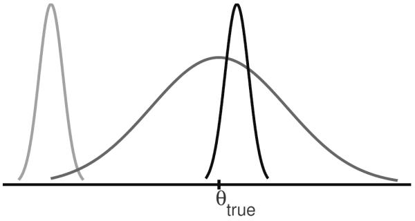
Three distributions describing the error of different hypothetical estimators are shown. The broad distribution can be equated to a MVUE, which would be described by the Cramer-Rao lower bound. The other two estimators have a significantly smaller variance. The estimator with the small bias to the right of θtrue is attractive, while the other biased estimator is clearly not.
In the ultrasound literature there have been no descriptions of biased displacement estimators that produce estimates with a lower MSE than would be produced by a minimum variance unbiased estimator. Several groups have produced estimator schemes where the displacement search region is shifted and reduced in size based on displacements measured at adjacent positions [9]–[11], but because of the way these algorithms are implemented they only achieve improvements in computational efficiency and in reduction of peak-hopping artifacts rather than an improvement in the actual MSE. (This type of approach will be shown to be a specific realization of the methods developed herein.)
In the rest of this paper biased displacement estimates with mean-square error surpassing the limit expressed by the Cramer-Rao lower bound will be demonstrated for several different types of motion.
II. METHODS
A. Overview
It is difficult to create estimators with improved MSE characteristics relative to the MVUE using classical methods [2]. The usual alternative is to use Bayes’ theorem, which is a simple equation describing the appropriate method for combining the current data with previous knowledge about the parameter(s) to be estimated [8]. Bayes’ theorem will be used for ultrasound displacement estimation to appropriately combine information from a local similarity function and prior information about the displacement to provide a better estimate for the current displacement estimate. To this end, Bayes’ theorem is expressed as
| (5) |
where x is the data, τ0 is the displacement, and m indexes axial depth. The term pm(x | τ0) denotes the likelihood function, pm(τ0) is the prior probability density function (PDF), and pm(τ0 | x) is the posterior PDF. The likelihood function is the means by which data is incorporated into the estimate. An appropriate and implementable likelihood function has been demonstrated in the companion paper to this one [1] and is
| (6) |
where sm1 and sm2 are the RF A-lines from which motion will be estimated, α is an application specific scaling term, Δ is the sampling period, and M is the length of the data record (i.e. kernel length). The quality metric for this function is normalized cross-correlation and the SNR is calculated as
| (7) |
The prior distribution expresses previous knowledge of the displacement and is a PDF. Example uses of prior PDFs would be to use the knowledge of an ARF dynamic response through depth to allow adjacent spatial locations to appropriately influence the current estimate, or similarly, in the case of blood flow estimation one could use fluid dynamics to influence adjacent spatial locations [12]. The posterior distribution is also a PDF and represents the final state of knowledge of the parameter(s) to be estimated after combining the new and old information. Displacement estimates at a given depth position will be made from the posterior distribution.
Two simple methods for obtaining prior PDFs of the displacement estimate will be described. Accompanying the description of prior PDFs will be a description of appropriate estimators for resolving the final posterior distribution into estimates of displacements.
B. Prior Probabilities
Methods for computing prior probabilities for ultrasound displacements is an open-ended, flexible problem with many solutions. Two solutions for computing prior probabilities will be developed in this section. The intention of the proposed methods will not be to present a broadly generalizable optimal prior PDF but rather to demonstrate the promise of biased estimators and the small amount of additional information needed to surpass the CRLB. The simplest, least-informative prior for ultrasound displacement estimation is a uniform PDF with an extent equivalent to the search region. This prior is described as
| (8) |
where τα and τβ denote the limits of the search region. The mean and variance of the uniform prior can be static for all displacement estimates in the field, or the uniform PDFs can be dynamic based on other information such as spatially adjacent displacements [9]–[11]. For the evaluation here the uniform PDF is static with depth.
The second prior scheme that will be explored is more dynamic than the uniform PDF proposed above. In this scheme the posterior distribution at the previous depth will be considered a good estimate for the prior distribution at the current depth. When the previous posterior gets too narrow based on the posterior’s standard deviation the prior will revert to a normal distribution with mean equal to the previous estimate and a standard deviation equal to a defined minimum standard deviation. That is,
| (9) |
where is the estimate at the previous depth and the variance is a pre-defined σmin.
In a special case where deterministic and stochastic implementations are compared the prior will always be a normal distribution based on the mean and standard deviation of the posterior distribution. In this case the standard deviation will be
| (10) |
where σmin is a defined minimum standard deviation. This is done because normal distributions are easy and efficient for taking random samples compared to arbitrary PDFs that may be encountered in more general methods. Additionally, normal distributions are useful because they represent the least informative prior when only the mean and standard deviation are known. This special case and the accompanying results are in the appendix.
C. Parameter estimation from posterior distributions
Using the likelihood function shown in Eqn. 6 and one of the approaches for computing a prior PDF just described, it becomes simple to use Bayes’ theorem shown in Eqn. 5 to calculate a posterior PDF, which can be converted into a displacement estimate. Many methods exist to resolve posterior distributions into displacement estimates [2]. The two methods evaluated here are the minimum mean square estimator (MMSE) and the maximum a posterior estimator (MAPE). The MMSE is
| (11) |
The MMSE is the average of the posterior distribution, and as suggested by the name minimizes the mean square error of the estimate for . This indicates a significant conceptual departure from the MVUE (limited by the Cramer-Rao lower bound), particularly since the possible improvements are available even when used with a non-informative prior.
(It is worth stating that the MMSE is not necessarily “better” than the MVUE even when it yields what would be considered better estimates. This is because the optimization problem that would lead one to the MMSE is different from the problem that leads to the MVUE. A thorough discussion on the nature of the various estimators has been presented by Kay [2].) The MAPE is
| (12) |
The MAPE resembles the methods for parameter estimation when using normalized cross-correlation, and since the conversion of the normalized cross-correlation function to a likelihood function (Eqn. 6) is a monotonic transformation normalized cross-correlation and MAPE yield identical estimates for the case of a uniform prior (Eqn. 8) on τ0 [1].
In the event that the posterior distribution is normally distributed (or more generally in the case where the posterior distribution is symmetric about the peak) the MMSE and the MAPE will yield identical results.
Normalized cross-correlation sometimes referred to as the maximum likelihood estimator (MLE) will be the primary point of comparison for the estimators introduced.
D. Simulations
In order to test the new displacement estimators four types of simulations were performed. Simulations were performed to test the estimators on bulk displacements, step displacements, compression induced displacements (strain), and acoustic radiation force (ARF) induced displacements.
The first three sets of simulations (bulk, step, and compressional displacements) are entirely 1D. The 1D data were simulated using an axial convolution method. The convolution was performed between a complex Gaussian pulse and a randomly distributed scatterer field. For each scatterer in the field the pulse was given a bulk offset in pixels and a sub-sample phase rotation based on the difference between the nearest pixel location and its actual location. This approach to the typical convolution data simulation method allowed continuous displacements to be simulated. The final simulation result for each scatterer field was a single A-line of RF data obtained by taking the real part of the complex convolution.
For the purposes of the simulation 35 scatterers were used per resolution cell. Thirty-five scatterers per resolution cell is excessive—12-15 scatterers are adequate to achieve second-order speckle statistics [13]; the large number of scatterers was chosen to ensure sufficient scatterer density regardless of the simulated displacement such as displacement fields induced by large step displacements or strains.
For all the simulations—including the ARF simulations not yet described—thermal noise was modeled as an additive random process that was band-limited based on the simulated pulse’s characteristics. All the simulations used the parameters shown in Table I unless specified otherwise. Specifically notable is the sampling frequency. A sampling frequency of 10 GHz was deemed sufficient to avoid using sub-sample estimation for the MAPE or MLE and obtain an adequate error distribution for almost all cases. (Using a sub-sample estimator is undesirable in this case because it adds an additional source of bias.) The sampling frequency was also sufficient to allow numerical integration for the MMSE—with and without a dynamic prior—to be implemented as a simple summation.
Table I.
Simulation Parameters
| Parameter | Value |
|---|---|
| Center Frequency | 5 MHz |
| Bandwidth | 50% |
| Sampling Frequency | 10 GHz |
| Kernel Length | 3λ |
| Kernel Overlap | 80% |
|
| |
| Strain Specific | |
|
| |
| Strain | 1% |
|
| |
| ARF Specific | |
|
| |
| Tracking Center Frequency | 7 MHz |
| Tracking F/# | 0.5 |
| Radiation Force Center Frequency | 2.22 MHz |
| Radiation Force Duration | 180 μs |
| Radiation Force F/# | 2 |
| Sampling Frequency | 100 MHz |
| Focus Depth | 2 cm |
| Tracking PRF | 10 kHz |
| Young’s Modulus | 8.5 kPa |
| Kernel Length | 1.5λ |
| ρ | 1.0g/cm3 |
| ν | 0.499 |
All four estimators, the MLE, the MMSE with a non-informative prior, the MAPE with a dynamic prior and the MMSE with a dynamic prior will all be evaluated on each type of simulated motion.
For the bulk displacement simulations the effect of frequency, bandwidth, kernel length, and SNR were evaluated. These factors all influence the Cramer-Rao lower bound shown in Eqn. 1. The only other factor influencing the CRLB is signal correlation. Signal correlation effects can be mechanism dependent so several mechanisms of inducing decorrelation will be evaluated in the simulations for step, compressional, and ARF displacements. For the bulk displacement simulations 1000 realizations of scatterer and noise realizations were evaluated. Additionally, the displacement for each realization was drawn from a normal distribution with zero-mean and a standard deviation of . This avoided any biases that could be caused by a regular pattern of subsample displacements and was computationally efficient since the necessary search region was small.
For the step displacement simulations, a step displacement equalling 20% of the center frequency’s wavelength was created at 2 cm of axial depth. The effect of a minimum standard deviation for the normal prior distribution was evaluated. The step displacement simulations results for biased estimators was also used to calculate frequency responses. Frequency responses can be obtained by differentiating the step displacement and calculating the Fourier transform of the result. The frequency response will also include the frequency response of a 47th order low-pass filter. This particular filter was the shortest passive filter designed using the windowed linear-phase FIR method [14] (as implemented in Matlab) that has a lower MSE for an ARF induced displacement compared to any of the biased estimators. Minimum prior standard deviations for the dynamic prior between .1 ns and 100 ns were evaluated. For the step displacement simulations 100 realizations of data were evaluated.
The ARF results from displacement estimation using biased estimators are also compared against filtering the ARF displacements estimated using normalized cross-correlation combined with low-pass filters. The filters were designed using the windowed linear-phase FIR method [14] (as implemented in Matlab).
Strain displacements were simulated mathematically by compressing the location of the scatterers in the simulated field. Simulations were performed for compressions between .01% and 10%. For the strain simulations SNRs between 10 and ∞ dB and adjacent kernel overlap between 0% and 99% were evaluated. Simulations were also performed for minimum prior standard deviations between .1 ns and 1 μs. Strain was estimated from the compression induced displacements using only the derivative without any averaging or median filtering.
For the strain comparisons some of the plots will be displayed as “strain filters” conceptualized by Varghese and Ophir [15]. The strain filter plots the SNR of the strain estimates as a function of strain. The results here will calculate the strain SNR as
| (13) |
One hundred realizations of scatterer distribution and noise for each level of strain were evaluated.
ARF simulations were also performed in order to evaluate estimator performance within the context of a more sophisticated modeling framework. ARF simulations were performed using the methods laid out by Palmeri et al. [16], [17], which couple finite-element simulation of the motion induced by acoustic radiation force and clinically relevant beamforming implemented using Field II [18], [19]. For the ARF simulations comparisons were made against SNRs between 10 and ∞ dB, for minimum standard deviations between .1 ns and 1 μs for the normal prior distribution, and for changes in tracking kernel overlap between 0 and 99%. Because ARF induced displacement estimates systematically underestimate the tissue displacement by as much as 50% (and even in the best case underestimate by about 10%) [29], the displacement values used to calculate error metrics are the mean displacement values of all realizations tracked with normalized cross-correlation. When analyzing a specific realization the mean profile was comprised of all realizations except the one in question.
E. In vivo example
In order to demonstrate basic in vivo feasability normalized cross-correlation and MAPE are compared for a cryoablation lesion visualized with ARFI. The results were acquired using an open-chested canine preparation. The cryoablation was formed on the epicardial surface of the heart using a Brymill Cry-Ac®Tracker® with a 3mm Mini Probe (Brymill Cryogenic Systems, Ellington, CT). The data were acquired using a SONOLINE Antares ultrasound system and VF10-5 linear array transducer (Siemens Healthcare, Ultrasound Business Unit, Mountain View, CA, USA). The data were acquired at baseband at 8.9 MHz. The baseband data were interpolated to 142 MHz and reconstructed to radio frequency data. For each ARF induced displacement four adjacent A-lines were acquired in parallel. The center frequency for the data used to estimate the dynamic response is 8 MHz. The pulse repetition frequency for measuring each dynamic response is 8.9 kHz. The α for equation 6 is 4, the minimum standard deviation for the prior was 5 ns, and the kernel length was 1.5 λ. For both implementations of the displacement estimation—normalized cross-correlation and MAPE—parabolic subsample estimation was used.
III. RESULTS
A. Bulk Motion Displacement Simulations
Results of the bulk displacement simulations are shown for parameters (excluding signal correlation) impacting the Cramer-Rao lower bound. The bias and variance are plotted as and respectively in order to demonstrate the result in μm, which is often more concise, while the MSE is always displayed in μm2. Results are shown for all four estimators for frequency and bandwidth as a function of the parameter in Fig. 3. Results for varying SNR and kernel length are shown as a function of depth for the MAPE and normalized cross-correlation (i.e. the MLE) in Figs. 4, and 5.
Fig. 3.

Frequency and bandwidth functional responses for bulk motion. The effect of bandwidth and frequency are shown for all four estimators. The estimators with a depth-dependent, dynamic, gaussian prior are shown for two depths, 1.5 cm and 4.5 cm. The mean and standard deviation displayed are calculated over a 0.5 cm window in both directions. The MLE and MMSE with a non-informative prior are shown based on their statistics centered around 1.5 cm. The functional forms for frequency and bandwidth are very similar to the functional form seen for the MLE (i.e. normalized cross-correlation). Consistent with other results, the bias is lower for the biased estimator.
Fig. 4.

SNR comparisons for bulk motion. This figure compares the MLE (normalized cross-correlation) to the MAPE with the dynamic guassian prior distribution as a function of depth for several levels of SNR. For both cases the mean-square error is dominated by variance. The bias is very similar between the two estimators, but the biased estimator actually has a lower bias for bulk motion when comparing a given level of SNR. The no noise case for the MAPE (i.e. ∞ dB) should be seen as a degenerate case since the sampling frequency is not adequate for this level of probability concentration. This failure is not seen when any amount of signal decorrelation is present.
Fig. 5.

Kernel size comparisons for bulk motion. This figure compares the MLE (normalized cross-correlation) to the MAPE with the dynamic guassian prior distribution as a function of depth for several common kernel lengths. For both cases the mean-square error is dominated by variance. The biased estimator actually has a lower bias for bulk motion when comparing a given level of SNR. For the MAPE the shortest kernel length evaluated produces the lowest bias.
In Fig. 3, where the frequency and bandwidth affects on bulk motion estimation are shown, it is clear that the MSE for biased estimation is less than that for unbiased estimation. In addition to this, there are several other key trends. The first trend is that normalized cross-correlation and the MMSE with a non-informative prior perform almost identically for bulk motion. The same can be said for the MAPE and MMSE when implemented with the dynamic prior for bulk motion. The second trend is that the functional behavior of the frequency and the bandwidth for the biased estimators is very similar to the behavior of the unbiased estimator. The third trend, which is very significant, is that for bulk motion the biased estimator has lower bias than the algorithmically unbiased normalized cross-correlation. Additionally, the bias always represents a significantly smaller portion of the MSE than the variance for all estimators.
The effect of SNR on bulk motion estimates is shown in Fig. 4 as a function of depth in order to show how improvements evolve. The results are only shown for normalized cross-correlation and the MAPE since the other estimators were shown to perform almost identically. The results generally follow the trends seen for frequency and bandwidth. These results add additional perspective and show that the region of most rapid improvement—compared to the MLE—is within the first 0.5 cm of axial depth with modest improvements past about 1 cm axially. This demonstrates that only small amounts of additional information are required to achieve results that surpass the CRLB. Finally, the SNR results show an “artifact” for the MAPE when the SNR is ∞ dB1. The no noise scenario for the bulk motion simulations should be considered a degenerate case since all the probability is concentrated to a single sample. The sample that the probability concentrates to is not the exact solution, but since the probability is a δ–function the estimator assumes this answer is exact resulting in an inconsistent framework. This artifact is not seen in any of the other results and is not expected in in vivo scenarios due to the ubiquity of thermal noise and signal decorrelation.
The most interesting bulk motion results are for the kernel length. Kernel length results are shown as a function of depth for the MLE and MAPE in Fig. 5. The results show that for the MAPE the kernel length has almost no effect on the MSE particularly when compared to the behavior of normalized cross-correlation. In addition, the results for the MAPE show that the smallest kernel length evaluated (1.5 λ) has the smallest bias. The results for kernel length are unexpected but intriguing. It is hypothesized that by passing information from one estimate to the next the amount of information contained in the displacement estimate from 8 consecutive 1.5 λ kernels is equivalent to the information from estimating the displacement from a single 12 λ kernel.
B. Step Displacement Results
Results for the step displacement simulations are shown in Fig. 6. The figure shows the MSE of the MAPE in response to a step displacement. The results are shown for a selection of prior PDF minimum standard deviations. The broadest standard deviation shown is basically normalized cross-correlation since the prior imposes so little effect on the MSE. Additionally, one of the useful aspects of simulating a step displacement profile is the ability to construct the frequency response. Frequency responses for a selection of minimum prior standard deviations are also shown in Fig. 6. Included in the figure is the frequency response of a 47th order low pass filter since this was found to be the shortest filter that produced a lower MSE than any biased estimator for ARF induced displacements.
Fig. 6.

Step displacement results. In the first figure the results of the MAPE for a step displacement at 2 cm are shown for several different minimum standard deviations for the normal prior. The bottom figure shows the result of using the step response to calculate the frequency response. On this plot the frequency response of the shortest filter that outperforms the biased estimator in a mean-square error sense.
C. Compression Induced Displacement Results
Results for compression induced motion estimates and the resulting strain estimates are now shown. The results show the effect of assigning an appropriate minimum standard deviation to the prior PDF, the effect of SNR, and the effect of kernel overlap.
The first results show the effect of minimum standard deviations of the prior PDF on compressional motion estimates. These results are shown in Fig. 7. The results show that there is a relatively narrow range of minimum standard deviations that produce better results over normalized cross-correlation. However, for a large range of standard deviations the estimates are no worse than normalized cross-correlation2. Similar results are shown for the actual estimation of strain in the form of a “strain filter” in Fig. 8. Results are shown for a range of minimum standard deviations for the MAPE and for one minimum standard deviation case for all four estimators. One interesting result is that for small strains in the range of .01-.1% that are normally difficult to measure can be estimated effectively. This is probably at least in part because the prior scheme assumes bulk motion, which is also probably why the improvement in the more traditional clinical strain region is more modest.
Fig. 7.

Minimum prior standard deviation’s effect on compressional motion estimates. The effect of minimum standard deviation on the MSE is shown for all four estimators.. Results are displayed for two ranges of depth, 0–1 cm and 2–3 cm axially. The standard deviation is shown (untransformed) and is displayed only on the upper side when μ–σ would be less than zero (since the data are displayed on a log scale). All four estimators are shown. There is a range of minimum standard deviations where the MAPE and MMSE outperform normalized cross-correlation for 1% strain.
Fig. 8.

Several “strain filters” are plotted for varying levels of σmin as expressed in Eqn. 9 for the MAPE and the MMSE. Additionally, in the bottom plot all the estimators are compared (for this figure the minimum prior standard deviation is 3.1 ns).
The effect of SNR on estimating compressional motion and strain are shown in Fig. 9. The results show that the MSE is lowest when there is 20 dB of SNR. There is a small decline in performance when the SNR gets better and a larger decline in performance when the SNR gets smaller. It is not known why this is the case, but it is hypothesized that 20 dB is the right amount of SNR to keep the posterior (and by extension subsequent prior) distributions sufficiently broad to more adequately handle the gradually increasing displacement encountered in these simulations. The results for actual strain estimates do not show estimation improvement at 20 dB but do show that at SNRs 20 dB and higher SNR has little impact on the strain MSE. This trend is not significantly different than the results derived from normalized cross-correlation based estimates.
Fig. 9.

SNR functional response for compresional motion and strain estimation. This figure shows compressional motion estimation MSE as a function of SNR. The results are shown for four different estimators (MLE, MAP, MMSE non-informative prior, MMSE).
The effect of kernel separation on displacement estimation is displayed in Fig. 10. The results show the best lag between kernels for the purpose of displacement estimation is 80% of the kernel’s length. However, these results may be slightly misleading since the minimum prior standard deviation used for these estimates was optimized for 80% kernel overlap. It may be possible to find a better combination of kernel overlap and minimum prior standard deviation. The result of estimating the strain with various levels of kernel overlap is also shown in Figs. 10. These figures show, for the biased estimators, that when estimating strain the amount of kernel overlap matters less. For these results the MLE derived displacements can actually lead to better estimates of strain. This seems to be true for kernel overlap that is about 50% or less. This occurs because the difference between the two estimates is higher and the noise on the estimates has less impact. The general method employed in the literature is to calculate strains with kernel overlap of 75-80% and then filter the results (or fit to a model), which mitigates the improvement of having no kernel overlap.
Fig. 10.

Kernel overlap functional response for compressional motion and strain estimation. This figure shows compressional motion MSE for displacement and strain as a function of kernel overlap. Results are shown for four different estimators (MLE, MAP, MMSE non-informative prior, MMSE). The results in the top plot show the lowest MSE for kernel overlaps typically found in the literature. However, the bottom plot shows the best performance for the no kernel overlap case. This likely stems from the strain estimation method used here.
D. ARF Induced Displacement Results
ARF induced motion estimates are shown next. The results will show the effect of assigning an appropriate minimum standard deviation for the prior PDF and the effect of kernel overlap.
First, the results showing the impact of the minimum standard deviation of the prior are shown in Fig. 11. The figure shows three different positions along the axis of the ARF dynamic response. The figure demonstrates the absolute performance of each estimator as well as each estimator’s relative performance to the others over a range of selections for σmin. The estimators that use a dynamic prior do have the lowest MSE, but they also have the highest MSE. This trend indicates the importance of proper selection of σmin. Additionally, in the region of best performance there is no difference between the estimators using a dynamic prior. However, when non-informative priors are used the mean-square error has a slightly lower MSE for the estimate from the leading edge and peak, but slightly worse performance on the trailing edge compared to the MLE.
Fig. 11.

ARFI displacement MSE as a function of minimum prior width. These data show the mean square error as a function of the minimum allowable prior distribution. The data are shown for the estimates at the positions shown in Fig. 11a. Four different estimators are compared at each depth. The maximum a posteriori, the minimum mean square error with a dynamic prior, the minimum mean square error with a non-informative prior, and the maximum likelihood estimate.
The results for changes in kernel decimation are shown in Fig. 12. The figure shows the MSE plotted as a function of the distance between kernels in percent of kernel overlap for the same positions along depth shown in Fig. 11. One of the initial hypothesis was that more overlap would be beneficial to the biased estimators. This figure shows a trend that is distinctly in the opposite direction. The figure suggests that a kernel overlap of no more than 20% produces the best results. This is an attractive result since it decreases computational overhead.
Fig. 12.

ARFI displacement estimation MSE displayed as a function of kernel separation. Estimation MSE is shown for the leading edge, the peak and the trailing edge of the ARFI displacement as shown in Fig. 11a. The results for all four estimators are shown in each figure.
E. Simulation results summary
Considering all the results as a whole, the results of none of the estimators had zero bias including normalized cross-correlation. Since normalized cross-correlation is algorithmically unbiased, this suggests that there is bias in the data used to track the motion of diffuse scatterers. The biased estimators often had lower bias than normalized cross-correlation, and when the bias of the biased estimator was worse it was still lower than the noise from variance. These observations are consistent with the arguments and examples given by Jaynes on biased estimation [8]. (This pattern of improvement excludes minimum standard deviations that are grossly inappropriate. As an example, a prior standard deviation of 10−11 in the ARFI results shown in Fig. 12 would result in much worse behavior not conforming to the pattern just described.) The observation that the variance is still the dominant noise source is significant because it signifies that the estimators are not over biased, or in other words, the estimators are not being dominated by prior information and are sensitive to the data over a fairly wide range of prior standard deviations.
While the observations above about the variance are generally consistent with ultrasonic displacement estimation literature, the observations regarding bias are not. Two hypotheses for the source of the displacement bias are posited. First, it is possible that bias comes from subsample displacements. This seems unlikely based on the design of the bulk motion simulations because the displacements were drawn from a Gaussian distribution centered about zero displacement. If the source of the bias was from the randomness of the displacements it is expected that measured bias would be several order of magnitude smaller then what was actually measured and would mirror the simulations without noise. Second, it is possible that the bias comes from the noise. This immediately seems at least plausible since Fig. 4 shows that the bias is a function of the SNR. In this case the noise induced bias is just the orthogonal component to noise induced variance. The higher than expected bias may be related to the correlation length of the noise, which in turn is related to the bandwidth of the signal.
F. In vivo results
In vivo ARFI results of a canine right ventricle cryoablation are shown in Fig. 13. The figure shows the same data with motion estimated using normalized cross-correlation and using Bayesian speckle tracking with MAPE. The images show the stiff cryolesion as low displacements and the soft spared tissue as high displacement. The image formed using Bayesian speckle tracking shows less variability than the image made using normalized cross-correlation. Additionally, there is detail in the MAPE image that is not present (or hard to see) in the normalized cross-correlation image. An example of the additional detail visualizable using MAPE is the blockiness on the right side of the MAPE image outside the lesion. This blockiness results from the position of the parallel tracking beams and the early time point after the radiation force excitation that is being shown3. The impact of the receive beamforming appears to be present in the image formed using normalized cross-correlation, but is not as obvious because of the higher variance of the displacements.
Fig. 13.
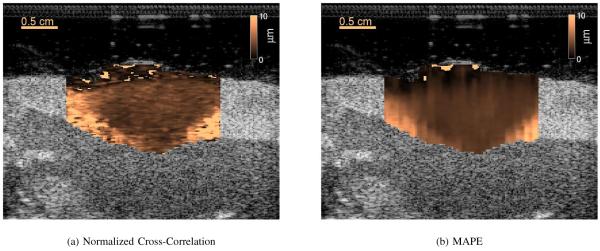
An In vivo comparison of unbiased and biased ARFI images of a cryoablation lesion (copper scale) embedded in a BMode image (grayscale). The first image shows an image of the cryoablation lesion with displacements estimated using normalized cross-correlation. The same data is used to create the second image, but the displacements are estimated using the MAPE. The contrasts of the normalized cross-correlation and MAPE derived displacement images are 0.4370 and 0.3988, respectively. The CNRs of the normalized cross-correlation and MAPE derived images are 0.2534 and 0.6236, respectively. The MAPE image on the right shows subtle vertical displacement streaks resulting from the parallel tracking sequence in conjunction with the early time step after the initial push used to form this image. Because the image is created at an early time after excitation there has not been sufficent time for the shear wave to propagate away from the initial excitation position and a banding artifact results. This effect is also present in the image on the left, but the artifact is masked by the larger variance of the unbiased estimator.
The contrasts of the ARFI image made using normalized cross-correlation and MAPE are 0.4370 and 0.3988, respectively. The contrast-to-noise ratios (CNR) for the ARFI image made with normalized cross-correlation and MAPE are 0.2534 and 0.6236, respectively4. (The CNR calculated for the MLE derived ARFI image may seem low based on the visibility of the lesion, but the image has been saturated on the high displacement end. Image saturation significantly improves the effective CNR.)
One downside side of Bayesian speckle tracking—as implemented here—is that the final result is influenced by the starting position of the prior scheme. Worse results have been seen when the prior scheme starts outside of the tissue, which could occur because it starts above the myocardium in the standoff pad, or because it starts below the myocardium inside the chamber. The dependence on start position is not seen to be a major limiting factor since the important issue seems to be starting at any tissue location.
IV. DISCUSSION
The results presented in this paper are significant but not because of the specific method used to estimate prior probabilities5, but because with a simple prior scheme the Cramer-Rao lower bound can be surpassed. It is entirely expected that within the framework laid out here and in the companion paper [1] displacement estimation performance will continue to improve. This improvement will come from increasingly sophisticated methods for computing prior information [20], [21].
As an example, one of the first ways to realize improved performance is suggested by the results seen from low-pass filtering the unbiased displacements of ARF induced motion6. The ARF induced motion estimates that were low-pass filtered by a long filter had slightly better MSE performance than any of the biased estimates. The low-pass filter appears to be advantaged (at least in part) because it was implemented non-causally (i.e. symmetrically) and unlike the biased estimators was not tethered by a false causality. Forcing a false causality is a common theme in advanced displacement estimation methods [22]–[24] where only estimates before the current estimate are allowed to assist in refining the current estimate. By moving away from this unnecessary constraint, estimator performance will likely improve.
In addition to developing a framework for Bayesian speckle tracking two new estimators were introduced, the minimum mean square estimator and the maximum a posteriori estimator. The usefulness of each estimator is situational. For large search regions—such as in static elastography imaging—MAPE works well particularly if the prior has a large variance. For smaller search regions required for estimating ARFI induced motion the MMSE may work slightly better, particularly for environments with high thermal noise. The MMSE can also be shown to be computationally more efficient if sub-sample estimators are not used in conjunction with the MAPE or MLE.
Finally, biased displacement estimation has only been applied to 1D displacement scenarios. Two and three dimensional realizations of biased displacement estimation can easily be accomplished by extending the normalized cross-correlation function in (6) to two or three dimensions. (The associated value would also change based on the kernel size.) This has been applied succesfully to in vivo cardiac speckle tracking [25].
V. CONCLUSION
Biased estimators were devised using several simple prior schemes, the non-informative prior and a dynamic prior PDF. These prior schemes were coupled with two methods of extracting displacement estimates from posterior distributions, the MMSE and the MAPE. Using the new biased estimators it was shown that with relatively small amounts of additional information the Cramer-Rao lower bound can be surpassed. While the biased estimators obviously contained bias for appropriate selection of the prior PDF the dominate noise mechanism was still the variance of the error.
Fig. 2.

A flowchart for the deterministic implementation of biased estimation described in the methods.
ACKNOWLEDGMENT
The authors would like to thank Ned Danieley for his computer assistance, Marko Jakovljevic for helpful suggestions and Douglas Dumont and Pat Wolf with their assistance in acquiring the in vivo data.
Additionally, the authors would like to thank NIH grants R37HL096023 and T32EB001040 for financial support.
The authors would like to thank NIH grants R37HL096023 and T32EB001040 for funding this research.
APPENDIX. STOCHASTIC VS. DETERMINISTIC IMPLEMENTATIONS
Bayesian estimators are appropriately implemented stochastically. For example, the estimators developed here should be implemented by drawing random values from the prior PDF that describes the a priori knowledge of τ0. However, deterministic approximations can in some cases be faster or at least can be more readily implemented in existing code. It will be shown that appropriate stochastic implementations of the Bayesian estimators and deterministic implementations yield statistically indistinguishable results. The estimators will be implemented deterministically by directly multiplying the prior distribution over τ0 and the likelihood function. In order to make the sampling simple the prior PDF for both cases will always be a normal distribution with mean and variance equivalent to the previous posterior distribution.
Two example results for specific data realizations are shown in Fig. 14. The results show how the random sampled implementation converges to a final estimate as more samples are drawn. The example shows that the deterministic and stochastic implementation for a given realization of data do not necessarily converge to the same result. Results for simulating 1000 data realizations and comparing the displacement estimate error distribution between the two methods is shown in Fig. 15. The figure shows the resulting p-value from statistical tests to compare the mean and variance of the error distributions for the two methods as a function of depth and of number of drawn samples for the stochastic implementation. The results show that only at very shallow depths (i.e. broad prior distribution) and a small number of draws from the prior distribution do the error distributions vary. The exception to this is at deeper depths (i.e. narrow priors) where a small portion of the estimates derived from the stochastic implementation yield large errors, which result in statistically different distributions.
Fig. 14.

This figure shows two example results comparing a deterministic implementation (direct multiplication of PDFs) of the proposed estimator and a true Bayesian implementation (randomly drawing from the prior distribution) for the simple case implemented here. The first example is for a relatively shallow depth with a wide prior probability on τ0. The second example is for still shallow but deeper depth (5 mm), which has a more refined prior.
Fig. 15.

This figure demonstrates the similarity between the deterministic and probabilistic implementations of the biased estimators. The two figures show the actual p-value calculated as a function of the number of samples from the prior and depth.
While the deterministic and stochastic approach are shown to be statistically equivalent for the simple case implemented in this paper, this similarity should not automatically be expected to hold for more complex problems.
Footnotes
The MMSE with either prior scheme shows the same artifact.
Even when MSE improvements over normalized cross-correlation are not realized the prior can still act as a peak-hopping filter. Peak-hopping can be reduced by the prior (as compared to the non-informative prior) by slightly attenuating correlation peaks away from the prior’s mean.
At later times the blockiness goes away as the displacement propagates away from its original lateral location in the form of some transverse wave (e.g. lamb wave, shear wave, etc.).
| (14) |
| (15) |
In the chance that someone imitates the method used here for computing dynamic priors an inherent weakness in the approach is that there is not a good mechanism for allowing the prior PDFs to become wider if the information at an adjacent location appears to be uncorrelated. This is easily observed in the results of the step displacement simulations where small values for σmin result in nearly unrecoverable performance degradation after the step displacement. This will be a function of both the step size and the standard deviation of the prior distribution.
These results where primarily shown in the figure of frequency response, Fig 6. It was observed that a 47th order low-pass filter could produce a better MSE.
REFERENCES
- [1].Byram BC, Trahey GE, Palmeri M. Bayesian speckle tracking. part I: An implementable pertubation to the likelihood function for ultrasound displacement estimation. IEEE Trans. Ultrason. Ferroelect. Freq. Contr. vol. ??(no. 4) doi: 10.1109/TUFFC.2013.2545. ??–??, ?? ?? [DOI] [PMC free article] [PubMed] [Google Scholar]
- [2].Kay SM. Fundamentals of statistical signal processing: estimation theory. Prentice-Hall, Inc.; Upper Saddle River, NJ, USA: 1993. [Google Scholar]
- [3].Embree PM. Ph.D. dissertation. University of Illinois; Urbana, Ill: 1985. The accurate ultrasonic measurement of volume flow of blood by time-domain correlation. [Google Scholar]
- [4].Cespedes I, Insana M, Ophir J. Theoretical Bounds on Strain Estimation in Elastography. IEEE Trans. Ultrason. Ferroelect. Freq. Contr. 1995 Sep;vol. 42(no. 5):969–972. [Google Scholar]
- [5].Walker W, Trahey G. A fundamental limit on the performance of correlation-based phase correction and flow estimation techniques. IEEE Trans. Ultrason. Ferroelect. Freq. Contr. 1994;vol. 41:644–654. [Google Scholar]
- [6]. — A fundamental limit on delay estimation using partially correlated speckle signals. IEEE Trans. Ultrason. Ferroelect. Freq. Contr. 1995;vol. 42(2):301–308. [Google Scholar]
- [7].Lubinski MA, Emelianov SY, Raghavan KR, Yagle AE, Skovoroda AR, O’Donnell M. Lateral displacement estimation using tissue incompressibility. IEEE Trans. Ultrason. Ferroelect. Freq. Contr. 1996;vol. 43:247–256. doi: 10.1109/58.660158. [DOI] [PubMed] [Google Scholar]
- [8].Jaynes ET. Probability Theory: The Logic of Science. Vol 1. Cambridge University Press; Apr, 2003. [Google Scholar]
- [9].Zahiri-Azar R, Salcudean S. Motion estimation in ultrasound images using time domain cross correlation with prior estimates. IEEE Trans. Biomedical Engineering. 2006 Oct.vol. 53(no. 10):1990–2000. doi: 10.1109/TBME.2006.881780. [DOI] [PubMed] [Google Scholar]
- [10].Jiang J, Hall TJ. A parallelizable real-time motion tracking algorithm with applications to ultrasonic strain imaging. Phys. Med. Biol. 2007 Jul;vol. 52(no. 13):3773–3790. doi: 10.1088/0031-9155/52/13/008. [DOI] [PubMed] [Google Scholar]
- [11].Chen L, Housden RJ, Treece GM, Gee AH, Prager RW. A hybrid displacement estimation method for ultrasonic elasticity imaging. IEEE Trans. Ultrason. Ferroelectr. Freq. Control. 2010 Apr;vol. 57(no. 4):866–882. doi: 10.1109/TUFFC.2010.1491. [DOI] [PMC free article] [PubMed] [Google Scholar]
- [12].Schlaikjer M, Jensen JA. Maximum likelihood blood velocity estimator incorporating properties of flow physics. IEEE Trans. Ultrason. Ferroelect. Freq. Contr. 2004;vol. 51(no. 1):80–92. doi: 10.1109/tuffc.2004.1268470. [DOI] [PubMed] [Google Scholar]
- [13].Wagner R, Insana MF, S. W. S. Fundamental correlation lengths of coherent speckle in medical ultrasonic images. IEEE Trans. Ultrason. Ferroelect. Freq. Contr. 1988 Jan;vol. 35(no. 1):34–44. doi: 10.1109/58.4145. [DOI] [PMC free article] [PubMed] [Google Scholar]
- [14].S. P. D. Committe, Programs for Digital Signal Processing. IEEE Press; Piscataway, NJ, USA: 1979. [Google Scholar]
- [15].Varghese T, Ophir J. A theoretical framework for performance characterization of elastography: the strain filter. IEEE Trans Ultrason Ferroelectr Freq Control. 1997;vol. 44(no. 1):164–172. doi: 10.1109/58.585212. [DOI] [PubMed] [Google Scholar]
- [16].Palmeri ML, Sharma AC, Bouchard RR, Nightingale RW, Nightingale KR. A finite-element method model of soft tissueresponse to impulsive acoustic radiation force. IEEE Trans. Ultrason. Ferroelectr. Freq. Control. 2005 Oct;vol. 52(no. 10):1699–1712. doi: 10.1109/tuffc.2005.1561624. [DOI] [PMC free article] [PubMed] [Google Scholar]
- [17].Palmeri ML, McAleavey SA, Trahey GE, Nightingale KR. Ultrasonic tracking of acoustic radiation force-induced displacements in homogeneous media. IEEE Trans. Ultrason. Ferroelectr. Freq. Control. 2006 Jul;vol. 53(no. 7):1300–1313. doi: 10.1109/tuffc.2006.1665078. [DOI] [PMC free article] [PubMed] [Google Scholar]
- [18].Jensen JA, Svendsen NB. Calculation of pressure fields from arbitrarily shaped, apodized and excited ultrasound transducers. IEEE Trans. Ultrason. Ferroelect. Freq. Contr. 1992;vol. 39:262–267. doi: 10.1109/58.139123. [DOI] [PubMed] [Google Scholar]
- [19].Jensen JA. Field: A program for simulating ultrasound systems. Paper presented at the 10th Nordic-Baltic Conference on Biomedical Imaging Published in Medical & Biological Engineering & Computing.1996. pp. 351–353. [Google Scholar]
- [20].Debski W. Advances in Geophysics, ser. Advances in Geophysics. 525 B Street, Suite 1900, San Diego, CA 92101-4495. vol. 52. Elsevier Academic Press, Inc; USA: 2010. Probabilistic Inverse Theory; pp. 1–102. [Google Scholar]
- [21].Rabiner LR. A tutorial on hidden markov models and selected applications in speech recognition. Proceedings of the IEEE. 1989:257–286. [Google Scholar]
- [22].Pellot-Barakat C, Frouin F, Insana M, Herment A. Ultrasound elastography based on multiscale estimations of regularized displacement fields. IEEE Trans. Med. Imaging. 2004 Feb;vol. 23(no. 2):153–163. doi: 10.1109/TMI.2003.822825. [DOI] [PMC free article] [PubMed] [Google Scholar]
- [23].Jiang J, Hall TJ. A generalized speckle tracking algorithm for ultrasonic strain imaging using dynamic programming. Ultrasound Med Biol. 2009;vol. 35(no. 11):1863–79. doi: 10.1016/j.ultrasmedbio.2009.05.016. [DOI] [PMC free article] [PubMed] [Google Scholar]
- [24].Petrank Y, Huang L, O’Donnell M. Reduced peak-hopping artifacts in ultrasonic strain estimation using the viterbi algorithm. IEEE Trans Ultrason Ferroelectr Freq Control. 2009;vol. 56(no. 7):1359–67. doi: 10.1109/TUFFC.2009.1192. [DOI] [PubMed] [Google Scholar]
- [25].Byram BC. Ph.D. dissertation. Duke University; 2011. Chronic myocardial infarct visualization using 3d ultrasound. [Google Scholar]