

Abstract
Optimization methods are presented to design Halbach arrays to maximize the forces applied on magnetic nanoparticles at deep tissue locations. In magnetic drug targeting, where magnets are used to focus therapeutic nanoparticles to disease locations, the sharp fall off of magnetic fields and forces with distances from magnets has limited the depth of targeting. Creating stronger forces at depth by optimally designed Halbach arrays would allow treatment of a wider class of patients, e.g. patients with deeper tumors. The presented optimization methods are based on semi-definite quadratic programming, yield provably globally optimal Halbach designs in 2 and 3-dimensions, for maximal pull or push magnetic forces (stronger pull forces can collect nano-particles against blood forces in deeper vessels; push forces can be used to inject particles into precise locations, e.g. into the inner ear). These Halbach designs, here tested in simulations of Maxwell’s equations, significantly outperform benchmark magnets of the same size and strength. For example, a 3-dimensional 36 element 2000 cm3 volume optimal Halbach design yields a ×5 greater force at a 10 cm depth compared to a uniformly magnetized magnet of the same size and strength. The designed arrays should be feasible to construct, as they have a similar strength (≤ 1 Tesla), size (≤ 2000 cm3), and number of elements (≤ 36) as previously demonstrated arrays, and retain good performance for reasonable manufacturing errors (element magnetization direction errors ≤ 5°), thus yielding practical designs to improve magnetic drug targeting treatment depths.
Keywords: magnetic nano-particles, targeted drug delivery, magnetic drug targeting, optimal permanent magnets, nano-particle trapping, pushing nano-particles, Halbach array design
2. Introduction
Magnetic drug targeting refers to the use of magnets to direct therapeutic magnetizable nano-particles to regions of disease: to tumors [1–3], infections [4] or blood clots [5]. Targeting allows the focusing of drugs [6–15] and other therapies, such as gene therapy [16], to disease locations. Such magnetic targeting can reduce the distribution of drugs to the rest of the body, thus minimizing side effects such as those caused by systemically administered chemotherapy [17–19]. The reach of magnetic drug targeting – the distance from the magnets to in vivo locations where particle capture is still effective – depends, in addition to the vascularization of the targeted region [20–24], on both the applied magnetic field and the magnetic gradient, both of which fall off quickly with distance from magnets [25], [26]. Insufficient reach has limited the applicability of magnetic drug delivery. In cancer, it has limited treatment to shallow tumors [9], [27]. If focusing depth could be increased that would allow treatment of a greater number of disease profiles and patients. The research presented here aims to maximize the reach of magnetic drug delivery [23], [24], [28–30] by designing optimal Halbach arrays [31] to extend magnetic forces deeper into the body.
Existing magnetic drug delivery techniques commonly use permanent magnets or electromagnets to pull particles into the target tissue by placing the magnets in close proximity to the target to accumulate the therapy [32–36]. Magnet strengths have ranged from 70 milliTesla [32] to 2.2 Tesla [36] with corresponding applied magnetic gradients from 3 T/m [33] to 100 T/m [35], a range that reflects desired/possible depth of targeting versus magnet cost, complexity, and ease-of-use. To date, a focusing depth of 5 cm has been achieved in human clinical trials with 100 nm diameter particles using 0.2– 0.8 T strength magnets [8], [9]; and focusing depths of up to 12 cm have been reported in animal experiments using larger 500 nm to 5 μm particles and a 0.5 T permanent magnet [27]. Restricted treatment depths means that only a fraction of patients can be treated with magnetic drug delivery, for example those who present with shallow but inoperable tumors (like the patient shown in Figure 1a). An ability to extend magnetic forces deeper into the body would enable treatment of more patients.
Figure 1.
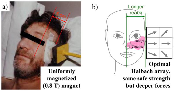
a) Magnetic drug delivery has been limited to 5 cm depths in human trials [1], [9] (photograph taken from [37]). b) Halbach arrays could create deeper magnetic forces using the same magnetic field strengths by optimally shaping the magnetic field (gray arrows show sample magnetization direction in each element of the array).
Figure 1 has a single magnet attracting particles to it. The first optimization goal is to lengthen the reach of such a pull attraction. However, it is also possible to use magnets to push or magnetically inject particles [38]. The ability to magnetically push in particles is valuable for a variety of clinical applications, from non-invasively injecting therapy into the inner ear [39], to pushing drugs to the back of the retina for treatment of eye diseases [32], to injecting nano-therapies into wounds and ulcers [40]. The mathematical methods developed here can be used to optimize both pull and push Halbach designs, and examples for both cases are presented.
Thus the focus of the work described in this article is the optimal design of permanent magnet Halbach arrays for maximally pulling in, and pushing away, magnetizable particles for longer-reach magnetic drug delivery. In contrast to gradient descent [41] or machine-learning-type optimization methods [42], which can get caught in local optima [41], [43], the solutions presented here are globally optimal. In standard fashion [44], global optimality is proved by first finding rigorous upper and lower bounds for the optimized metric (which here is the magnetic force). These upper and lower bounds bracket the true optimal value. For all the cases tested, the upper and lower bounds converged thus squeezing the range of optimal solutions to a single value between them (the global optimum).
The optimization proceeds as follows. The Halbach design problem can be stated from physical first principles as a non-convex constrained quadratic optimization, and this problem can be converted into an equivalent linear constrained optimization by a change of variables. Relaxing one constraint yields a new problem, now convex, whose solution is an upper bound for the original non-convex constrained quadratic problem. This type of constraint relaxation technique is known as semidefinite relaxation (SDR) [45] and it provides a rigorous upper bound – the relaxed-constraints optimum is guaranteed to provide a greater force than (i.e. an upper bound on) the globally-optimal Halbach array because it does not have to meet all the constraints (one of which has been relaxed away, see Section 5). A lower bound is extracted from the upper bound matrix solution of the SDR problem by shrinking the solution matrix eigenvector with the maximum eigenvalue so that a new solution matrix does satisfy all the linear constraints. This yields a solution that satisfies the change-of-variable constraints but that is sub-optimal and therefore provides a rigorous lower bound. The lower bound is then increased by optimizing a modified convex function that approximates the original non-convex quadratic problem. As the optimization proceeds, specific Halbach magnet configurations are found each creating a specific but sub-optimal magnetic force (see open circles in Figure 2). The final design (closed black circle) is squeezed between the lower and upper bounds and is guaranteed to be the globally optimal solution – the best possible Halbach design.
Figure 2.
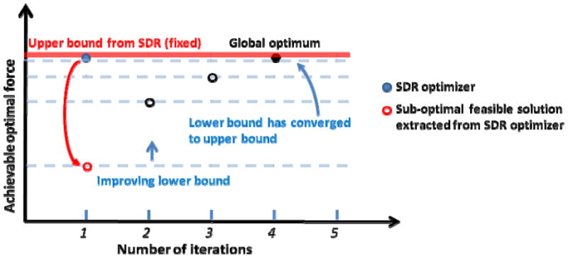
Global optimality is proved by showing that the upper and lower bounds converge, squeezing the optimum design between them. The figure shows upper and lower bounds, as well as the sub-optimal and final optimal force value, for the Halbach optimization case of Section 6.1. At each iteration of the optimization, it is known that the true optimum magnetic force must be less than the upper bound (red line, computed by SDR) and greater than the lower bound (blue line, computed by an approximate convex optimization scheme). As the optimization proceeds, better and better solutions are found, and the bounds are driven closer together eventually converging (here at iteration 4). The shown global optimum (black dot) corresponds to a 36 element Halbach array that creates a magnetic force at a distance of 10 cm that is 71 % greater than the force created by a uniformly magnetized block of the same size and magnetic field strength.
Most magnetic drug targeting systems [33], [34], [46], [47], have relied on pull forces generated by a single permanent magnet placed near the target tissue. Recently, magnet shaping has been employed in the design of permanent magnets [48], [49] and electromagnets [35], [36], [50] to improve magnetic gradients and thus enhance pull forces. Halbach arrays for near surface magnetic focusing have been demonstrated in [28], [51]. To attain longer reach, one of the more notable Halbach magnet optimizations is the Stereotaxis’ Niobe® system to maximally project magnetic forces [52], [53] – a design that has allowed for the steering of catheters and guide wires during magnetically-assisted heart surgery. Implanting of magnetic materials inside patients – within, for example, blood vessel walls – has been proposed in [7], [54], [55] as an alternate way to target drugs to deep tissues. The implanted materials serve to locally increase the magnetic field gradients when an external magnetic field is applied. Finally, superconducting materials have also drawn interest from the research community for generation of stronger magnetic forces [25], [56–59]. However, there are as yet no methods to optimize permanent magnet Halbach arrays to maximize the strength and depth of magnetic pull and push forces. We consider that problem here and design optimal arrays with a reasonable number of elements (36 for all the cases below). Construction of strong Halbach arrays with this many elements is feasible, as has been demonstrated for 1 Tesla arrays with 36 elements in [60].
Since prior human trials have been restricted to a focusing depth of 5 cm [1], [9], and since generating sufficient force at depth remains a challenge [7], [54], [55], [61], we choose as a specific goal throughout this paper to increase magnetic forces at depth. To make the problem concrete, we choose to optimize force at 10 cm for Halbach designs with total volume of 2000 cm3, 36 elements, and each element having a remanence of ≤ 1 Tesla – a size, strength, and number of elements that is feasible to construct. Maximizing pull force at one specific depth also increases forces at surrounding locations (it is not the case that maximizing force at 10 cm leads to a decreased force at 7 cm), and the optimization methods presented here can be trivially extended to optimize the force over a region instead of at a point. For push forces, there is usually a location we want to push at (e.g. through the round window membrane that leads into the inner ear [38]) and so it makes sense to optimize push at that specific location. The optimization leads to designs that substantially outperform uniformly magnetized magnets of the same size, shape, and magnetic field strength.
Specifically, a 2-dimensional flat rectangular 20 cm × 20 cm × 5 cm (2000 cm3 volume) Halbach optimal design with 36 elements created a ×1.45 greater force at a 10 cm distance compared to a benchmark uniformly magnetized magnet of the same size, shape, and strength (Figure 6). The method worked equally well for optimizing Halbach arrays of non-rectangular shapes and, as an example, was demonstrated for a ‘C’ shaped 2-dimensional array (Figure 7). Such a ‘C’ design could be useful for placing the Halbach system around an obstruction, for example around a large tumor that both protrudes out of and extends deeper into the body.
Figure 6.

Optimal 36 element 2D pull array. The black dot identifies the optimization point and the black arrow shows the direction of the pull force at that point. The color indicates the logarithm of the magnetic field strength at that location (for example, a light to medium orange contour of 10.2 corresponds to ||H|| = 1010.2 A/m). The dimensionless factor ‘c’ is the ratio of the pull force for this 36 element optimal Halbach array to the pull force from the benchmark uniform magnet of Figure 5. Each element has a height, width, and thickness of h = 3.33 cm, w = 3.33 cm, and t = 5 cm. The magnetizations of the array “fan in” as this formation focuses the magnetic field and its gradient to the optimization point to create a maximum force.
Figure 7.

Optimal magnetization directions for a ‘C’-shaped 36 element Halbach array. The coloring scheme here is the same as in Figure 6. The magnetizations of the block on the left fan in to concentrate the magnetic field and its gradient at the optimization point, whereas the blocks on the top and bottom provide a flux return and add to the horizontal component of the force.
For magnetic push designs, a 36 element optimized Halbach array was compared against a 2-element push magnet benchmark (since no single element alone can push) and created a force that is ×9 greater at a distance of 10 cm (Figure 11). This is directly relevant for optimizing magnetic injection forces to deliver therapy into the inner ear [38], which is at a distance of 6–10 cm from the surface of the human face. The same optimization methods also worked for optimizing 3-dimensional Halbach designs, for both pull and push scenarios (as shown in Section 7, Figure 12 and Figure 13).
Figure 11.

Optimal shape and magnetization for a 36 element push Halbach array with the same volume as the benchmark array of Figure 9. Here the shape optimization has selected elements closest to the optimization point but in two separate halves. The 8 most-central elements orient to induce a cancellation node, while the rest fan-in to focus the magnetic field and its gradient beyond the cancellation node in order to generate the strongest push force. The factor ‘d’ is the ratio of the push force for this optimal array versus the benchmark 2-element array. The coloring scheme is the same as used in Figure 6.
Figure 12.
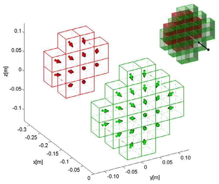
Plot showing the optimal geometry and magnetization directions for a 36 element 3D Halbach pull array (with the same volume as the benchmark pull magnet shown in Figure 5). Each element is a cube with every side measuring 3.816 cm. The two layers of the Halbach array along the x-axis (front layer shown in green, rear in red) are shown apart to better visualize the magnetization directions. The overall formation of the array is shown at top right where the two layers are right next to each other and the optimization point and resulting force are shown by the black dot and arrow. The 2-layer “pyramid” shape is again optimal because the most effective elements are the ones closest to the optimization point. Also as before, the magnetization directions “fan in”, like in Figure 8, to push out and focus the magnetic field to better include the optimization point.
Figure 13.
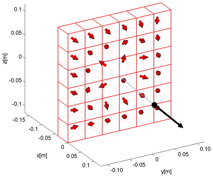
Plot showing the geometry and magnetization directions for a 36 element 3D Halbach array push design (having the same overall volume as that of the benchmark Halbach array of Figure 9). Each sub-magnet is a cube with every side measuring 3.816 cm. The optimization point and resulting force are shown by the black dot and arrow. The elements closest to the optimization point orient to induce a cancellation node like in Figure 11, while the rest focus to extend the magnetic field and its gradient beyond the cancellation node in order to generate a strong push force.
We were also able to extend our techniques to optimize the shape of Halbach arrays. Instead of choosing a prescribed shape, like a ‘C’ shape of Figure 7 or the rectangle shape of Figure 1a, and then finding optimal magnetization directions for each element within that shape; we were able to find the optimal placement of the elements. This was done by including one additional constraint in the optimization that effectively selected the N best placed elements from a larger grid of M elements thus revealing the optimal shape (see the end of Section 5), and this was done in both 2 and 3-dimensions, for both pull and push. Three-dimensional, 36 element, 2000 cm3 volume Halbach designs, with both optimal element placement and magnetization directions, are demonstrated in Figure 12 and Figure 13, and they create push and pull forces at a 10 cm distance that are ×5 and ×26 greater than the benchmark magnets of the same volume and strength.
Finally, to check that our optimal Halbach designs are practical, we considered a 5° degree error in magnetization directions, as would be reasonable during array fabrication. We found that the push and pull forces are sufficiently insensitive to these manufacturing errors for the designs to remain practical (see Section 8).
3. Physics for Magnetic Fields and Forces
To design the Halbach arrays, we need to quantify the magnetic fields and forces they create. Magnetic fields are described by Maxwell’s equations [62]. Since the designs discussed here utilize stationary permanent magnets, the magneto-static equations are appropriate. These are
| (1) |
| (2) |
| (3) |
where B⃑ is the magnetic field [in Tesla], H⃗ is the magnetic intensity [A/m], j⃗ is the current density [A/m2] and is zero in our case, M⃗ is the material magnetization [A/m], χ is the magnetic susceptibility, and μo = 4 π × 10−7 N/A2 is the permeability of vacuum. These equations hold true in vacuum as well as in materials (air or liquid), and for electromagnets and permanent magnets (magnetization M⃗ ≠ 0). The resulting force on a single ferro-magnetic particle is then
| (4) |
where a is the radius of the particle [m], ∇ is the gradient operator [with units 1/m], and ∂H⃑/∂x⃗ is the Jacobian matrix of H⃑ both evaluated at the location of the particle [7], [63–65]. The first relation states that the force on a single particle is proportional to its volume and the gradient of the magnetic field intensity squared – i.e. a ferro-magnetic particle will always experience a force from low to high applied magnetic field. The second relation, which is obtained by applying the chain rule to the first one, is more common in the magnetic drug delivery literature and shows that a spatially varying magnetic field (∂H⃑/∂x⃑ ≠ 0) is required to create a magnetic force. Thus, in order to maximize the force experienced by a given particle, the gradient of the magnetic field squared must be maximized. This is the only term controlled by the magnet design; all other terms depend on the size and material properties of the particles.
4. Problem Formulation
Consider a Halbach array composed of permanent rectangular sub-magnets arranged in a rectangular formation, each magnetized uniformly in a given direction. The optimization task is to select the magnetization directions to maximize pull or push forces on particles located at a specific distance from the magnet. Figure 3 shows a schematic of a 2-dimensional Halbach array sample. As illustrated, the goal is to choose the optimal magnetization directions (indicated by the blue arrows) to maximize the pull or push magnetic force at (x0,y0). Deep reach can be optimized by maximizing the pull or push forces at a (x0,y0) location far from the Halbach array.
Figure 3.
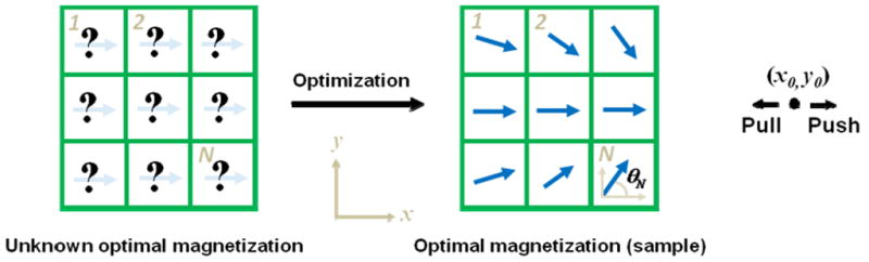
Schematic of Halbach array of N magnets arranged in rectangle formation. Each green box represents a sub-magnet. The blue arrows show possible magnetization directions. The goal is to find the angle θ for each sub-magnet in order to maximize the push or pull force at the location (x0,y0).
If the strength of the Halbach array is unrestricted, then the magnetic force can be increased simply by making the magnets stronger. However, there are practical constraints on the available strengths of permanent magnets as well as regulatory safety constraints on the strength of the magnetic field that can be applied across the human body (the United States Food and Drug Administration currently considers 8 T fields safe for adults and up to 4 T appropriate for children [66]). Thus the desired optimization problem is to maximize the magnetic force given a maximum allowable magnetic field strength. For convenience, and since permanent NdFeB magnets can be purchased with remanence magnetization of around one Tesla, we limit the magnetization of each Halbach element to 1 Tesla.
The magnetic field around a uniformly magnetized rectangular magnet is known analytically. Here the analytical expression developed by Herbert and Hesjedal [67] is used to express the magnetic field around a Halbach array with sub-magnets having arbitrary magnetization directions. The magnetic field from two or more magnets can be added together to establish the net magnetic field. This is a standard assumption in the design of Halbach arrays [31], and it is true as long as the magnetic field arising from the combination of sub-magnets does not cause partial or complete demagnetization or magnetization reversals [68]. The designs we present in this paper do not generate demagnetizing fields strong enough to cause partial or complete demagnetization of the sub-magnets involved.
Let A⃗(x, y) represent the analytical expression for the magnetic field around a rectangular magnet that is uniformly magnetized along the positive horizontal axis, and let B⃗(x, y) represent the analytical expression for the same magnet uniformly magnetized along the positive vertical axis. Then the magnetic field when this magnet is uniformly magnetized at an angle θ is given by A⃗(x, y)cosθ +B⃗(x, y)sinθ. The magnetic field around the entire Halbach array is generated by translating and adding together solutions for all the elements. For the ith Halbach element at location (ai,bi), with (as yet unspecified) magnetization direction θi, let αi = cosθi and βi = sinθi. The magnetic field created at location (x0,y0) by this element is
| (5) |
The coefficients αi and βi are the unknown design variables. In order to limit the strength of any given element to one Tesla, the constraint is imposed for all i. For a Halbach array containing N sub-magnets, the expression for the magnetic field at point (x0,y0) is
| (6) |
The relationship between the design variables αi and βi and the magnetic force exerted by the Halbach array at point (x0,y0) is quadratic in the variables αi and βi. According to equation (4), the strength of the magnetic force experienced by a magnetic particle at a point (x0,y0) is directly proportional to the gradient of the square of the magnetic field at that point. Define
| (7) |
and
| (8) |
Squaring equation (6) and taking the gradient, the expression for ∇H⃗2 (x0, y0) becomes
| (9) |
The gradient operator ∇ is linear. Since the coefficients αi and βi are not functions of x and y they can be pulled out of the summation. The resulting equation (10) shows how the magnetic force of equation (4) depends on the Halbach array design variables αi and βi:
| (10) |
The Halbach array optimization problem can now be stated in matrix form. The goal is to maximize magnetic pull or push forces along the horizontal axis and, thus, the focus is solely on the horizontal component of ∇H⃗2 (x0, y0), i.e. (∇H⃗2 (x0, y0))x:=∇H⃗2 (x0, y0)·(1,0). Define the matrix P as
| (11) |
and define the vector q⃗ as a concatenated list of the design variables αi and βi as
| (12) |
Now (∇H⃗2 (x0, y0))x can be written in compact form as
| (13) |
This equation succinctly states how the horizontal magnetic force strength depends on the Halbach design variables. To include the magnetization constraints, let Gi be a 2N ×2N matrix having unity at the locations (i,i) and (N +i, N +i), and with zeros everywhere else. Then the element magnetization constraints can be written in matrix form as
| (14) |
for all i. The force optimization problem can, therefore, be stated as follows: maximize (for push) or minimize (for pull) the quadratic cost q⃗T Pq⃗ of equation (13) subject to the N constraints of equation (14), one for each Halbach element (for i = 1, 2, … N).
5. Problem Solution
The quadratic optimization problem formulated in the last section (also referred to as a quadratic program) can be solved using various methods. It is not convex – the matrix P is not necessarily negative or positive semi-definite – which implies that it can have many local optima and hence a globally optimal solution cannot be guaranteed in general. Much of the literature on non-convex quadratic programming has focused on obtaining good local minima, using nonlinear programming techniques [69] such as active-set or interior-point methods [70]. Numerous general-purpose optimization techniques can also be tailored to solve quadratic programs. A review of several optimization methods for non-convex quadratic programs can be found in [71] and [72]. Some machine learning methods – such as those based on neural networks [42] – have also been used to solve this class of problems. However, for non-convex problems, these methods often get stuck in local optima [41], [43].
We employ a combination of 2 methods to find the optimal solutions and determine the upper and lower bounds for the optimal force: 1) semi-definite relaxation [73] and 2) the majorization method [74]. Rigorous bounds provide information on the quality of the optimal solution. If, for example, it is known that the maximum achievable force is guaranteed to be between FL and FU, and the found optimum has a force F in the top range of the bracket close to FU, then the found solution is a high quality optimum close to the true (global) maximum. If, as in Figure 2, and as occurs for all the Halbach optimization cases in this paper, the two bounds converge, then we additionally know for certain that a global optimum has been achieved.
To find the upper bound for a maximum push (or pull) force, semi-definite relaxation (SDR) [73] is employed. This method converts the original non-convex quadratic problem into a closely related convex problem by a change of variables and a constraint relaxation. Finding a solution to the new SDR problem is much easier, is numerically more efficient, and a global optimum to the relaxed, changed-variables problem is guaranteed [73]. The global optimum of the relaxed SDR problem is an upper bound for the global optimum of the original non-convex quadratic problem (this upper bound is illustrated as the red line in Figure 2).
To compute the lower bound, rescaling the above SDR solution to satisfy the constraints yields a solution, a magnet design, that satisfies all the constraints but that is sub-optimal (the first open circle at iteration 1 in Figure 2) – this solution is a lower bound for the global optimum of the original non-convex quadratic program (bottom most dashed gray line). The scaled sub-optimal solution can then be improved by optimizing a convex function that approximates the original non-convex cost function. The solution to this approximate constrained convex problem leads to an improved sub-optimal solution (second open circle in Figure 2) and provides a tighter lower bound (higher dashed gray line). The next iteration yields a third sub-optimal solution and a better third lower bound. The process repeats until no further improvement is possible or until the lower bound reaches the upper bound proving that a global optimum of the original problem has been found.
Below we first discuss the mathematical details of the relaxed-constraint convex SDR process and the upper bound that it yields. Then we describe the iteration of approximate convex problems that gives a succession of sub-optimal solutions and improved lower bounds. When these lower bounds converge to the upper bound the last solution is guaranteed to be the global optimum Halbach design.
The mathematics is presented for optimizing push. Maximizing pull proceeds in exactly the same way except that the cost function q⃗T Pq⃗ is replaced by its negative −q⃗T Pq⃗ and this oppositely signed function is then minimized. The conversion from the original non-convex problem to a convex matrix problem is achieved by a change of variables. The SDR corresponding to the original optimization problem of equations (13) and (14) can be re-stated as follows. The P and Gi matrices are symmetric. For symmetric matrices
| (15) |
| (16) |
where the trace operator Tr(·) is the sum of the elements on the main diagonal of a square matrix. Define the new matrix variable Q:= q⃗q⃗T as the outer product of the q⃗ vector with itself. This recasts the cost and constraints into linear functions of Q
| (17) |
| (18) |
however, not all Q’s are permissible. Only Q matrices that can be formed by the outer product of a single vector, i.e. of the form Q:= q⃗q⃗T should be considered, and this is the set of matrices that are positive semidefinite (Q ≥ 0) with unit rank [75]. Thus the optimization can be rephrased as maximize or minimize Tr(PQ) subject to the N+2 constraints: Tr(GiQ) ≤ 1 for i = 1,2, … N; Q ≥ 0; and rank(Q) = 1. The cost and the first N+1 constraints are convex in Q [45]. However, the last rank constraint is not convex. If this rank constraint is removed then the problem becomes convex and a global optimum can be readily found. Removing the rank constraint allows a wider choice of Q solutions: it includes the Q:= q⃗q⃗T case but also allows other solutions that are not the outer product of a single vector. Thus the cost attained by solving this new convex problem is guaranteed to match or exceed the cost that can be achieved for the original non-convex constrained quadratic problem – if Q* is the global optimal solution to the relaxed convex problem with achieved cost Tr(PQ*), and q⃗* is the (still unknown) global solution to the original quadratic problem of equations (13) and, then it is guaranteed that q⃗ *T Pq⃗* ≤Tr(PQ*). Thus Tr(PQ*) is an upper bound to the true global optimum (it is the red line in Figure 2).
The optimal solution Q* of the relaxed convex problem also provides a lower bound to the true global optimum after an appropriate rescaling. Let v⃗* be the eigenvector of Q* that has the maximum eigenvalue. In order for v⃗* to qualify as a suboptimal feasible solution to the original non-convex quadratic problem, it must satisfy the N constraints v⃗*T Gi v⃗* ≤ 1 for all i = 1, 2, …, N. Let τ be the maximum value that the expression v⃗* Gi v⃗* achieves for all i, so define . By definition v⃗*T Gi v⃗* ≤ τ for all i. Now let then so this new scaled vector q⃗ satisfies the N constraints q⃗#T Gi q⃗# ≤ 1 for all i = 1, 2, … N. It is therefore a feasible suboptimal solution to the original non-convex quadratic program. A sub-optimal solution cannot beat the maximum possible pull or push force and is therefore a guaranteed lower bound to the original problem, i.e. q⃗*T P q⃗* ≥ q⃗#T P q⃗#. This first lower bound is shown by the lowest dashed gray line in Figure 2.
The task now is to improve the lower bound. Any vector q⃗ that satisfies the constraints of the original problem yields at least a sub-optimal solution, and hence provides a lower bound to the optimal magnetic force. In order to further improve the lower bound achieved by q⃗#, the original quadratic problem is approximated with a convex function without relaxing any constraints. This convex function is formulated in such a way that optimizing it also produces an optimal (but possibly local) solution to the original quadratic problem.
To define this new convex function, we proceed as follows. Note that maximizing q⃗T Pq⃗ is equivalent to minimizing f (q⃗):= −q⃗TPq⃗. Define the new function F(q⃗), which is called the convex quadratic majorizer [74] of f (q⃗) at q⃗#, as
| (19) |
where ∇ denotes the gradient operator with respect to q⃗, ∇f (q⃗)|q⃗# is the gradient of f (q⃗) with respect to q⃗ and then evaluated at q⃗#, λ = max[0, λmax (P)], and λmax(P) denotes the maximum eigenvalue of the matrix P. That the function F is a convex quadratic majorizer of f at q⃗# means that f (q⃗) ≤ F(q⃗) for all q⃗, and f (q⃗) = F(q⃗) for q⃗ =q⃗# [74]. If q⃗## minimizes F, then we have the sandwich inequality f (q⃗##) ≤ F (q⃗##) ≤F (q⃗#) = f (q⃗#). The first inequality shows that minimizing F implies decreasing the value of the objective function f (q⃗), which is equivalent to increasing the value of q⃗T Pq⃗.
Unlike f, the function F is convex in q⃗ because f (q⃗#) is a constant offset, (q⃗ −q⃗#)T ∇f (q⃗)|q⃗# is linear in q⃑, and λ(q⃗−q⃗#)T (q⃗−q⃗#) is purely quadratic with λ ≥ 0. Thus the new approximate problem: minimize F (q⃗) subject to the same constraints as the original problem q⃗T Giq⃗ ≤1 for i = 1, 2, … N, is convex and its global optimum q⃗## can be found. Since F is only an approximation to the true cost f = −q⃗T Pq⃗, its global optimum is a feasible but sub-optimal solution of the original non-convex problem. As such, it provides the next lower bound q⃗*T Pq⃗* ≥ q⃗##T Pq⃗##. This second lower bound is shown as the second dashed blue line in Figure 2. At the next iteration, q⃗# is replaced by q⃗## in F of equation (19), a new sub-optimal solution q⃗### is found, and the process repeats until the lower bound cannot be improved any further. In Figure 2 this occurs at the 4th iteration, and the final Halbach array design vector q⃗* = q⃗#### has a lower bound that achieves the upper bound proving that q⃗* = q⃗#### is a global optimum of the original non-convex constrained optimization problem – it is the best possible solution of the Halbach design problem posed in Figure 3 and equations (13) and (14).
In addition to optimizing magnetization directions for a fixed Halbach array shape (as in Figure 3 for a rectangular array), it also possible to use the same methods to choose optimal array shapes. The additional key idea is simple and is shown in Figure 4. Suppose we want to design an optimal Halbach array, in shape and magnetization directions, using only N magnets. A grid of M magnets is considered where M > N and an optimization is used to determine the sub-set of N magnets that are most significant – this determines the shape of the array (step 1 in the figure). The second step is to then re-compute the optimal magnetization directions for this shape. Together, this finds a magnet design that has both the best shape and the best magnetization directions for a specified magnet volume (equivalently for a restricted number of magnet elements).
Figure 4.
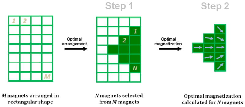
Design of Halbach array with optimal shape and magnetization. Step 1: consider M sub-magnets arranged in a rectangular shape larger than the desired magnet, then find the N most significant sub-magnets that maximize the force (push or pull) at (x0,y0). Step 2: Given these N sub-magnets, find their respective magnetization so that force (push or pull) is maximized at (x0,y0).
Mathematical formulation of Step 1, to select the best N out of M elements, is very similar to what has already been done. The new part is to effectively restrict the number of elements to just N, and this can be done by adding a single new constraint. As before, we maximize (for push) or minimize (for pull) the quadratic cost q⃗T Pq⃗, as shown in equation (13), but now for M (>N) sub-magnets. Hence we state M constraints q⃗T Giq⃗ ≤1 (for i=1,2,…,M) as we still want to limit the strength of each element to 1 Tesla. One additional constraint effectively restricts the number of magnets back to only N by requiring the sum of the squares of all the design variables αi and βi to be less than N, i.e., . Dividing by N, this new constraint can be written in matrix form (remember that the vector q⃗ now has length 2M) as
| (20) |
where G is the identity matrix of size 2M. When this optimization is solved as before, we select the N sub-magnets with the greatest values of to conclude step 1. Then step 2 proceeds exactly as before except now the rectangular arrangement of elements in Figure 3 is replaced by the new arrangement of array elements determined in step 1. The end result is both an optimal array shape and element magnetization directions.
6. Optimized 2D Halbach Array Designs
In this section we begin to show the results of the optimization methods. We start with arrays of a fixed shape (no shape optimization yet) and present various designs of optimized 2-dimensional Halbach arrays for maximum pull and push force objectives. In line with the problem formulated in Section 4, it is assumed that the array elements can only be magnetized in the xy plane. Magnetization along the z-axis is set to zero. In all of the designs presented, the force is optimized at a distance of 10 cm from the edge of the array. This allows for meaningful comparisons to be made. Various designs to achieve maximum pull forces are discussed first.
6.1. Maximum Pull Force Designs
Maximizing the pull force translates to minimizing the horizontal force, making it as negative as possible. Since the goal is to see if the optimized Halbach arrays can perform better than a simple uniformly magnetized magnet, for example as used in [47], all designs are benchmarked against such a rectangular magnet of the same size and 1 Tesla magnet strength. Considering a benchmark magnet of 20 cm height, 20 cm width, and 5 cm thickness, the reference point (the desired point for optimizing the force in a Halbach array of the same dimensions) is chosen at a horizontal distance of 10 cm from the vertical right edge of the magnet (as shown in Figure 5).
Figure 5.
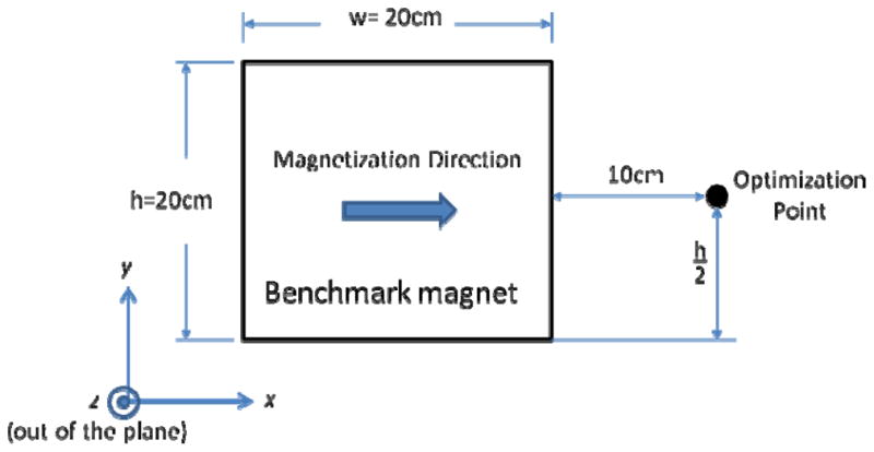
Benchmark magnet. Schematic showing the axis system and chosen optimization location for a benchmark uniformly magnetized rectangular magnet with height h = 20 cm, width w =20 cm, and thickness t = 5 cm. The optimization point is located at x = 10 cm, y = h/2 cm, and z = t/2 cm. This magnet is used as a benchmark for both the 2D and 3D pull design cases.
Recall that the magnetic force (pull or push) is proportional to the horizontal component of the gradient of the magnetic field squared: (∇H⃗2 (x0, y0))x. The benchmark rectangular magnet has (∇H⃗2 (x0, y0))x = −4.39× 10¹⁰ A2/m3, with the negative sign indicating a pull force.
Figure 6 illustrates the optimal magnetization directions for a planar 36 element Halbach array with the same overall shape (rectangle) and volume as the benchmark magnet of Figure 5. The force was optimized at a point 10 cm away from the right most face of the array. The pull force generated by this optimal 2-dimensional Halbach design is ×1.45 more than that generated by the benchmark uniform magnet of the same strength and volume. The optimization to determine this design took 4 minutes to run on a computer with an Intel® Core™ i7 processor with 8GB of RAM using MATLAB version 7.9.0.
Next we show that the optimization method works equally well for other pre-determined shapes besides a rectangle. As an example, we consider a ‘C’ shape with the same volume as the benchmark magnet shown in Figure 5 and again optimize with 36-elements (again of identical size) the pulling force at a distance of 10 cm. Such a ‘C’ shape could be appropriate for placing a Halbach array around a protrusion from the body such as a large tumor that extends out of as well as into the body. The optimal ‘C’ array shown in Figure 7 generates a pull force that is ×2.16 more than that generated by the uniformly magnetized benchmark magnet, and it enables a 49% improvement in force over the optimal rectangular array of Figure 6 demonstrating that array geometry can play a significant role in improving magnetic forces. This case also took 4 minutes to run on the same computer (Intel® Core™ i7 processor, 8GB of RAM using MATLAB version 7.9.0).
Figure 8 illustrates both the optimal shape and magnetization directions for a planar 36 element Halbach array with the same volume as the benchmark magnet of Figure 5. To find the optimal placement of the 36 elements, a grid of M = 18 × 18 = 324 elements was considered, and the 36 most significant elements were chosen by the optimal element selection method described earlier. The force was optimized at a point 10 cm away from the right most face of the array. The pull force generated by this optimal 2-dimensional Halbach design shown in Figure 8 is ×1.71 more than that generated by the benchmark uniform magnet of the same strength and volume. This case took 17 minutes to optimize.
Figure 8.

Plot showing the optimal arrangement and magnetization directions (indicated using large maroon arrows) for a 36 element Halbach array with the same volume as the benchmark magnet. The coloring scheme here is the same as in Figure 6. Intuitively, the shape optimization has elected to keep those elements that are closest to the black optimization point creating a “pyramid” shape. As seen before, the magnetization directions fan in to concentrate the magnetic field and its gradient at the optimization point. This 2D optimal shape and magnetization array increases the pull force by 71% compared to the benchmark magnet.
6.2. Maximum Push Force Designs
Although a single magnetic element will always attract nanoparticles towards itself, a correct arrangement of just two elements can push – and thus magnetically inject – particles. Magnetic pushing is useful for a variety of clinical applications such as magnetically injecting therapy into wounds, infections, or inner ear diseases [38]. Pushing works by creating a magnetic cancellation node at a distance. Magnetic forces then radiate outwards from that cancellation causing a push force on the far side of the node (see [38] for details). As for pull applications, there is a need to optimize magnet arrangements to reach deeper, push harder, and to do so with shaped arrays that can be fit around obstructions or minimized in size so they can be inserted into confined spaces.
Maximizing push is equivalent to maximizing the cost function of equation (13). (For pull we minimized this function.) It is not possible to benchmark pushing against a single uniformly magnetized magnet, since such a single element will always pull particles towards itself. Instead the push designs are benchmarked against a minimal Halbach array consisting of just two rectangular magnets, one on top of the other (see Figure 9), with a remanence of 1 Tesla each. The overall dimensions of the array are the same as that of the benchmark pull magnet shown in Figure 5 (w = 20 cm, h = 20 cm, and t = 5 cm). For this 2-element push benchmark we have (∇H⃗2 (x0, y0))x = + 2.94×10⁸A2/m3 at a distance of 10 cm with the positive sign indicating the push force.
Figure 9.

The push benchmark magnet. Since a single element cannot push, we use a minimal 2-element design as the benchmark with the magnetization directions optimally chosen to create a push at a 10 cm distance. The coloring scheme here is the same as in Figure 6.
Figure 10 illustrates the optimal magnetization directions for a planar 36 element Halbach array with the same overall shape (rectangle) and volume as the benchmark push array of Figure 9. The force was optimized at a location 10 cm away from the right most face of the array. The push force generated by this optimal 2-dimensional Halbach design shown in Figure 10 is ×4.81 more than that generated by the benchmark push array of same magnetic field strength and volume. This case took 4 minutes to run on the computer as before.
Figure 10.

Optimal magnetization for a 36 element Halbach push array with the same volume as the benchmark array of Figure 9. Each element has dimensions of h = 3.33cm, w = 3.33 cm, and t = 5 cm. The factor ‘d’ is the ratio of the push force for this optimal array versus the benchmark 2-element array. The coloring scheme is the same as used in Figure 6. The elements closer to the optimization point orient to induce a cancellation node, while the rest align to extend magnetic field and its gradient beyond the cancellation node to generate a maximal push force.
Next we show optimization of both element placing and magnetization directions for maximal pushing at a 10 cm distance. We consider a 36 element array of the same strength and volume as the push benchmark magnet of Figure 9. To find the optimal shape, the optimization selected N = 36 most significant elements from a grid of M = 18 × 18 = 324 elements. The optimal array is shown in Figure 11 and generates a push force that is more than nine times that of the benchmark array of the same strength and volume. This case took 17 minutes to evaluate.
7. Optimized 3D Halbach Arrays
The previous optimization results were stated in 2 spatial dimensions only. We now consider optimizing 3 dimensional arrays. The mathematics remains the same: the problem statement of Section 4 readily generalizes to the 3rd dimension, and is still solved as described in Section 5. Geometry can now be optimized in three dimensions, and each sub-magnet element can be magnetized by a vector that has components in all three directions. As before, in all of the 3-dimensional designs the force is optimized at a distance of 10 cm from the face of the array to allow for meaningful comparison with the associated 2-dimensional cases.
7.1. Maximum Pull Force Design
A pull force optimization is carried out for a 36 element (each element a cube) 3 dimensional Halbach array having the same overall volume as that of the benchmark magnet of Figure 5. To find the optimal shape, the optimization selected the N = 36 most significant elements from a grid of M = 3 × 10 × 10= 300 elements. As the elements farther away from the optimization location are less significant, only 3 layers were picked along the horizontal axis for the grid. The optimal array shape is shown in Figure 12. The force generated by this design at the optimization point is about 5 times greater than that generated by the benchmark magnet shown in Figure 5. The added degrees of freedom along the z-axis, therefore, provide significant improvement in the design of Halbach arrays for pull force applications. This case took 1 hour and 43 minutes to run on the same computer as previously (Intel® Core™ i7 processor, 8GB of RAM, using MATLAB version 7.9.0).
7.2. Maximum Push Force Design
Comparable to the 3 dimensional pull force design described above, a push force optimization is also carried out for a 36 element (each element a cube) 3 dimensional Halbach array of the same strength and volume as the push benchmark magnet of Figure 9. To find the optimal shape, the optimization selected the N = 36 most significant elements from a grid of M = 3 × 10 × 10 = 300 elements. The optimal array is shown in Figure 13. The force generated by this design at the optimization point is about 26 times greater than that generated by the benchmark magnet shown in Figure 9. As seen for the pull force design, the added degrees of freedom along the z-axis also provide significant improvement in the design of Halbach arrays for push force applications. This case took 1 hour and 43 minutes to optimize.
8. Sensitivity Analysis of Push and Pull Designs
A sensitivity analysis was carried out to determine how errors in element magnetization angles will affect the array pull and push forces. This analysis is included to quantify the effect of inevitable manufacturing imperfections on the performance of the arrays. It was found that the pull force designs were robust to perturbations in magnetization angles. For each pull case, ten independent runs were carried out to capture the extent of variations in the forces. Randomly generated perturbations of up to 5° were introduced in the magnetization angles of each design, simulating reasonable tolerances and variations in the manufacturing of Halbach arrays. The resultant pull forces only showed a variation of 0.3% in magnitude, with a maximum pull force angle deviation of 0.5° away from the horizontal. This indicates that the pull designs are quite robust to reasonable magnetization manufacturing errors.
Push force design is more sensitive to magnetization angle errors. In a series similar to the one above, ten independent runs were carried out for each push force design in order to quantify the variations in push forces. Randomly generated perturbations of up to 5° were introduced in the magnetization angles of each design. The resultant push forces strayed away from the horizontal by up to 4° on the average, and 8° in the most extreme cases. However, the magnitude of forces along the horizontal axis exhibited a maximum decrease of only 0.8%. In contrast, the magnitude of forces along the vertical axis (these were originally zero) rose significantly – to 13.2% of the nominal magnitude of the horizontal component of the push forces. This was expected since push relies on a magnetic field cancellation and that cancellation was anticipated to be more sensitive to magnetization direction errors, and it implies that more care must be taken in the manufacturing and arrangement of magnets for push force applications than for pull cases.
9. Conclusion
Methods based on semi-definite quadratic programming have been presented to optimize Halbach arrays to maximize push and pull forces on magnetic particles at depth. These methods provide rigorous upper and lower bounds on optimality and for all the array shapes tested, these bounds converged proving that the found magnetization directions were globally optimal solutions. The optimizations ran in minutes for 2-dimensional arrays, and in less than 2 hours for 3D arrays, on a desktop PC using MATLAB. They were appropriate to maximize either pull or push forces at depth for any prescribed array shapes. An additional constraint and selection of N out of M most significant elements further allowed the determination of the optimal shapes of Halbach arrays, in addition to their optimal magnetization directions. The presented case study designs should be feasible to construct (they are in line with previously constructed 36 element 1 Tesla arrays), and were sufficiently insensitive to magnetization direction errors even for the more sensitive push cases to remain practical under anticipated manufacturing errors. These designs substantially outperformed benchmark magnets of the same size and magnetic field strength with magnetic push and 3D designs showing the most benefits. Since depth of treatment is one of the key limitations for magnetic drug targeting, the presented capabilities should provide a path towards the construction of safe and practical Halbach arrays to reach deeper tissue targets and thus enable magnetic treatment of a wider set of patients.
Optimization methods presented to design Halbach arrays for drug targeting
The goal is to maximize forces on magnetic nanoparticles at deep tissue locations.
The presented methods yield provably globally optimal Halbach designs in 2D and 3D
These designs significantly outperform benchmark magnets of the same size and strength.
These designs retain good performance for reasonable manufacturing errors (≤ 5°)
Footnotes
Publisher's Disclaimer: This is a PDF file of an unedited manuscript that has been accepted for publication. As a service to our customers we are providing this early version of the manuscript. The manuscript will undergo copyediting, typesetting, and review of the resulting proof before it is published in its final citable form. Please note that during the production process errors may be discovered which could affect the content, and all legal disclaimers that apply to the journal pertain.
References
- 1.Lübbe AS, Alexiou C, Bergemann C. Clinical Applications of Magnetic Drug Targeting. Journal of Surgical Research. 2001 Feb;95(2):200–206. doi: 10.1006/jsre.2000.6030. [DOI] [PubMed] [Google Scholar]
- 2.Pulfer SK, Ciccotto SL, Gallo JM. Distribution of small magnetic particles in brain tumor-bearing rats. Journal of Neuro-Oncology. 1999 Jan;41(2):99–105. doi: 10.1023/a:1006137523591. [DOI] [PubMed] [Google Scholar]
- 3.Jurgons R, Seliger C, Hilpert A, Trahms L, Odenbach S, Alexiou C. Drug loaded magnetic nanoparticles for cancer therapy. Journal of Physics: Condensed Matter. 2006 Sep;18(38):S2893–S2902. [Google Scholar]
- 4.Taylor EN, Webster TJ. Multifunctional magnetic nanoparticles for orthopedic and biofilm infections. International Journal of Nanotechnology. 2011;8(1/2):21–35. [Google Scholar]
- 5.Kempe M, et al. The use of magnetite nanoparticles for implant-assisted magnetic drug targeting in thrombolytic therapy. Biomaterials. 2010 Dec;31(36):9499–9510. doi: 10.1016/j.biomaterials.2010.07.107. [DOI] [PubMed] [Google Scholar]
- 6.Bawa R. Nanoparticle-Based Therapeutics in Humans: A Survey. Nanotechnology Law & Business. 2008;5:135. [Google Scholar]
- 7.Forbes ZG, Yellen BB, Barbee KA, Friedman G. An approach to targeted drug delivery based on uniform magnetic fields. IEEE Transactions on Magnetics. 2003 Sep;39(5):3372–3377. [Google Scholar]
- 8.Lübbe AS, et al. Preclinical Experiences with Magnetic Drug Targeting: Tolerance and Efficacy. Cancer Research. 1996 Oct;56(20):4694–4701. [PubMed] [Google Scholar]
- 9.Lübbe AS, et al. Clinical Experiences with Magnetic Drug Targeting: A Phase I Study with 4′-Epidoxorubicin in 14 Patients with Advanced Solid Tumors. Cancer Research. 1996 Oct;56(20):4686–4693. [PubMed] [Google Scholar]
- 10.Ruuge E, Rusetski A. Magnetic fluids as drug carriers: Targeted transport of drugs by a magnetic field. Journal of Magnetism and Magnetic Materials. 1993 Apr;122(1–3):335–339. [Google Scholar]
- 11.Lübbe A. Physiological aspects in magnetic drug-targeting. Journal of Magnetism and Magnetic Materials. 1999 Apr;194(1–3):149–155. [Google Scholar]
- 12.Alexiou C, et al. Magnetic drug targeting--biodistribution of the magnetic carrier and the chemotherapeutic agent mitoxantrone after locoregional cancer treatment. Journal of Drug Targeting. 2003 Apr;11(3):139–149. doi: 10.1080/1061186031000150791. [DOI] [PubMed] [Google Scholar]
- 13.Lemke A-J, Senfft von Pilsach M-I, Lubbe A, Bergemann C, Riess H, Felix R. MRI after magnetic drug targeting in patients with advanced solid malignant tumors. European Radiology. 2004 Aug;14(11):1949–1955. doi: 10.1007/s00330-004-2445-7. [DOI] [PubMed] [Google Scholar]
- 14.Alexiou C, Jurgons R, Seliger C, Kolb S, Heubeck B, Iro H. Distribution of Mitoxantrone after Magnetic Drug Targeting: Fluorescence Microscopic Investigations on VX2 Squamous Cell Carcinoma Cells. Zeitschrift für Physikalische Chemie. 2006 Feb;220(2_2006):235–240. [Google Scholar]
- 15.Xiong P, Guo P, Xiang D, He JS. Theoretical research of magnetic drug targeting guided by an outside magnetic field. 2006;55:4383–4387. [Google Scholar]
- 16.Dobson J. Gene therapy progress and prospects: magnetic nanoparticle-based gene delivery. Gene Ther. 0000;13(4):283–287. doi: 10.1038/sj.gt.3302720. [DOI] [PubMed] [Google Scholar]
- 17.Allen JC. Complications of chemotherapy in patients with brain and spinal cord tumors. Pediatric Neurosurgery. 1992. 1991;17(4):218–224. doi: 10.1159/000120601. [DOI] [PubMed] [Google Scholar]
- 18.Schuell B, et al. Side effects during chemotherapy predict tumour response in advanced colorectal cancer. British Journal of Cancer. 2005 Oct;93(7):744–748. doi: 10.1038/sj.bjc.6602783. [DOI] [PMC free article] [PubMed] [Google Scholar]
- 19.Devita VT. Cancer: Principles and Practice of Oncology Single Volume. 5. Lippincott Williams & Wilkins; 1997. [Google Scholar]
- 20.Chertok B, et al. Iron oxide nanoparticles as a drug delivery vehicle for MRI monitored magnetic targeting of brain tumors. Biomaterials. 2008 Feb;29(4):487–496. doi: 10.1016/j.biomaterials.2007.08.050. [DOI] [PMC free article] [PubMed] [Google Scholar]
- 21.Sun C, Lee JSH, Zhang M. Magnetic nanoparticles in MR imaging and drug delivery. Advanced Drug Delivery Reviews. 2008 Aug;60(11):1252–1265. doi: 10.1016/j.addr.2008.03.018. [DOI] [PMC free article] [PubMed] [Google Scholar]
- 22.Dobson J. Magnetic nanoparticles for drug delivery. Drug Development Research. 2006;67(1):55–60. [Google Scholar]
- 23.Nacev A, Beni C, Bruno O, Shapiro B. The behaviors of ferromagnetic nano-particles in and around blood vessels under applied magnetic fields. Journal of Magnetism and Magnetic Materials. 2011 Mar;323(6):651–668. doi: 10.1016/j.jmmm.2010.09.008. [DOI] [PMC free article] [PubMed] [Google Scholar]
- 24.Nacev A, Beni C, Bruno O, Shapiro B. Magnetic nanoparticle transport within flowing blood and into surrounding tissue. Nanomedicine (London, England) 2010 Nov;5(9):1459–1466. doi: 10.2217/nnm.10.104. [DOI] [PMC free article] [PubMed] [Google Scholar]
- 25.Takeda S-ichi, Mishima F, Fujimoto S, Izumi Y, Nishijima S. Development of magnetically targeted drug delivery system using superconducting magnet. Journal of Magnetism and Magnetic Materials. 2007 Apr;311(1):367–371. [Google Scholar]
- 26.Rotariu O, Strachan NJC. Modelling magnetic carrier particle targeting in the tumor microvasculature for cancer treatment. Journal of Magnetism and Magnetic Materials. 2005 May;293(1):639–646. [Google Scholar]
- 27.Goodwin S, Peterson C, Hoh C, Bittner C. Targeting and retention of magnetic targeted carriers (MTCs) enhancing intra-arterial chemotherapy. Journal of Magnetism and Magnetic Materials. 1999 Apr;194:132–139. [Google Scholar]
- 28.Häfeli UO, Gilmour K, Zhou A, Lee S, Hayden ME. Modeling of magnetic bandages for drug targeting: Button vs. Halbach arrays. Journal of Magnetism and Magnetic Materials. 2007 Apr;311(1):323–329. [Google Scholar]
- 29.Voltairas PA, Fotiadis DI, Michalis LK. Hydrodynamics of magnetic drug targeting. Journal of Biomechanics. 2002 Jun;35(6):813–821. doi: 10.1016/s0021-9290(02)00034-9. [DOI] [PubMed] [Google Scholar]
- 30.Grief AD, Richardson G. Mathematical modelling of magnetically targeted drug delivery. Journal of Magnetism and Magnetic Materials. 2005 May;293(1):455–463. [Google Scholar]
- 31.Halbach K. Design of permanent multipole magnets with oriented rare earth cobalt material. Nuclear Instruments and Methods. 1980 Feb;169(1):1–10. [Google Scholar]
- 32.Holligan DL, Gillies GT, Dailey JP. Magnetic guidance of ferrofluidic nanoparticles in an in vitro model of intraocular retinal repair. Nanotechnology. 2003 Jun;14(6):661–666. [Google Scholar]
- 33.Ally J, Martin B, Behrad Khamesee M, Roa W, Amirfazli A. Magnetic targeting of aerosol particles for cancer therapy. Journal of Magnetism and Magnetic Materials. 2005 May;293(1):442–449. [Google Scholar]
- 34.Alexiou C, Jurgons R, Seliger C, Brunke O, Iro H, Odenbach S. Delivery of superparamagnetic nanoparticles for local chemotherapy after intraarterial infusion and magnetic drug targeting. Anticancer Research. 2007 Aug;27(4):2019–2022. [PubMed] [Google Scholar]
- 35.Dames P, et al. Targeted delivery of magnetic aerosol droplets to the lung. Nat Nano. 2007;2(8):495–499. doi: 10.1038/nnano.2007.217. [DOI] [PubMed] [Google Scholar]
- 36.Alexiou C, et al. A High Field Gradient Magnet for Magnetic Drug Targeting. IEEE Transactions on Applied Superconductivity. 2006 Jun;16(2):1527–1530. [Google Scholar]
- 37.Lubbe AS. Personal Communication (photograph from one of the patients from the clinical trials of A S Lubbe et al, [1996]) May, 2007.
- 38.Shapiro B, Dormer K, Rutel IB. A Two-Magnet System to Push Therapeutic Nanoparticles. AIP Conference Proceedings. 2010 Dec;1311(1):77–88. doi: 10.1063/1.3530064. [DOI] [PMC free article] [PubMed] [Google Scholar]
- 39.Kopke RD, et al. Magnetic Nanoparticles: Inner Ear Targeted Molecule Delivery and Middle Ear Implant. Audiology and Neurotology. 2006;11(2):123–133. doi: 10.1159/000090685. [DOI] [PubMed] [Google Scholar]
- 40.Cortivo R, Vindigni V, Iacobellis L, Abatangelo G, Pinton P, Zavan B. Nanoscale particle therapies for wounds and ulcers. Nanomedicine (London, England) 2010 Jun;5(4):641–656. doi: 10.2217/nnm.10.32. [DOI] [PubMed] [Google Scholar]
- 41.Bertsekas DP, Bertsekas DP. Nonlinear Programming. 2. Athena Scientific; 1999. [Google Scholar]
- 42.Cichocki A, Unbehauen R. Neural Networks for Optimization and Signal Processing. 1. Wiley; 1993. [Google Scholar]
- 43.Zhang X-S. Neural networks in optimization. Springer; 2000. [Google Scholar]
- 44.Floudas CA, Pardalos PM. Encyclopedia of Optimization. 1. Springer; 2001. [Google Scholar]
- 45.Boyd S, Vandenberghe L. Convex Optimization. Cambridge University Press; 2004. [Google Scholar]
- 46.Ally J, Amirfazli A, Roa W. Factors affecting magnetic retention of particles in the upper airways: an in vitro and ex vivo study. Journal of Aerosol Medicine: The Official Journal of the International Society for Aerosols in Medicine. 2006;19(4):491–509. doi: 10.1089/jam.2006.19.491. [DOI] [PubMed] [Google Scholar]
- 47.Zebli B, Susha AS, Sukhorukov GB, Rogach AL, Parak WJ. Magnetic Targeting and Cellular Uptake of Polymer Microcapsules Simultaneously Functionalized with Magnetic and Luminescent Nanocrystals. Langmuir. 2005 May;21(10):4262–4265. doi: 10.1021/la0502286. [DOI] [PubMed] [Google Scholar]
- 48.Yang Y, Jiang JS, Du B, Gan ZF, Qian M, Zhang P. Preparation and properties of a novel drug delivery system with both magnetic and biomolecular targeting. Journal of Materials Science Materials in Medicine. 2009 Jan;20(1):301–307. doi: 10.1007/s10856-008-3577-0. [DOI] [PubMed] [Google Scholar]
- 49.Lohakan M, Junchaichanakun P, Boonsang S, Pintavirooj C. A Computational Model of Magnetic Drug Targeting in Blood Vessel using Finite Element Method. 2nd IEEE Conference on Industrial Electronics and Applications, 2007. ICIEA; 2007; 2007. pp. 231–234. [Google Scholar]
- 50.Slabu I, Röth A, Schmitz-Rode T, Baumann M. Optimization of magnetic drug targeting by mathematical modeling and simulation of magnetic fields. In: Sloten J, Verdonck P, Nyssen M, Haueisen J, editors. 4th European Conference of the International Federation for Medical and Biological Engineering. Vol. 22. Berlin, Heidelberg: Springer Berlin Heidelberg; 2009. pp. 2309–2312. [Google Scholar]
- 51.Hayden ME, Häfeli UO. ‘Magnetic bandages’ for targeted delivery of therapeutic agents. Journal of Physics: Condensed Matter. 2006 Sep;18(38):S2877–S2891. [Google Scholar]
- 52.Creighton FM, Ritter RC, Werp P. Focused magnetic navigation using optimized magnets for medical therapies. Magnetics Conference, 2005. INTERMAG Asia 2005. Digests of the IEEE International; 2005. pp. 1253–1254. [Google Scholar]
- 53.Creighton FM. Optimal Distribution of Magnetic Material for Catheter and Guidewire Cardiology Therapies. Magnetics Conference, 2006. INTERMAG 2006. IEEE International; 2006. pp. 111–111. [Google Scholar]
- 54.Polyak B, et al. High field gradient targeting of magnetic nanoparticle-loaded endothelial cells to the surfaces of steel stents. Proceedings of the National Academy of Sciences. 2008 Jan;105(2):698–703. doi: 10.1073/pnas.0708338105. [DOI] [PMC free article] [PubMed] [Google Scholar]
- 55.Yellen BB, Forbes ZG, Barbee KA, Friedman G. Model of an approach to targeted drug delivery based on uniform magnetic fields. Magnetics Conference, 2003. INTERMAG 2003. IEEE International; 2003. p. EC- 06. [Google Scholar]
- 56.Mishima F, Takeda S, Izumi Y, Nishijima S. Development of Magnetic Field Control for Magnetically Targeted Drug Delivery System Using a Superconducting Magnet. IEEE Transactions on Applied Superconductivity. 2007 Jun;17(2):2303–2306. [Google Scholar]
- 57.Fukui S, et al. Study on optimization design of superconducting magnet for magnetic force assisted drug delivery system. Physica C: Superconductivity. 2007 Oct;463–465:1315–1318. [Google Scholar]
- 58.Nishijima S, et al. Research and Development of Magnetic Drug Delivery System Using Bulk High Temperature Superconducting Magnet. IEEE Transactions on Applied Superconductivity. 2009 Jun;19(3):2257–2260. [Google Scholar]
- 59.Haverkort JW, Kenjereš Optimizing drug delivery using non-uniform magnetic fields: a numerical study. IFMBE Proceedings; 2009. pp. 2623–2627. [Google Scholar]
- 60.Zhang X, et al. Design, construction and NMR testing of a 1 tesla Halbach. Permanent Magnet for Magnetic Resonance. presented at the COMSOL Users Conference; Boston, MA. 2005. [Google Scholar]
- 61.Zheng J, Wang J, Tang T, Li G, Cheng H, Zou S. Experimental study on magnetic drug targeting in treating cholangiocarcinoma based on internal magnetic fields. The Chinese-German Journal of Clinical Oncology. 2006 Sep;5(5):336–338. [Google Scholar]
- 62.Feynman RP. The Feynman Lectures on Physics (3 Volume Set) Addison Wesley Longman; 1970. [Google Scholar]
- 63.Fleisch D. A Student’s Guide to Maxwell’s Equations. 1. Cambridge University Press; 2008. [Google Scholar]
- 64.Forbes ZG, Yellen BB, Halverson DS, Fridman G, Barbee KA, Friedman G. Validation of high gradient magnetic field based drug delivery to magnetizable implants under flow. IEEE Transactions on Bio-Medical Engineering. 2008 Feb;55(2 Pt 1):643–649. doi: 10.1109/TBME.2007.899347. [DOI] [PubMed] [Google Scholar]
- 65.Shapiro B. Towards dynamic control of magnetic fields to focus magnetic carriers to targets deep inside the body. Journal of magnetism and magnetic materials. 2009 May;321(10):1594–1594. doi: 10.1016/j.jmmm.2009.02.094. [DOI] [PMC free article] [PubMed] [Google Scholar]
- 66.Chakeres DW, de Vocht F. Static magnetic field effects on human subjects related to magnetic resonance imaging systems. Progress in Biophysics and Molecular Biology. 2005 Apr;87(2–3):255–265. doi: 10.1016/j.pbiomolbio.2004.08.012. [DOI] [PubMed] [Google Scholar]
- 67.Engel-Herbert R, Hesjedal T. Calculation of the magnetic stray field of a uniaxial magnetic domain. Journal of Applied Physics. 2005;97(7):074504. [Google Scholar]
- 68.Katter M. Angular dependence of the demagnetization stability of sintered Nd-Fe-B magnets. Magnetics Conference, 2005. INTERMAG Asia 2005. Digests of the IEEE International; 2005. pp. 945–946. [Google Scholar]
- 69.Burer S, Vandenbussche D. A finite branch-and-bound algorithm for nonconvex quadratic programming via semidefinite relaxations. Mathematical Programming. 2006 Dec;113(2):259–282. [Google Scholar]
- 70.Gould NIM, Toint PL. Numerical Methods for Large-Scale Non-Convex Quadratic Programming. 2001 [Google Scholar]
- 71.Pardalos PM. Global optimization algorithms for linearly constrained indefinite quadratic problems. Computers & Mathematics with Applications. 1991;21(6–7):87–97. [Google Scholar]
- 72.Horst R, Pardalos PM. Handbook of Global Optimization. 1. Springer; 1994. [Google Scholar]
- 73.Luo Zhi-quan, Ma Wing-kin, So AM-C, Ye Yinyu, Zhang Shuzhong. Semidefinite Relaxation of Quadratic Optimization Problems. IEEE Signal Processing Magazine. 2010 May;27(3):20–34. [Google Scholar]
- 74.de Leeuw J, Lange K. Sharp Quadratic Majorization in One Dimension. Computational statistics & data analysis. 2009 May;53(7):2471–2484. doi: 10.1016/j.csda.2009.01.002. [DOI] [PMC free article] [PubMed] [Google Scholar]
- 75.Lay DC. Linear Algebra and Its Applications. 4. Addison Wesley; 2011. [Google Scholar]