

Abstract
Background
To evaluate long-term health outcomes among childhood cancer survivors, St. Jude Children’s Research Hospital (SJCRH) has established the St. Jude Lifetime Cohort (SJLIFE), comprised of adult survivors who undergo risk-directed clinical assessments. As in any human research study, SJLIFE participants are volunteers who may not represent the source population from which they were recruited. A lack of proportional representation could result in biased estimates of exposure-outcome associations. We compared available demographic, disease, and neighborhood level characteristics between participants and the source population to assess the potential for selection bias.
Procedures
Potentially eligible patients for SJLIFE were enumerated as of October 31, 2011. Data from electronic medical records were combined with geocoded census data to develop an analytic data set of 3,108 patients (the evaluable source population) of whom 1766 (57%) underwent clinical assessment (participants). The ratio of relative frequencies (RRF) for characteristics was compared between participants and the source population, where RRF=1.0 indicates equal frequency of the characteristic.
Results
Participants and the source population had similar frequencies for most characteristics. Characteristics with modest relative differences (RRFs between 0.86 and 1.11) included sex, distance from SJCRH, primary diagnosis, median household income, median home value, and urbanicity.
Conclusions
Our results indicate a lack of substantive differences in the relative frequencies of demographic, disease, or neighborhood characteristics between participants and the source population in SJLIFE, thus alleviating serious concerns about selective non-participation in this cohort. Bias in specific exposure-outcome relations is still possible and will be considered in individual analyses.
Keywords: epidemiology, bias, cancer survivorship
INTRODUCTION
Survival rates for most childhood cancers have increased dramatically over the past 40 years[1]. More than 363,000 individuals who were diagnosed with cancer as a child or adolescent were alive in the United States as of January 1, 2009 [2]. Long-term follow-up of survivors is essential for identifying evolving conditions that affect health and functioning throughout the life course [3]. Seminal cohort studies, including the Childhood Cancer Survivor Study (CCSS) [4], have been able to identify treatment- and diagnosis-specific long-term adverse effects of childhood cancer. Nevertheless, the depth of knowledge and interpretation of findings offered from survey-based studies such as CCSS is somewhat limited because of the nature of self-reported data. To facilitate the evaluation of long-term health outcomes among childhood cancer survivors, St. Jude Children’s Research Hospital (SJCRH) recently established a cohort of adult survivors, the St. Jude Lifetime Cohort Study (SJLIFE). This study involves risk-directed clinical assessment for prevalent health-related conditions, medical record review, and survey-based data collection [5]. As of October 31, 2011, SJLIFE had recruited more than 1,700 adult survivors of childhood cancer for comprehensive clinical evaluations.
Participants in any human research study are select volunteers who may or may not accurately represent the distribution of characteristics in the source population (i.e. eligible participants) from which they were identified and recruited. A study population comprised of participants that are systematically different (i.e., the differences are non-random) from the source population raises concerns about potential selection bias [6–9]. The consequence of selection bias is that the estimate of an exposure-outcome association of interest among study participants may be over- or underestimated relative to what would have been found if all eligible individuals participated in the study. Such bias is particularly important to consider in light of the declining participation rates in epidemiologic cohort studies over the past 30 years – from 80% to 30–40% on average [10,11]. Unfortunately, direct assessment of the magnitude of bias from differential participation is rarely possible because information on exposures, outcomes, and relevant covariates are generally unavailable for eligible non-participants. However, when source population data are available, the frequencies of general characteristics can be compared between participants and the source population to broadly assess differential representation in the study [8,12]. The aim of our analysis was to compare the frequency of demographic, disease, and neighborhood characteristics among SJLIFE participants relative to the source population. Additionally, we explored whether a combination of these characteristics could predict participation in an intensive multiple-day clinical research study.
METHODS
St. Jude Lifetime Cohort (SJLIFE)
The study design and cohort characteristics of SJLIFE have been described previously [5]. Briefly, SJLIFE is an IRB-approved institutional cohort study at SJCRH with medical, physical, psychosocial, and neurocognitive assessments conducted to characterize health-related outcomes among adult survivors of childhood cancer [5]. Eligible participants who comprise the source population include living individuals 18 years of age or older who were treated for a pediatric malignancy at SJCRH, and who were diagnosed at least 10 years before enrollment [5]. Individuals who consent to participation in SJLIFE undergo a core battery of evaluations including history and physical examination with resting heart rate, blood pressure, and 12-lead electrocardiography, and laboratory assessments including a complete blood count/differential, comprehensive metabolic panel, urinalysis, and physical performance assessment including formal evaluations of anthropometrics, body composition, aerobic capacity, sensation, flexibility, balance, muscle strength, mobility, and gross and fine motor function. In addition participants received risk-directed clinical and laboratory evaluations according to the Children’s Oncology Group Long Term Follow-up Guidelines [13,14].
Outcome
Our outcome of interest for this analysis was participation in SJLIFE. The SJLIFE study uses a dynamic cohort design [7], which is characterized by a rolling admission process. For example, individuals can become eligible for enrollment in SJLIFE when the eligibility criteria are satisfied even if they were ineligible at study initiation, and eligible participants can consent to enrollment regardless of time since initial eligibility or initial contact. Given the potential for ambiguity about what constitutes a participant in a dynamic cohort, we explicitly defined a participant as an eligible individual who completed the comprehensive on-site medical assessments by October 31, 2011. Non-participants thus included individuals who declined to participate, who completed the survey questionnaires but declined to participate in the on-site medical assessments, who were lost to follow-up, or who were contacted before September 1, 2011 but had not completed a clinical assessment as of October 31, 2011.
Variables
Institutional medical records that contained demographic data, information on childhood cancer diagnosis, and most recent contact information were available for all individuals eligible for SJLIFE (i.e. the source population). Therefore, we were able to designate and ascertain a common set of variables, which included demographic, disease, and neighborhood-level characteristics, for participants and non-participants, which were then de-identified for statistical analysis. We ascertained individual-level demographic characteristics including age of the individual at the original contact mailing date, sex, and race. Individual-level characteristics about childhood cancer diagnosis included primary cancer diagnosis group, age at primary cancer diagnosis, years from primary cancer diagnosis to the contact mailing date, and treatment era.
To enhance the lack of complete individual-level socioeconomic information in the institutional medical records, we used geographic information systems (GIS) mapping software to derive neighborhood-level socioeconomic characteristics based on the most recent contact address for each eligible individual. Briefly, we used ArcGIS software (Environmental Systems Research Institute [ESRI], Redlands, CA) [15] to geolocate residential addresses for eligible individuals. We subsequently linked the geolocation with U.S. census block group-level data from the 2005–2009 American Community Survey (ACS) [16] for each eligible individual with a United States address. Census block groups, subsets of census tracts generally comprised of 600–3000 individuals, provide the most detailed small-area census data publically available [17]. Linkage with the ACS data allowed us to ascertain neighborhood-level educational attainment, household income, home value, and distance in miles from the individual’s reported address to SJCRH. Additionally, we linked geolocations with Rural-Urban Commuting Area (RUCA) data [18] based on zip code information to classify urbanicity [19] for each eligible individual. Post office box addresses, military post office box addresses, and international addresses could not be geocoded and thus were not included in this analysis.
Data analysis
To compare the frequency of demographic, disease, and neighborhood characteristics among SJLIFE participants relative to the source population of SJLIFE, we first computed the relative frequencies (RFs) of these characteristics in the participant and source populations, respectively (i.e. the proportion of the characteristic within each population). We subsequently computed the ratio of relative frequencies (RRFs) for each characteristic, where RRF=RFParticipants/RFSourcePopulation. An RRF=1 indicates that a particular characteristic had equal frequency within the participant and source populations. Nonparametric bootstraps with replacement (n=1,000 random samples of the observed data) were used to estimate 95% confidence limits (CL) for each RRF [20].
To explore whether the combination of demographic, disease, and neighborhood characteristics could predict participation in SJLIFE, we fitted overall and sex-specific unconditional logistic regression models comparing participants and non-participants. These models included individual-level characteristics such as sex (for the overall model), race, age at childhood cancer diagnosis, primary childhood cancer diagnosis group, treatment era, distance in miles from the individual’s reported address to SJCRH, and neighborhood-level characteristics such as educational attainment, median household income, median home value, and urbanicity. We assessed performance of the overall and sex-specific prediction models with estimates of discrimination (i.e. differentiation of participants from non-participants) and calibration (i.e. accuracy of predicted probabilities) [21]. Discrimination was evaluated by estimating the area under the receiver operator curve (AUC), where AUC=1.0 indicates perfect discrimination [21]. Calibration was evaluated by examining the Hosmer-Lemeshow goodness of fit statistic, where P<0.05 suggests poor calibration [21].
Sensitivity analysis
We recognized the potential for the RRFs to be sensitive to the exclusion of eligible individuals with uninformative addresses from the analysis. Although uninformative addresses (including post office boxes and international addresses) precluded determining neighborhood-level characteristics for these individuals, demographic and disease characteristics were available for analysis. Therefore, we used available data to estimate RRFs that compared the relative frequencies of demographic and disease characteristics between participants and the complete source population. The resulting RRFs were compared to the RRFs from the main analysis, which was restricted to eligible individuals for whom neighborhood-level characteristics could be determined, to assess sensitivity to the exclusion of eligible individuals with uninformative addresses.
RESULTS
Figure 1 describes the derivation of participants and non-participants from all individuals potentially eligible for SJLIFE. Briefly, 4,234 childhood cancer survivors were identified through institutional records as potentially eligible as of October 31, 2011, but 686 (16%) were determined to be ineligible or had not yet been contacted for recruited. Thus, 3,548 individuals comprised the source population for this analysis. We were unable to determine geolocations for 440 (12%) individuals in the source population because of international (n=79) or uninformative addresses (e.g., post office boxes; n=361). Therefore, our evaluable source population comprised 3,108 individuals eligible for SJLIFE, of whom 1,766 (57%) were complete participants (i.e. completed the on-site medical assessments and the primary health survey).
Figure 1.
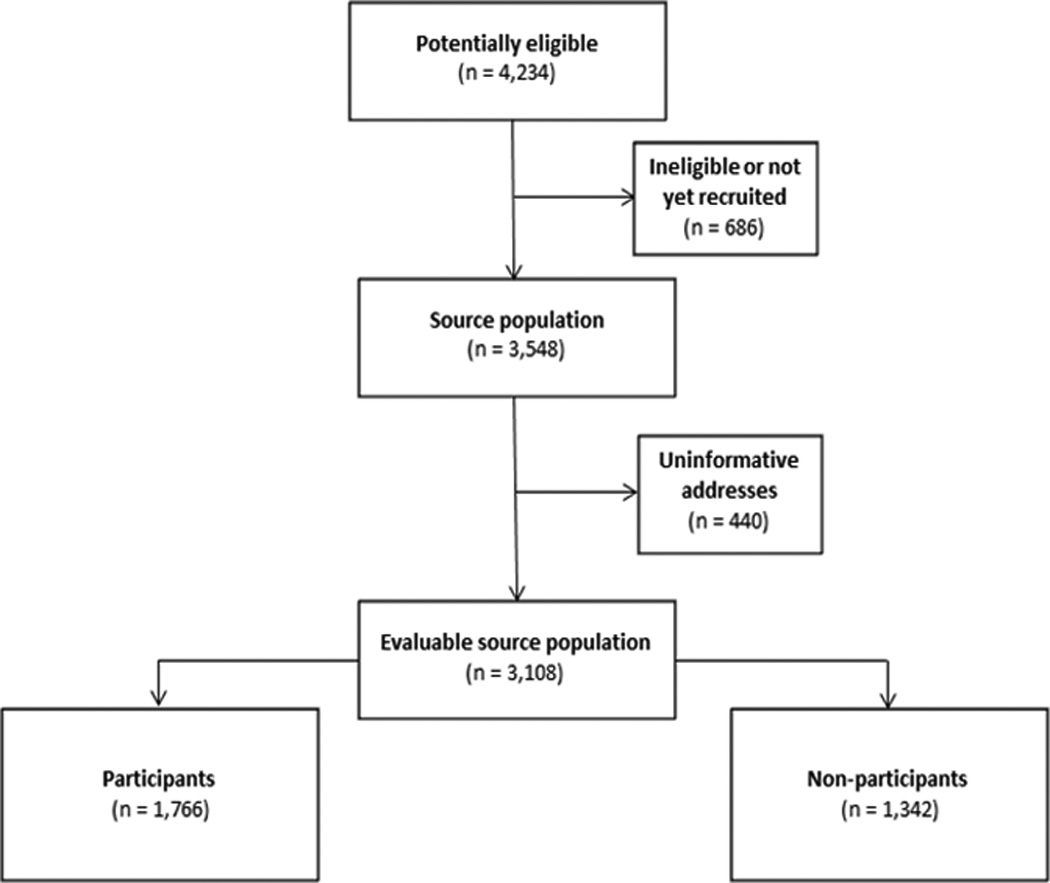
Consort diagram
Table I summarizes overall RRFs comparing the relative frequencies of demographic, disease, and neighborhood characteristics between participants and the evaluable source population. Most characteristics of the participants and the evaluable source population had similar frequencies (i.e. RRF~1). Notable differences in the magnitude of relative frequencies were observed for sex (males: RRF=0.93, 95% CL: 0.90, 0.96; females: RRF=1.08, 95% CL: 1.04, 1.12), distance from SJCRH (0–100 miles: RRF=1.08, 95% CL: 1.02, 1.15), primary diagnosis group (leukemia: RRF=1.11, 95% CL: 1.07, 1.16), treatment era (1970–1979: RRF=1.06, 95% CL: 1.00, 1.12), neighborhood median household income (≥$60,000: RRF=1.08, 95% CL: 1.02, 1.13), neighborhood median home value ($150,000-$199,000: RRF=1.09, 1.01, 1.16), and urbanicity (Rural: RRF=0.86, 95% CL: 0.71, 1.01).
Table 1.
Ratio of relative frequencies (RRFs) for demographic, disease, and neighborhood characteristics between participants in the SJLIFE and the evaluable source population as of October 31, 2011.
| Evaluable source population (N=3,108) |
Participants (n=1,766) |
RRF | 95% confidence limits |
||||
|---|---|---|---|---|---|---|---|
| N | % | n | % | Lower | Upper | ||
| Individual-level characteristics | |||||||
| Sex | |||||||
| Males | 1667 | 53.6 | 882 | 49.9 | 0.93 | 0.90 | 0.96 |
| Females | 1441 | 46.4 | 884 | 50.1 | 1.08 | 1.04 | 1.12 |
| Race | |||||||
| White | 2672 | 86.0 | 1536 | 87.0 | 1.01 | 1.00 | 1.03 |
| Non-White | 436 | 14.0 | 230 | 13.0 | 0.93 | 0.84 | 1.02 |
| Age at contact date | |||||||
| 18 – 30 | 1401 | 45.1 | 789 | 44.7 | 0.99 | 0.95 | 1.03 |
| 31 – 40 | 1160 | 37.3 | 674 | 38.2 | 1.02 | 0.98 | 1.07 |
| ≥ 41 | 547 | 17.6 | 303 | 17.2 | 0.97 | 0.90 | 1.05 |
| Distance from home to SJCRHa (miles) | |||||||
| 0 – 100 | 652 | 21.0 | 401 | 22.7 | 1.08 | 1.02 | 1.15 |
| 101 – 250 | 761 | 24.5 | 412 | 23.3 | 0.95 | 0.89 | 1.02 |
| 251– 500 | 1214 | 39.1 | 671 | 38.0 | 0.97 | 0.93 | 1.01 |
| ≥ 500 | 481 | 15.5 | 282 | 16.0 | 1.03 | 0.95 | 1.11 |
| Age at primary cancer diagnosis | |||||||
| 0 – 2 | 676 | 21.8 | 380 | 21.5 | 0.99 | 0.92 | 1.05 |
| 3 – 5 | 705 | 22.7 | 407 | 23.1 | 1.02 | 0.95 | 1.08 |
| 6 – 8 | 429 | 13.8 | 239 | 13.5 | 0.98 | 0.90 | 1.07 |
| 9 – 11 | 379 | 12.2 | 211 | 12.0 | 0.98 | 0.88 | 1.08 |
| 12 – 14 | 424 | 13.6 | 247 | 14.0 | 1.03 | 0.93 | 1.12 |
| 15 – 17 | 378 | 12.2 | 215 | 12.1 | 1.00 | 0.90 | 1.10 |
| ≥ 18 | 117 | 3.8 | 67 | 3.8 | 1.01 | 0.82 | 1.19 |
| Years from diagnosis to contact date | |||||||
| 10–14 | 283 | 9.1 | 169 | 9.6 | 1.05 | 0.94 | 1.16 |
| 15 – 19 | 585 | 18.8 | 332 | 18.8 | 1.00 | 0.92 | 1.07 |
| 20 – 24 | 745 | 24.0 | 427 | 24.2 | 1.01 | 0.95 | 1.07 |
| 25 – 29 | 672 | 21.6 | 374 | 21.2 | 0.98 | 0.92 | 1.05 |
| 30 – 34 | 445 | 14.3 | 248 | 14.0 | 0.98 | 0.89 | 1.07 |
| 35 – 39 | 262 | 8.4 | 157 | 8.9 | 1.05 | 0.94 | 1.17 |
| ≥ 40 | 116 | 3.7 | 59 | 3.3 | 0.90 | 0.72 | 1.07 |
| Disease group | |||||||
| Bone tumors | 202 | 6.5 | 124 | 7.0 | 1.08 | 0.95 | 1.22 |
| CNS tumors | 247 | 8.0 | 137 | 7.8 | 0.98 | 0.86 | 1.09 |
| Embryonal tumors | 556 | 17.9 | 278 | 15.7 | 0.88 | 0.80 | 0.95 |
| Leukemias | 1219 | 39.2 | 769 | 43.5 | 1.11 | 1.07 | 1.16 |
| Lymphomas | 645 | 20.8 | 349 | 19.8 | 0.95 | 0.88 | 1.02 |
| Soft tissue sarcomas | 176 | 5.7 | 78 | 4.4 | 0.78 | 0.64 | 0.93 |
| Others | 63 | 2.0 | 31 | 1.8 | 0.87 | 0.61 | 1.13 |
| Treatment era | |||||||
| 1962 – 1969 | 125 | 4.0 | 69 | 3.9 | 0.97 | 0.80 | 1.14 |
| 1970 – 1979 | 723 | 23.3 | 435 | 24.6 | 1.06 | 1.00 | 1.12 |
| 1980 – 1989 | 1318 | 42.4 | 737 | 41.7 | 0.98 | 0.94 | 1.03 |
| 1990 – 2002 | 942 | 30.3 | 525 | 29.7 | 0.98 | 0.93 | 1.03 |
| Group-level Characteristics | |||||||
| Education | |||||||
| ≤ High school diploma/general equivalency diploma | 2390 | 77.0 | 1341 | 75.9 | 0.99 | 0.97 | 1.01 |
| > High school diploma/general equivalency diploma | 718 | 23.1 | 425 | 24.1 | 1.04 | 0.98 | 1.11 |
| Median household income | |||||||
| ≤ $29,999 | 533 | 17.2 | 274 | 15.5 | 0.90 | 0.83 | 0.99 |
| $30,000 – $59,999 | 1775 | 57.1 | 1003 | 56.8 | 0.99 | 0.96 | 1.03 |
| ≥ $60,000 | 800 | 25.7 | 489 | 27.7 | 1.08 | 1.02 | 1.13 |
| Median home value | |||||||
| ≤ $99,999 | 1254 | 40.4 | 671 | 38.0 | 0.94 | 0.90 | 0.98 |
| $100,000 – $149,999 | 841 | 27.1 | 477 | 27.0 | 1.00 | 0.94 | 1.05 |
| $150,000 – $199,999 | 525 | 16.9 | 324 | 18.4 | 1.09 | 1.01 | 1.16 |
| ≥ $200,000 | 488 | 15.7 | 294 | 16.7 | 1.06 | 0.98 | 1.15 |
| Urbanicity | |||||||
| Metropolitan area | 2069 | 66.6 | 1212 | 68.6 | 1.03 | 1.01 | 1.06 |
| Micropolitan area | 485 | 15.6 | 259 | 14.7 | 0.94 | 0.86 | 1.03 |
| Small town area | 377 | 12.1 | 209 | 11.8 | 0.98 | 0.88 | 1.07 |
| Rural area | 177 | 5.7 | 86 | 4.9 | 0.86 | 0.71 | 1.01 |
St. Jude Children’s Research Hospital
Tables II and III summarize sex-specific RRFs that compare the relative frequencies of demographic, disease, and neighborhood characteristics between participants and the evaluable source population. The pattern of RRFs observed among males was similar to the pattern of RRFs observed overall. The results among females were notably different from the overall results only for age at primary cancer diagnosis (aged 15–17 years: RRF=1.13, 95% CL: 1.01, 1.27), primary diagnosis group (embryonal tumors: RRF=0.89, 95% CL: 0.80, 0.99), and neighborhood median educational attainment (more than high school diploma: RRF=1.08, 95% CL: 1.01, 1.16).
Table II.
Ratio of relative frequencies (RRFs) for demographic, disease, and neighborhood characteristics between female participants in SJLIFE and the evaluable female source population as of October 31, 2011.
| Evaluable female source population (N=1,441) |
Female participants (n=884) |
RRF | 95% confidence limits |
||||
|---|---|---|---|---|---|---|---|
| N | % | n | % | Lower | Upper | ||
| Individual-level characteristics | |||||||
| Race | |||||||
| White | 1239 | 86.0 | 761 | 86.1 | 1.00 | 0.98 | 1.02 |
| Non-White | 202 | 14.0 | 123 | 13.9 | 0.99 | 0.86 | 1.11 |
| Age at contact date | |||||||
| 18 – 30 | 652 | 45.3 | 397 | 44.9 | 0.99 | 0.94 | 1.05 |
| 31 – 40 | 537 | 37.3 | 338 | 38.2 | 1.03 | 0.96 | 1.09 |
| ≥ 41 | 252 | 17.5 | 149 | 16.9 | 0.96 | 0.87 | 1.07 |
|
Distance from home to SJCRHa (miles) |
|||||||
| 0 – 100 | 310 | 21.5 | 211 | 23.9 | 1.11 | 1.02 | 1.20 |
| 101 – 250 | 341 | 23.7 | 196 | 22.2 | 0.94 | 0.85 | 1.02 |
| 251 – 500 | 572 | 39.7 | 342 | 38.7 | 0.97 | 0.92 | 1.03 |
| ≥ 500 | 218 | 15.1 | 135 | 15.3 | 1.01 | 0.89 | 1.12 |
| Age at primary cancer diagnosis | |||||||
| 0 – 2 | 320 | 22.2 | 182 | 20.6 | 0.93 | 0.84 | 1.01 |
| 3 – 5 | 357 | 24.8 | 220 | 24.9 | 1.00 | 0.92 | 1.08 |
| 6 – 8 | 184 | 12.8 | 116 | 13.1 | 1.03 | 0.90 | 1.15 |
| 9 – 11 | 159 | 11.0 | 99 | 11.2 | 1.01 | 0.88 | 1.15 |
| 12 – 14 | 206 | 14.3 | 125 | 14.1 | 0.99 | 0.88 | 1.10 |
| 15 – 17 | 158 | 11.0 | 110 | 12.4 | 1.13 | 1.01 | 1.27 |
| ≥ 18 | 57 | 4.0 | 32 | 3.6 | 0.92 | 0.67 | 1.16 |
| Years from diagnosis to contact date | |||||||
| 10 – 14 | 127 | 8.8 | 88 | 10.0 | 1.13 | 0.98 | 1.28 |
| 15 – 19 | 262 | 18.2 | 155 | 17.5 | 0.96 | 0.86 | 1.07 |
| 20 – 24 | 348 | 24.2 | 217 | 24.6 | 1.02 | 0.94 | 1.09 |
| 25 – 29 | 312 | 21.7 | 194 | 22.0 | 1.01 | 0.93 | 1.10 |
| 30 – 34 | 217 | 15.1 | 127 | 14.4 | 0.95 | 0.83 | 1.07 |
| 35 – 39 | 117 | 8.1 | 70 | 7.9 | 0.98 | 0.80 | 1.14 |
| ≥ 40 | 58 | 4.0 | 33 | 3.7 | 0.93 | 0.70 | 1.16 |
| Disease group | |||||||
| Bone tumors | 80 | 5.6 | 55 | 6.2 | 1.12 | 0.93 | 1.32 |
| CNS tumors | 102 | 7.1 | 57 | 6.5 | 0.91 | 0.73 | 1.10 |
| Embryonal tumors | 297 | 20.6 | 163 | 18.4 | 0.89 | 0.80 | 0.99 |
| Leukemias | 607 | 42.1 | 400 | 45.3 | 1.07 | 1.02 | 1.13 |
| Lymphomas | 246 | 17.1 | 159 | 18.0 | 1.05 | 0.94 | 1.16 |
| Soft tissue sarcomas | 81 | 5.6 | 36 | 4.1 | 0.72 | 0.53 | 0.91 |
| Others | 28 | 1.9 | 14 | 1.6 | 0.82 | 0.45 | 1.20 |
| Treatment era | |||||||
| 1962 – 1969 | 59 | 4.1 | 35 | 4.0 | 0.97 | 0.73 | 1.20 |
| 1970 – 1979 | 341 | 23.7 | 217 | 24.6 | 1.04 | 0.95 | 1.12 |
| 1980 – 1989 | 617 | 42.8 | 379 | 42.9 | 1.00 | 0.95 | 1.05 |
| 1990 – 2002 | 424 | 29.4 | 253 | 28.6 | 0.97 | 0.91 | 1.05 |
| Group-level characteristics | |||||||
| Education | |||||||
| ≤ High school diploma/general equivalency diploma | 1090 | 75.6 | 651 | 73.6 | 0.97 | 0.95 | 1.00 |
| Associate/two-year or Bachelor's or Advanced degree | 351 | 24.4 | 233 | 26.4 | 1.08 | 1.00 | 1.16 |
| Median household income | |||||||
| ≤ $29,999 | 245 | 17.0 | 132 | 14.9 | 0.88 | 0.78 | 0.98 |
| $30,000 – $59,999 | 806 | 55.9 | 502 | 56.8 | 1.02 | 0.97 | 1.06 |
| ≥ $60,000 | 390 | 27.1 | 250 | 28.3 | 1.04 | 0.97 | 1.12 |
| Median home value | |||||||
| ≤ $99,999 | 570 | 39.6 | 324 | 36.7 | 0.93 | 0.87 | 0.99 |
| $100,000 – $149,999 | 398 | 27.6 | 247 | 27.9 | 1.01 | 0.93 | 1.09 |
| $150,000 – $199,999 | 245 | 17.0 | 161 | 18.2 | 1.07 | 0.97 | 1.17 |
| ≥ $200,000 | 228 | 15.8 | 152 | 17.2 | 1.09 | 0.97 | 1.19 |
| Urbanicity | |||||||
| Metropolitan area | 969 | 67.2 | 617 | 70.0 | 1.04 | 1.00 | 1.07 |
| Micropolitan area | 223 | 15.5 | 130 | 14.7 | 0.95 | 0.83 | 1.06 |
| Small town area | 161 | 11.2 | 94 | 10.6 | 0.95 | 0.81 | 1.10 |
| Rural area | 88 | 6.1 | 43 | 4.9 | 0.80 | 0.60 | 1.00 |
St. Jude Children’s Research Hospital
Table III.
Ratio of relative frequencies (RRFs) for demographic, disease, and neighborhood characteristics between male participants in SJLIFE and the evaluable male source population as of October 31, 2011.
| Evaluable male source population (N=1,667) |
Male participants (n=882) |
RRF | 95% confidence limits |
||||
|---|---|---|---|---|---|---|---|
| N | % | n | % | Lower | Upper | ||
| Individual-level characteristics | |||||||
| Race | |||||||
| White | 1433 | 86.0 | 775 | 87.9 | 1.02 | 1.00 | 1.04 |
| Non-White | 234 | 14.0 | 107 | 12.1 | 0.86 | 0.74 | 0.99 |
| Age at contact date | |||||||
| 18 – 30 | 749 | 44.9 | 392 | 44.4 | 0.99 | 0.93 | 1.05 |
| 31 – 40 | 623 | 37.4 | 336 | 38.1 | 1.02 | 0.95 | 1.09 |
| ≥ 41 | 295 | 17.7 | 154 | 17.5 | 0.99 | 0.89 | 1.10 |
|
Distance from home to SJCRHa (miles) |
|||||||
| 0 – 100 | 342 | 20.5 | 190 | 21.5 | 1.05 | 0.94 | 1.15 |
| 101 – 250 | 420 | 25.2 | 216 | 24.5 | 0.97 | 0.88 | 1.06 |
| 251 – 500 | 642 | 38.5 | 329 | 37.3 | 0.97 | 0.90 | 1.03 |
| ≥ 500 | 263 | 15.8 | 147 | 16.7 | 1.06 | 0.94 | 1.18 |
| Age at primary cancer diagnosis | |||||||
| 0 – 2 | 356 | 21.4 | 198 | 22.5 | 1.05 | 0.95 | 1.15 |
| 3 – 5 | 348 | 20.9 | 187 | 21.2 | 1.02 | 0.92 | 1.12 |
| 6 – 8 | 245 | 14.7 | 123 | 14.0 | 0.95 | 0.82 | 1.07 |
| 9 – 11 | 220 | 13.2 | 112 | 12.7 | 0.96 | 0.82 | 1.11 |
| 12 – 14 | 218 | 13.1 | 122 | 13.8 | 1.06 | 0.93 | 1.19 |
| 15 – 17 | 220 | 13.2 | 105 | 11.9 | 0.90 | 0.77 | 1.04 |
| ≥ 18 | 60 | 3.6 | 35 | 4.0 | 1.10 | 0.84 | 1.38 |
| Years from diagnosis to contact date | |||||||
| 10 – 14 | 156 | 9.4 | 81 | 9.2 | 0.98 | 0.82 | 1.14 |
| 15 – 19 | 323 | 19.4 | 177 | 20.1 | 1.04 | 0.93 | 1.14 |
| 20 – 24 | 397 | 23.8 | 210 | 23.8 | 1.00 | 0.91 | 1.10 |
| 25 – 29 | 360 | 21.6 | 180 | 20.4 | 0.95 | 0.84 | 1.04 |
| 30 – 34 | 228 | 13.7 | 121 | 13.7 | 1.00 | 0.88 | 1.14 |
| 35 – 39 | 145 | 8.7 | 87 | 9.9 | 1.13 | 0.95 | 1.31 |
| ≥ 40 | 58 | 3.5 | 26 | 3.0 | 0.85 | 0.57 | 1.11 |
| Disease group | |||||||
| Bone tumors | 122 | 7.3 | 69 | 7.8 | 1.07 | 0.89 | 1.25 |
| CNS tumors | 145 | 8.7 | 80 | 9.1 | 1.04 | 0.88 | 1.21 |
| Embryonal tumors | 259 | 15.5 | 115 | 13.0 | 0.84 | 0.72 | 0.96 |
| Leukemias | 612 | 36.7 | 369 | 41.8 | 1.14 | 1.07 | 1.20 |
| Lymphomas | 399 | 23.9 | 190 | 21.5 | 0.90 | 0.81 | 1.00 |
| Soft tissue sarcomas | 95 | 5.7 | 42 | 4.8 | 0.84 | 0.64 | 1.05 |
| Others | 35 | 2.1 | 17 | 1.9 | 0.92 | 0.58 | 1.27 |
| Treatment era | |||||||
| 1962 – 1969 | 66 | 4.0 | 34 | 3.9 | 0.97 | 0.71 | 1.21 |
| 1970 – 1979 | 382 | 22.9 | 218 | 24.7 | 1.08 | 0.99 | 1.18 |
| 1980 – 1989 | 701 | 42.1 | 358 | 40.6 | 0.97 | 0.91 | 1.03 |
| 1990 – 2002 | 518 | 31.1 | 272 | 30.8 | 0.99 | 0.91 | 1.07 |
| Group-level characteristics | |||||||
| Education | |||||||
| ≤ High school diploma/general equivalency diploma | 1300 | 78.0 | 690 | 78.2 | 1.00 | 0.97 | 1.03 |
| Associate/two-year or Bachelor's or Advanced degree | 367 | 22.0 | 192 | 21.8 | 0.99 | 0.89 | 1.09 |
| Median household income | |||||||
| ≤ $29,999 | 288 | 17.3 | 142 | 16.1 | 0.93 | 0.82 | 1.04 |
| $30,000 – $59,999 | 969 | 58.1 | 501 | 56.8 | 0.98 | 0.93 | 1.02 |
| ≥ $60,000 | 410 | 24.6 | 239 | 27.1 | 1.10 | 1.00 | 1.20 |
| Median home value | |||||||
| ≤ $99,999 | 684 | 41.1 | 347 | 39.3 | 0.96 | 0.89 | 1.02 |
| $100,000 – $149,999 | 443 | 26.6 | 230 | 26.1 | 0.98 | 0.90 | 1.07 |
| $150,000 – $199,999 | 280 | 16.8 | 163 | 18.5 | 1.10 | 0.98 | 1.21 |
| ≥ $200,000 | 260 | 15.6 | 142 | 16.1 | 1.03 | 0.91 | 1.16 |
| Urbanicity | |||||||
| Metropolitan area | 1100 | 66.0 | 595 | 67.5 | 1.02 | 0.98 | 1.06 |
| Micropolitan area | 265 | 15.7 | 129 | 14.6 | 0.92 | 0.81 | 1.05 |
| Small town area | 216 | 13.0 | 115 | 13.0 | 1.01 | 0.87 | 1.14 |
| Rural area | 89 | 5.3 | 43 | 4.9 | 0.91 | 0.69 | 1.13 |
St. Jude Children’s Research Hospital
Table IV summarizes the performance of the overall and sex-specific multivariable models (inclusive of all available demographic, disease, and neighborhood characteristics) for predicting participation in SJLIFE. These selected characteristics had only modest discrimination between participants and non-participants in the overall model (AUC=0.61, 95% CL: 0.59, 0.63) but were well-calibrated (Hosmer-Lemeshow goodness of fit: P=0.38). Discrimination did not improve when models were stratified by sex (females: AUC=0.62, 95% CL: 0.59, 0.65; males: AUC=0.60, 95% CL: 0.58, 0.63) despite the sex -stratified models also being well-calibrated.
Table IV.
Performance characteristics of overall and sex-specific multivariable models for predicting participation in SJLIFE.
| Discrimination | Calibration | |||
|---|---|---|---|---|
| Model | AUCa | 95% confidence limits |
Hosmer -Lemeshow P-value |
|
| Lower | Upper | |||
| Overall | 0.61 | 0.59 | 0.63 | 0.38 |
| Females | 0.62 | 0.59 | 0.65 | 0.68 |
| Males | 0.60 | 0.58 | 0.63 | 0.85 |
Area under the receiver operating characteristic curve
Table V summarizes RRFs of demographic and disease characteristics for participants and the complete source population (n=3,548), which included the 440 eligible individuals who were excluded from the analysis because of uninformative addresses and thus undetermined neighborhood-level characteristics. These 440 individuals comprised 158 (36%) participants and 282 (64%) non-participants. The inclusion of these individuals in the analysis had negligible effect on the RRFs compared to the analysis of individuals for whom neighborhood-level characteristics could be determined; most RRF estimates remain unchanged and some RRF point estimates further approached the null value of 1.0.
Table V.
Sensitivity analysis to estimate the overall ratio of relative frequencies (RRFs) for demographic and disease characteristics between participants in SJLIFE and the complete source population as of October 31, 2011.
| Complete source population (N=3,548) |
Participants (n=1,924) |
RRF | 95% confidence limits |
||||
|---|---|---|---|---|---|---|---|
| N | % | n | % | Lower | Upper | ||
| Sex | |||||||
| Males | 1919 | 54.1 | 961 | 50.0 | 0.92 | 0.89 | 0.95 |
| Females | 1629 | 45.9 | 963 | 50.1 | 1.09 | 1.05 | 1.13 |
| Race | |||||||
| White | 3037 | 85.6 | 1669 | 86.8 | 1.01 | 1.00 | 1.03 |
| Non-White | 511 | 14.4 | 255 | 13.3 | 0.92 | 0.84 | 1.00 |
| Age at contact date | |||||||
| 18 – 30 | 1583 | 44.6 | 854 | 44.4 | 0.99 | 0.96 | 1.03 |
| 31 – 40 | 1347 | 38.0 | 741 | 38.5 | 1.01 | 0.97 | 1.06 |
| ≥ 41 | 618 | 17.4 | 329 | 17.1 | 0.98 | 0.90 | 1.06 |
| Age at primary cancer diagnosis | |||||||
| 0 – 2 | 758 | 21.4 | 412 | 21.4 | 1.00 | 0.93 | 1.06 |
| 3 – 5 | 807 | 22.8 | 443 | 23.0 | 1.01 | 0.95 | 1.08 |
| 6 – 8 | 492 | 13.9 | 264 | 13.7 | 0.99 | 0.90 | 1.07 |
| 9 – 11 | 438 | 12.3 | 230 | 12.0 | 0.97 | 0.87 | 1.06 |
| 12 – 14 | 487 | 13.7 | 268 | 13.9 | 1.01 | 0.93 | 1.11 |
| 15 – 17 | 437 | 12.3 | 234 | 12.2 | 0.99 | 0.89 | 1.08 |
| ≥ 18 | 129 | 3.6 | 73 | 3.8 | 1.04 | 0.87 | 1.22 |
| Years from diagnosis to contact date | |||||||
| 10 – 14 | 320 | 9.0 | 183 | 9.5 | 1.05 | 0.94 | 1.16 |
| 15 – 19 | 676 | 19.1 | 360 | 18.7 | 0.98 | 0.91 | 1.05 |
| 20 – 24 | 851 | 24.0 | 469 | 24.4 | 1.02 | 0.95 | 1.07 |
| 25 – 29 | 773 | 21.8 | 409 | 21.3 | 0.98 | 0.91 | 1.04 |
| 30 – 34 | 504 | 14.2 | 272 | 14.1 | 1.00 | 0.91 | 1.09 |
| 35 – 39 | 293 | 8.3 | 169 | 8.8 | 1.06 | 0.95 | 1.18 |
| ≥ 40 | 131 | 3.7 | 62 | 3.2 | 0.87 | 0.69 | 1.05 |
| Disease group | |||||||
| Bone tumors | 240 | 6.8 | 136 | 7.1 | 1.04 | 0.91 | 1.19 |
| CNS tumors | 271 | 7.6 | 152 | 7.9 | 1.03 | 0.91 | 1.15 |
| Embryonal tumors | 614 | 17.3 | 291 | 15.1 | 0.87 | 0.79 | 0.95 |
| Leukemias | 1409 | 39.7 | 844 | 43.9 | 1.10 | 1.06 | 1.15 |
| Lymphomas | 729 | 20.6 | 382 | 19.9 | 0.97 | 0.90 | 1.03 |
| Soft tissue sarcomas | 207 | 5.8 | 86 | 4.5 | 0.77 | 0.63 | 0.91 |
| Others | 77 | 2.2 | 33 | 1.7 | 0.79 | 0.55 | 1.04 |
| Treatment era | |||||||
| 1962 – 1969 | 144 | 4.1 | 75 | 3.9 | 0.96 | 0.79 | 1.13 |
| 1970 – 1979 | 809 | 22.8 | 472 | 24.5 | 1.08 | 1.01 | 1.14 |
| 1980 – 1989 | 1505 | 42.4 | 804 | 41.8 | 0.99 | 0.95 | 1.03 |
| 1990 – 2002 | 1090 | 30.7 | 573 | 29.8 | 0.97 | 0.92 | 1.02 |
DISCUSSION
The SJLIFE protocol was designed to maximize participation among eligible subjects by eliminating many barriers to participation (e.g., providing transportation, housing, meals, cost-free clinical evaluation, and monetary compensation) [5]. The results from our analysis of SJLIFE participants generally indicate a lack of substantive differences in the relative frequencies of demographic, disease, or neighborhood characteristics between participants and the source population. The sex-specific results are largely consistent with these overall results. Additionally, the combination of available demographic, disease, and neighborhood characteristics had only modest ability to discriminate between participants and non-participants, which further support a lack of substantive differences between participants and the source population based on these characteristics. These results support the view that, while challenging, it is possible to recruit a population of childhood cancer survivors for clinically-based research who do not differ markedly from the overall eligible population. Nonetheless, our analysis used a limited set of characteristics, and other factors might improve discrimination between participants and non-participants. For example, recent evidence suggests that practical concerns such as time commitment required by the participant may be an important consideration for participation in long-term cohort studies [22], but this specific information was unavailable for our analysis.
Our study was unable to assess potential reasons that some characteristics, such as disease group and sex, were modestly different between the participants and the source population. Furthermore, although we enriched the individual-level demographic and disease data with GIS-linked neighborhood-level socioeconomic data for more extensive comparisons, the possibility of differences in individual-level, rather than neighborhood-level, socioeconomic characteristics between participants and the source population cannot be excluded. Our results suggest a somewhat greater relative frequency of high socioeconomic status (e.g. higher neighborhood household income and home value) among participants compared to the source population, which is directionally consistent with reports of participation studies that use individual-level socioeconomic data [23–28]. Furthermore, our use of neighborhood data restricted our source population to eligible individuals for whom the last available contact addresses could be geocoded for U.S. census block-group data. We referred to these individuals as the evaluable source population, who comprised 88% of the complete source population. Selectively uninformative addresses could have biased the RRF estimates. However, demographic and disease characteristic were still available for eligible individuals without GIS-linked neighborhood characteristics, and the sensitivity comparison of participants to the complete source population across this reduced set of characteristics did not change the interpretation of our results.
Non-participation bias is frequently assessed by simply estimating the participation rate [12]. A participation rate of 60% or 70% is often considered a threshold of acceptability, but this rate is not based on any particular theoretical or empirical evidence [12]. In fact, low participation rates do not inevitably imply that exposure-outcome estimates are biased from non-participation [10–12]. For example, studies with participation rates of 30% [10,29] have yielded effect estimates that are virtually unbiased by non-participation. Minimal bias from non-participation, despite a low participation rate, is possible if the study population comprises a proportional representation of characteristics in the source population for the specific exposure-outcome under study.
An ideal assessment of bias from non-participation would involve estimating the magnitude of a specific exposure-outcome relation among participants and non-participants. Unfortunately, this ideal is rarely feasible because it would require exposure, outcome, and covariate measurements among non-participants. Alternatively, assessments of potential bias from non-participation can compare characteristic frequencies between participants and the source population [10,12], as in this study. If substantial differences in relative frequencies of particular characteristics between participants and the source population are observed, targeted recruitment of non-participants (e.g., passive refusers) during accrual of a dynamic cohort or at the end of a fixed cohort study might seem an appealing solution to attenuate selective participation. However, this approach may be flawed and result in unnecessary expenditure of valuable resources. The exposure-outcome estimates from study populations subject to such recruitment strategies could be more sensitive to bias than the estimates from unmitigated non-participation [11,27]. Although equivalent marginal distributions of characteristics between cohort participants and the source population (i.e. RRFs=1) do not preclude bias if other factors for non-participation are related to an exposure and outcome of interest [30], empirical evidence suggests that non-participation bias may not be substantial for most exposure-outcome relations [11]. In fact, prevalence estimates are more sensitive to bias from non-participation than effect estimates for exposure-outcome relations [26,31,32].
In summary, our institutional cohort with well-annotated medical records for eligible individuals provided an opportunity to assess differences in characteristics between participants and the source population that could indicate conditional participation, and thus a potential for bias in specific exposure-outcome relations. Although the generalizability of the SJLIFE source population to the general population of long-term childhood cancer survivors requires further exploration, the results from our analysis indicate a lack of substantive differences in the relative frequencies of demographic, disease, or neighborhood characteristics between SJLIFE participants and the SJLIFE source population. Our results generally alleviate serious concerns about selective non-participation, although bias in specific exposure-outcome relations is still possible and may need to be considered in individual analyses. Ultimately, bias from non-participation may be minor and better addressed through sensitivity analysis or statistical adjustment [33,34] than expenditure of valuable resources for targeted recruitment of non-participants.
ACKNOWLEDGMENTS
This work was supported by the Cancer Center Support (CORE) grant CA 21765 from the National Cancer Institute and by the American Lebanese Syrian Associated Charities (ALSAC).
REFERENCES
- 1.Scheurer ME, Bondy ML, Gurney JG. Epidemiology of childhood cancer. In: Pizzo PA, Poplack DG, editors. Principles and Practice of Pediatric Oncology. 6th ed. Philadelphia, PA: Lippincott Williams & Wilkins; 2011. pp. 2–16. [Google Scholar]
- 2.Howlander N, Noone AM, Krapcho M, et al. SEER Cancer Statistics Review, 1975–2009 (Vintage 2009 Populations) Bethesda, MD: National Cancer Institute; 2012. [Google Scholar]
- 3.Hewitt M, Greenfield S, Stovall E, et al. From Cancer Patient to Cancer Survivor: Lost in Transition. Washington, DC: The National Academies Press; 2005. [Google Scholar]
- 4.Robison LL, Armstrong GT, Boice JD, et al. The Childhood Cancer Survivor Study: a National Cancer Institute-supported resource for outcome and intervention research. J Clin Oncol. 2009;27(14):2308–2318. doi: 10.1200/JCO.2009.22.3339. [DOI] [PMC free article] [PubMed] [Google Scholar]
- 5.Hudson MM, Ness KK, Nolan VG, et al. Prospective medical assessment of adults surviving childhood cancer: study design, cohort characteristics, and feasibility of the St. Jude Lifetime Cohort study. Pediatric blood & cancer. 2011;56(5):825–836. doi: 10.1002/pbc.22875. [DOI] [PMC free article] [PubMed] [Google Scholar]
- 6.Hernan MA, Hernandez-Diaz S, Robins JM. A structural approach to selection bias. Epidemiology. 2004;15(5):615–625. doi: 10.1097/01.ede.0000135174.63482.43. [DOI] [PubMed] [Google Scholar]
- 7.Rothman KJ, Greenland S, Lash TL. Modern Epidemiology. Philadelphia, PA: Lippincott Williams & Wilkins; 2008. [Google Scholar]
- 8.Savitz D. Interpreting epidemiologic evidence: strategies for study design and analysis. Oxford, UK: Oxford University Press; 2003. [Google Scholar]
- 9.Gurney JG, Davis S, Schwartz SM, et al. Childhood cancer occurrence in relation to power line configurations: a study of potential selection bias in case-control studies. Epidemiology. 1995;6(1):31–35. doi: 10.1097/00001648-199501000-00007. [DOI] [PubMed] [Google Scholar]
- 10.Nohr EA, Frydenberg M, Henriksen TB, et al. Does low participation in cohort studies induce bias? Epidemiology. 2006;17(4):413–418. doi: 10.1097/01.ede.0000220549.14177.60. [DOI] [PubMed] [Google Scholar]
- 11.Galea S, Tracy M. Participation rates in epidemiologic studies. Annals of epidemiology. 2007;17(9):643–653. doi: 10.1016/j.annepidem.2007.03.013. [DOI] [PubMed] [Google Scholar]
- 12.Johnson TP, Wislar JS. Response rates and nonresponse errors in surveys. JAMA : the journal of the American Medical Association. 2012;307(17):1805–1806. doi: 10.1001/jama.2012.3532. [DOI] [PubMed] [Google Scholar]
- 13.Landier W, Bhatia S, Eshelman DA, et al. Development of risk-based guidelines for pediatric cancer survivors: the Children's Oncology Group Long-Term Follow-Up Guidelines from the Children's Oncology Group Late Effects Committee and Nursing Discipline. J Clin Oncol. 2004;22(24):4979–4990. doi: 10.1200/JCO.2004.11.032. [DOI] [PubMed] [Google Scholar]
- 14.COG. [Accessed January 6, 2012];Long-Term Follow-Up Guidelines for Survivors of Childhood, Adolescent, and Young Adult Cancers. < http://www.survivorshipguidelines.org/>.
- 15.ArcGIS. [Accessed 2012 February 13];Environmental Systems Research Institute. < http://wwwesricom/software/arcgis/arcgisonline/>.
- 16.American Community Survey. [Accessed 2012 February 13];Environmental Systems Research Institute. < http://www.esri.com/software/bao/acs-reports.html#population_summary_panel>.
- 17.LaMacchia RA, Marx RW, Sobel J. Census blocks and block groups. In: LaMacchia RA, Marx RW, Sobel J, editors. Geographic Areas Reference Manual. Washington, DC: U.S. Department of Commerce, Economics and Statistics Administration, Bureau of the Census; 1994. Updated 2012. [Google Scholar]
- 18.RUCA Data version 2.0. [Accessed 2012 April 23];Rural health Research Center. < http://depts.washington.edu/uwruca/ruca-data.php>.
- 19.Hart LG, Larson EH, Lishner DM. Rural definitions for health policy and research. Am J Public Health. 2005;95(7):1149–1155. doi: 10.2105/AJPH.2004.042432. [DOI] [PMC free article] [PubMed] [Google Scholar]
- 20.Efron B, Tibshirani RJ. An Introduction to the Bootstrap. London: Chapman and Hall; 1993. [Google Scholar]
- 21.Steyerberg EW, Vickers AJ, Cook NR, et al. Assessing the performance of prediction models: a framework for traditional and novel measures. Epidemiology. 2010;21(1):128–138. doi: 10.1097/EDE.0b013e3181c30fb2. [DOI] [PMC free article] [PubMed] [Google Scholar]
- 22.Helgesson G, Hansson MG, Ludvigsson J, et al. Practical matters, rather than lack of trust, motivate non-participation in a long-term cohort trial. Pediatric diabetes. 2009;10(6):408–412. doi: 10.1111/j.1399-5448.2008.00498.x. [DOI] [PubMed] [Google Scholar]
- 23.Drivsholm T, Eplov LF, Davidsen M, et al. Representativeness in population-based studies: a detailed description of non-response in a Danish cohort study. Scandinavian journal of public health. 2006;34(6):623–631. doi: 10.1080/14034940600607616. [DOI] [PubMed] [Google Scholar]
- 24.Harald K, Salomaa V, Jousilahti P, et al. Non-participation and mortality in different socioeconomic groups: the FINRISK population surveys in 1972-92. Journal of epidemiology and community health. 2007;61(5):449–454. doi: 10.1136/jech.2006.049908. [DOI] [PMC free article] [PubMed] [Google Scholar]
- 25.Korkeila K, Suominen S, Ahvenainen J, et al. Non-response and related factors in a nation-wide health survey. European journal of epidemiology. 2001;17(11):991–999. doi: 10.1023/a:1020016922473. [DOI] [PubMed] [Google Scholar]
- 26.Shahar E, Folsom AR, Jackson R. The effect of nonresponse on prevalence estimates for a referent population: insights from a population-based cohort study. Atherosclerosis Risk in Communities (ARIC) Study Investigators. Annals of epidemiology. 1996;6(6):498–506. doi: 10.1016/s1047-2797(96)00104-4. [DOI] [PubMed] [Google Scholar]
- 27.Nummela O, Sulander T, Helakorpi S, et al. Register-based data indicated nonparticipation bias in a health study among aging people. Journal of clinical epidemiology. 2011;64(12):1418–1425. doi: 10.1016/j.jclinepi.2011.04.003. [DOI] [PubMed] [Google Scholar]
- 28.Laaksonen M, Aittomaki A, Lallukka T, et al. Register-based study among employees showed small nonparticipation bias in health surveys and check-ups. Journal of clinical epidemiology. 2008;61(9):900–906. doi: 10.1016/j.jclinepi.2007.09.010. [DOI] [PubMed] [Google Scholar]
- 29.Alkerwi A, Sauvageot N, Couffignal S, et al. Comparison of participants and nonparticipants to the ORISCAV-LUX population-based study on cardiovascular risk factors in Luxembourg. BMC medical research methodology. 2010;10:80. doi: 10.1186/1471-2288-10-80. [DOI] [PMC free article] [PubMed] [Google Scholar]
- 30.Greenland S. Response and follow-up bias in cohort studies. American journal of epidemiology. 1977;106(3):184–187. doi: 10.1093/oxfordjournals.aje.a112451. [DOI] [PubMed] [Google Scholar]
- 31.Van Loon AJ, Tijhuis M, Picavet HS, et al. Survey non-response in the Netherlands: effects on prevalence estimates and associations. Annals of epidemiology. 2003;13(2):105–110. doi: 10.1016/s1047-2797(02)00257-0. [DOI] [PubMed] [Google Scholar]
- 32.Ness KK, Leisenring W, Goodman P, et al. Assessment of selection bias in clinic-based populations of childhood cancer survivors: a report from the childhood cancer survivor study. Pediatric blood & cancer. 2009;52(3):379–386. doi: 10.1002/pbc.21829. [DOI] [PMC free article] [PubMed] [Google Scholar]
- 33.Lash TL, Fox MP, Fink AK. Applying quantitative bias analysis to epidemiologic data. New York, NY: Springer Science+Business Media, LLC; 2009. [Google Scholar]
- 34.Geneletti S, Mason A, Best N. Adjusting for selection effects in epidemiologic studies: why sensitivity analysis is the only "solution". Epidemiology. 2011;22(1):36–39. doi: 10.1097/EDE.0b013e3182003276. [DOI] [PubMed] [Google Scholar]