Geographic Sampling Scheme as a Determinant of the Major Axis of Genetic Variation in Principal Components Analysis

Abstract

Principal component (PC) maps, which plot the values of a given PC estimated on the basis of allele frequency variation at the geographic sampling locations of a set of populations, are often used to investigate the properties of past range expansions. Some studies have argued that in a range expansion, the axis of greatest variation (i.e., the first PC) is parallel to the axis of expansion. In contrast, others have identified a pattern in which the axis of greatest variation is perpendicular to the axis of expansion. Here, we seek to understand this difference in outcomes by investigating the effect of the geographic sampling scheme on the direction of the axis of greatest variation under a two-dimensional range expansion model. From datasets simulated using each of two different schemes for the geographic sampling of populations under the model, we create PC maps for the first PC. We find that depending on the geographic sampling scheme, the axis of greatest variation can be either parallel or perpendicular to the axis of expansion. We provide an explanation for this result in terms of intra- and interpopulation coalescence times.

Introduction

A classical method used for examining the relationship between range expansions and spatial patterns observed through principal components analysis (PCA) of genotype data is a principal component (PC) map (Menozzi et al. 1978; Cavalli-Sforza et al. 1994; Novembre and Stephens 2008), which displays a given PC for a set of populations, plotted at the geographic coordinates at which the populations were sampled. Typical PC maps examine the values that populations take for the first or second PC in PCA.

Menozzi et al. (1978), Rendine et al. (1986), and Cavalli-Sforza et al. (1994) used gradients in spatially smoothed PC maps produced from allele frequencies to identify axes of past range expansions. They argued that in a PC map, the gradient for the axis of greatest variation is parallel to the axis of a range expansion. As part of the recent revival of interest in PCA and genetic variation (Patterson et al. 2006; Novembre and Stephens 2008; McVean 2009), François et al. (2010) also investigated the influence of range expansions on patterns observed in PC maps. Curiously, they observed that under a simulated range expansion, it was possible for the axis of greatest variation to be perpendicular rather than parallel to the axis of expansion. This result differs from the interpretation of Menozzi et al. (1978), Rendine et al. (1986), and Cavalli-Sforza et al. (1994).

Why do these studies reach such distinct perspectives about the direction of the axis of greatest variation? François et al. (2010) proposed an explanation for their perpendicular pattern that involved the generation of genetic “sectors” (Hallatschek et al. 2007; Excoffier and Ray 2008) through the phenomenon of allele surfing (Edmonds et al. 2004; Klopfstein et al. 2006; Hallatschek and Nelson 2008). In allele surfing, a wave of spatial expansion causes alleles present at the founding of new populations to “surf” to high frequencies. These alleles can subsequently become fixed. In a two-dimensional range expansion, surfing causes alleles at some loci to reach high frequencies in some regional populations and to disappear from others, creating geographic sectors of low diversity at these loci. François et al. (2010) hypothesized that these sectors drive the observed pattern that the axis of greatest variation is perpendicular to the axis of expansion, owing to alleles becoming fixed in some populations and lost in others along the axis perpendicular to the expansion, while having more gradual changes in frequency along the axis parallel to the expansion.

Here, we offer a different explanation that seeks to reconcile the viewpoints of Menozzi et al. (1978) and François et al. (2010). We generate PC maps under a two-dimensional model of a range expansion and show that depending on the way in which populations are sampled under the model, the axis of greatest variation can be either parallel or perpendicular to the axis of expansion. Under one geographic sampling scheme, we find that genetic distance increases faster with geographic distance for populations perpendicular than for those parallel to the axis of expansion (François et al. 2010). In contrast, for another geographic sampling scheme, we obtain the opposite pattern. We discuss how our results can be explained in terms of coalescence times and patterns of pairwise population differentiation.

Materials and Methods

Simulations

Figure 1 displays a schematic of our two-dimensional model of a range expansion. Each population can send migrants north, south, east, and west, with the exception of the direction from which the population was founded (table 1). If two populations found the same population, then they contribute equally many founders to the new population. Let the founding iteration for a population refer to the number of founding events experienced by the ancestors of the population. The source population has experienced zero founding events and is at founding iteration zero. Populations founded by the source are at founding iteration 1 because they descend from a single founding event. Populations that descend from exactly k founding events in their past are at founding iteration k. Define the radius of a model as ρ, such that the model has populations at founding iteration ρ and does not have populations at any founding iteration greater than ρ. Time is measured in generations, and we set the time at which the source population sends out migrants (i.e., the first founding iteration) to τ_D. The kth founding iteration (k = 1,2, … ,ρ) occurs at time τ_k = (1 − [k − 1]/ρ)τ_D, so that founding events are evenly spaced over [0, τ_D]. The newly founded populations experience a bottleneck of size N_b diploid individuals for L_b generations, and they then expand to size N diploid individuals at time τ_k − L_b. Our initial range expansion model differs from that of François et al. (2010) in that the source population lies at the center of the habitat, rather than at a corner. Further, after a bottleneck, populations grow to a larger size instantaneously, rather than logistically. Finally, except at founding events, the model that we consider does not permit migration between neighboring populations.

Fig. 1.

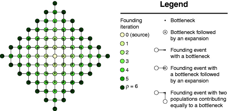
Model of a two-dimensional range expansion with radius ρ = 6. A founding iteration refers to the number of founding events experienced by a population. The source population experiences zero founding events and is at founding iteration zero. Populations founded by the source are at founding iteration 1 because they experience a single founding event. Populations that have experienced exactly k founding events are at founding iteration k. A model with radius ρ has populations at founding iteration ρ and does not have any populations at founding iteration greater than ρ.

Table 1.

Range Expansion Scenarios.

Scenario	Direction of Expansion	Lineages Permitted to Move from Sampled to Unsampled Populations Backward in Time	Migration after Founding	Figure
1	Northeast	No	No	2
2	North	Yes	No	3
3	Northeast	Yes	Yes	5
4	North	Yes	Yes	6
5	North	No	No	7
6	North	Yes	No	8

Using MS (Hudson 2002), we simulated data under two main scenarios, each of which used per-generation per-base mutation and recombination rates of 2.5 × 10⁻⁹, and we set τ_D = 400, N = 500, N_b = 100, L_b = 5, and ρ = 40. For each scenario, we produced 1,000 replicate datasets (figs. 2 and 3), sampling 20 chromosomes of length 100 kilobases per sampled population in each replicate. We calculated mean F_ST between each distinct pair of populations by applying equation 5.3 of Weir (1996) to all loci in all 1,000 replicates that were polymorphic in the full set of sampled populations; polymorphic loci were all bi-allelic. Note that although a coalescent model need only trace lineages from sampled populations, in some of our scenarios, sampled lineages are permitted to migrate in and out of unsampled populations, and we therefore included these unsampled populations in our simulations.

Fig. 2.

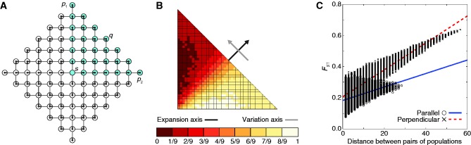
A range expansion model in which geographic sampling occurs in the upper right quadrant of the set of populations along a northeasterly expansion axis. The expansion model follows figure 1. (A) Schematic of the model, with sampled populations shown in blue (radius ρ = 6). (B) PC map (based on a model with radius ρ = 40) in which the value for each population is that population’s value in the first PC (scaled to lie between 0 and 1). (C) Genetic distance, measured by F_ST, between pairs of populations as a function of their Euclidean distance (based on a model with radius ρ = 40). A population pair is parallel to the axis of expansion if the line segment connecting the pair is perpendicular to the line segment connecting p₁ and p₂. A population pair is perpendicular to the axis of expansion if the line segment connecting the pair is parallel to the line segment connecting p₁ and p₂.

Fig. 3.

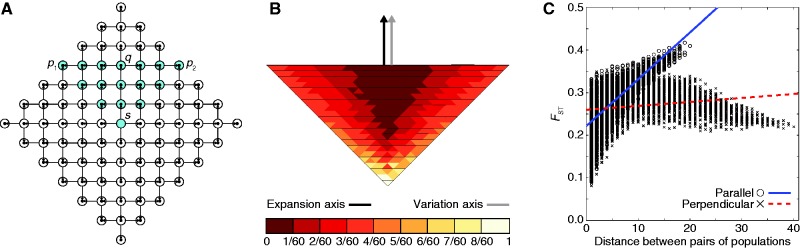
A range expansion model in which geographic sampling occurs along a northerly expansion axis. The expansion model follows figure 1. (A) Schematic of the model, with sampled populations shown in blue (radius ρ = 6). (B) PC map (based on a model with radius ρ = 40) in which the value for each population is that population’s value in the first PC (scaled to lie between 0 and 1). (C) Genetic distance, measured by F_ST, between pairs of populations as a function of their Euclidean distance (based on a model with radius ρ = 40). A population pair is parallel to the axis of expansion if the line segment connecting the pair is parallel to the line segment connecting s and q. A population pair is perpendicular to the axis of expansion if the line segment connecting the pair is perpendicular to the line segment connecting s and q.

PCA

To apply PCA to the simulated data, we generated a matrix of allele frequencies from all polymorphic loci obtained from all 1,000 replicate datasets, in which each row represents a population, each column represents a locus, and each entry represents the frequency of one of the two alleles in a particular population at a particular locus. From this matrix, we centered each column about the mean of the column (Patterson et al. 2006). Using the transformed matrix, we constructed a K × K interpopulation covariance matrix, where K is the number of sampled populations (K = 861 for our first scheme and K = 441 for our second scheme), and the entry for a pair of populations represents the sample covariance of the mean-centered allele frequencies for the population pair (Patterson et al. 2006). Note that our covariance matrix considers population-based rather than individual-based data, unlike in some studies (e.g., Patterson et al. 2006; François et al. 2010).

We applied PCA to the covariance matrix (Patterson et al. 2006) and extracted the first PC. Each PC is associated with a “fraction of variation explained,” a number that describes the variability along the dimension for that PC as a fraction of the total variability in the full multidimensional dataset. The first PC is the dimension that explains the largest fraction of variation in the sample, so that if the data are summarized in a single dimension, values of the first PC are more informative about the structure of relationships among individuals than are values of higher PCs. Using the first PC, we created a PC map of the set of populations by plotting the value, at each population’s geographic location, of the first PC for the population. Identical parameter values were used for both scenarios 1 and 2 and all 1,000 replicates within a given scenario, except that a different set of populations was sampled for scenario 1 compared with scenario 2.

For each scenario, we required a single direction that could be described as the “axis of expansion.” In two dimensions, unless the model is essentially a one-dimensional model with no migration along the other dimension, this choice is not simple. Most studies have not provided a formal definition of the axis of expansion, and, like us, have incorporated expansion occurring in two dimensions from a single starting point. We interpret as the “axis of expansion” the direction of the resultant vector, considering all vectors with a sampled population at the head and the source population at the tail. This direction takes an average of all directions in which expansion is occurring. Using our definition, the axis of expansion for scenario 1 lies at a 45° angle from the x axis of the grid and the axis of expansion for scenario 2 lies at a 90° angle.

Similarly, a choice must be made for the axis of variation in a PC map. We define as the axis of greatest variation in a PC map the axis that connects the locations with the lowest values of the PC to the locations with the highest values.

Results

PCA Maps

Our first scenario (scenario 1) considers populations sampled from the upper right quadrant of the model (fig. 2A). Under this geographic sampling scheme, the PC map displays a gradient of values for the first PC that is perpendicular to the northeasterly axis of expansion (fig. 2B). Defining two populations for which the line segment connecting them is perpendicular to the axis of expansion as a perpendicular pair, and defining two populations connected by a line segment parallel to the axis of expansion as a parallel pair, genetic distance increases faster with geographic distance between perpendicular pairs of populations than it does between parallel pairs (fig. 2C). These results recapitulate the findings of François et al. (2010), in which the axis of greatest variation is perpendicular to the axis of expansion and in which genetic distance increases faster with geographic distance between perpendicular pairs than it does between populations that are parallel to the axis of expansion.

Figure 3 considers a scenario in which populations are sampled in a triangular orientation similar to that of figure 2, except that the axis of expansion in the sampled populations is northerly rather than northeasterly (scenario 2, fig. 3A). Under this geographic sampling scheme, in contrast to the perpendicular gradient observed in figure 2B, the PC map displays a gradient of values for the first PC that is parallel to the northerly axis of expansion (fig. 3B). Unlike in figure 2C, genetic distance increases faster with geographic distance between parallel pairs of populations than it does between perpendicular pairs (fig. 3C).

Coalescence Times and the Axis of Expansion

The patterns observed in figure 3 are quite distinct from those in figure 2, although the range expansion model is identical. The difference stems from the geographic sampling scheme. Under the first scheme (fig. 2), sampling occurs along the northeasterly axis of expansion and supports the view of François et al. (2010) that the first PC can be perpendicular to the axis of expansion. In contrast, under the second scheme (fig. 3), sampling occurs along the northerly axis of expansion and supports the view of Menozzi et al. (1978) that the first PC is parallel to the axis of expansion.

The observed patterns under these two geographic sampling schemes can be explained using the properties of mean pairwise coalescence times. We first recall that for a given set of populations, F_ST = 1 − [T_W]/[T], where [T_W] is the expected coalescence time for a pair of lineages randomly sampled from the same population, averaging across populations, and [T] is the expected coalescence time for two lineages randomly sampled from any two among the set of populations, same or different (Slatkin 1991). For a pair of populations, [T] = ([T_W] + [T_B])/2, where [T_B] is the expected coalescence time for two lineages sampled from distinct populations, so that F_ST can be written ([T_B] − [T_W])/([T_B] + [T_W]).

Using a coalescent-based model with two unstructured populations, McVean (2009) showed that for a pair of populations, the fraction of total variation explained by the first PC is equal to F_ST. Because the first PC by definition is the direction that maximizes the proportion of genetic variation explained, the work of McVean (2009) suggests that identifying the direction of greatest F_ST can identify the orientation of the first PC. Consider populations p₁ and p₂ in figure 2 under scenario 1. A population pair is parallel to the axis of expansion if the line segment connecting the pair is perpendicular to the line segment connecting p₁ and p₂. Populations p₁ and p₂ have an interpopulation expected coalescence time that is at least as large as that of every other pair of sampled populations because lineages sampled from the pair (p₁, p₂) cannot coalesce more recently than τ_D generations in the past. Additionally, because they have experienced at least as many bottlenecks as every other population, p₁ and p₂ each have identical intrapopulation expected coalescence times smaller than or equal to those of any other sampled population. Because among all population pairs, the pair (p₁, p₂) simultaneously maximizes the mean interpopulation coalescence time [T_B] and minimizes the mean intrapopulation coalescence time [T_W], it follows that these two populations have the largest pairwise F_ST. Now consider two populations x and y that represent a perpendicular pair and that are geographically close to p₁ and p₂, respectively. Because of their geographic proximity, population x shares a similar history to p₁ and population y shares a similar history to p₂. As pairwise F_ST is high for the perpendicular pair (p₁, p₂), it is also likely to be high for the perpendicular pair (x, y). Therefore, by this argument, because many perpendicular pairs have high F_ST, the first PC, and hence the axis of greatest variation, is perpendicular to the axis of expansion. The prediction that F_ST is large for (p₁, p₂) is reflected in figure 4A, in which F_ST between p₁ and p₂ (F_ST = 0.629) is greater than F_ST between parallel pairs of populations (e.g., F_ST = 0.261 between q and s). Additionally, figure 2C shows that there are many geographically distant high-F_ST perpendicular pairs and many geographically distant low-F_ST parallel pairs, suggesting greater variation perpendicular rather than parallel to the axis of expansion.

Fig. 4.

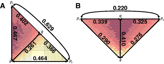
Mean F_ST values across replicate simulations for select pairs of populations under different geographic sampling scenarios. (A) Northeasterly axis of expansion (fig. 2). (B) Northerly axis of expansion (fig. 3).

Similarly, consider population q and the source population s in figure 3A under scenario 2. A population pair is parallel to the axis of expansion if the line segment connecting the pair is parallel to the line segment connecting q and s. Population q has an intrapopulation expected coalescence time that is smaller than that of any other sampled population, as all of its lineages trace backward in time through a single series of founding events, and lineages cannot follow different paths at population founding events. Also, two lineages sampled from the pair (q, s) cannot coalesce more recently than τ_D generations in the past, whereas two lineages sampled from the pair (p, q), where p ≠ s, can coalesce more recently than τ_D. Hence, q and s have an interpopulation expected coalescence time that is larger than that of (p, q), for all p ≠ s. Because among all population pairs, the pair (q, s) maximizes the mean interpopulation coalescence time [T_B] and minimizes the mean intrapopulation coalescence time [T_W], it follows that (q, s) has the largest pairwise F_ST. Now consider two populations x and y that represent a parallel pair and that are geographically close to q and s, respectively. Because of their geographic proximity, population x shares a similar history to q, and y shares a similar history to s. As pairwise F_ST is high for the parallel pair (q, s), it is also likely to be high for the parallel pair (x, y). Therefore, through an argument similar to that used for scenario 1, the first PC, and hence the axis of greatest variation, is parallel rather than perpendicular to the axis of expansion. The prediction that F_ST is large for (q, s) is reflected in figure 4B, in which F_ST between q and s (F_ST = 0.410) is greater than F_ST between perpendicular pairs of populations (e.g., F_ST = 0.220 between p₁ and p₂, F_ST = 0.325 between q and p₂, and F_ST = 0.339 between p₁ and q). Additionally, figure 3C shows that there are many geographically distant high-F_ST parallel pairs and many geographically distant low-F_ST perpendicular pairs, suggesting greater variation parallel rather than perpendicular to the axis of expansion.

Additional Model Features

Our initial pair of scenarios was designed to illustrate two cases that differ only in one feature—the orientation of the sampling with respect to the lattice of populations, and hence, the axis of expansion—and that produced different orientations for the gradient of the first PC. In this section, to investigate the robustness of the initial results, we examine the similarity of the PC patterns generated under three types of modified scenarios to those observed in the initial scenarios.

Migration

First, we introduced migration between pairs of neighboring populations such that after a population is founded, it is permitted to send migrants to extant neighbors to its immediate north, south, east, and west, each at rate M = 4Nm, where m is a per-generation migration rate and N is the population size. We investigated migration rates of M = 4, 40, and 400 for both sampling schemes.

Figure 5 provides results for the first sampling scheme (northeasterly expansion), with the addition of migration between neighboring populations after the initial founding events (scenario 3). For all three migration rates, the PC map displays a gradient of values for the first PC that is perpendicular to the northeasterly axis of expansion (fig. 5B, D, and F). In addition, genetic distance increases faster with geographic distance between perpendicular pairs of populations than it does between parallel pairs (fig. 5C, E, and G). As the migration rate increases, the rate of increase in genetic distance with geographic distance decreases—a consequence of lineages from distant populations having a higher chance of coalescing more recently when migration is more frequent. When the migration rate is high (e.g., M = 400), the high level of gene flow between populations largely obscures the history of the range expansion; the model then becomes similar to an isolation-by-distance model, in which the gradient in the PC map can provide little information about an expansion (Novembre and Stephens 2008). Consider sampling a single lineage each from populations s, q, p₁, and p₂ in figure 5A. Owing to the geometry of the habitat, on average, the time that it takes for a pair of lineages, one sampled from q and the other from s, to reside in the same population (and hence, to have the opportunity to coalesce) is shorter than the corresponding time for a pair of lineages, one sampled from p₁ and the other from p₂. Hence, the pair (q, s) has a smaller interpopulation expected coalescence time than does (p₁, p₂). Even when migration is large enough so that the initial founding bottlenecks have relatively little influence on intrapopulation coalescence times, F_ST between (p₁, p₂) is larger than F_ST between (q, s). As the patterns observed in figure 5 are generally similar to those observed in figure 2, these results indicate that the observations in figure 2 for the first sampling scenario are largely robust to the inclusion of migration between pairs of populations.

Fig. 5.

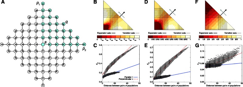
A range expansion model in which geographic sampling occurs in the upper right quadrant of the set of populations along a northeasterly expansion axis, with migration allowed after founding events. The expansion model follows figure 1. After populations are founded, they are permitted to exchange migrants with neighboring populations to their north, south, east, and west at scaled rate M = 4Nm in each direction, where m is the per-generation migration rate and N is the population size. (A) Schematic of the model, with sampled populations shown in blue (radius ρ = 6). (B, D, F) PC map (based on a model with radius ρ = 40) in which the value for each population is that population’s value in the first PC (scaled to lie between 0 and 1) for migration rates of M = 4, 40, and 400, respectively. (C, E, G) Genetic distance, measured by F_ST, between pairs of populations as a function of their Euclidean distance (based on a model with radius ρ = 40) for migration rates M = 4, 40, and 400, respectively. A population pair is parallel to the axis of expansion if the line segment connecting the pair is perpendicular to the line segment connecting p₁ and p₂. A population pair is perpendicular to the axis of expansion if the line segment connecting the pair is parallel to the line segment connecting p₁ and p₂.

Figure 6 displays results for the second sampling scheme (northerly expansion), with the addition of migration between neighboring populations after the initial founding events (scenario 4). For low (M = 4) and moderate (M = 40) migration rates, the PC map displays a gradient of values for the first PC that is parallel to the northerly axis of expansion (fig. 6B and D). Genetic distance increases faster with geographic distance between parallel pairs of populations than it does between perpendicular pairs (fig. 6C and E). When considering a high (M = 400) migration rate, however, an opposite pattern is observed in which the PC map displays a gradient of values for the first PC that is perpendicular, rather than parallel, to the northerly axis of expansion (fig. 6F). The gradient is subtle, as little observable difference exists in the speed with which genetic distance increases with geographic distance between parallel and perpendicular pairs of populations (fig. 6G). Consider sampling a single lineage each from populations s, q, p₁, and p₂ in figure 6A. As in figure 5A, the geographic distance along the lattice between populations q and s is half that between p₁ and p₂, and a smaller interpopulation mean coalescence time might therefore be expected for (q, s) than for (p₁, p₂). However, unlike in figure 5A, in which (q, s) has half the distance of (p₁, p₂) separately in both the horizontal and vertical dimensions, in figure 6A, the distance between q and s lies only in the vertical direction, and the distance between p₁ and p₂ lies only in the horizontal direction. When the migration rate is low, coalescence times are likely to be similar to those in figure 3, in which (q, s) trace their most recent common ancestor to the period prior to any range expansion from s, and have a larger coalescence time than do (p₁, p₂), which can coalesce in a more recent time period. As the migration rate increases, however, so that lineages currently in s might have entered the population through recent migration, it becomes increasingly likely that (q, s) trace their most recent common ancestor to the period subsequent to the initial range expansion outward from s. It is then not unreasonable that (q, s) and (p₁, p₂) might have similar coalescence times, so that F_ST between (p₁, p₂) could be similar to F_ST between (q, s). Thus, while the pattern in the scenario of figure 3 dissipates when the amount of migration after the initial range expansion is large, it is largely robust to smaller and intermediate levels of migration.

Fig. 6.

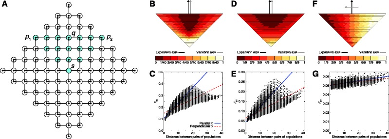
A range expansion model in which geographic sampling occurs along a northerly expansion axis, with migration allowed after founding events. The expansion model follows figure 1. After populations are founded, they are permitted to exchange migrants with neighboring populations to their north, south, east, and west at scaled rate M = 4Nm in each direction, where m is the per-generation migration rate and N is the population size. (A) Schematic of the model, with sampled populations shown in blue (radius ρ = 6). (B, D, F) PC map (based on a model with radius ρ = 40) in which the value for each population is that population’s value in the first PC (scaled to lie between 0 and 1) for migration rates of M = 4, 40, and 400, respectively. (C, E, G) Genetic distance, measured by F_ST, between pairs of populations as a function of their Euclidean distance (based on a model with radius ρ = 40) for migration rates M = 4, 40, and 400, respectively. A population pair is parallel to the axis of expansion if the line segment connecting the pair is parallel to the line segment connecting s and q. A population pair is perpendicular to the axis of expansion if the line segment connecting the pair is perpendicular to the line segment connecting s and q.

Connectivity

The northerly expansion scenario of figure 3 has the perhaps nonintuitive property that lineages in sampled populations can trace their ancestry to unsampled populations. Therefore, in a second experiment, we examined the effect of disallowing genetic contributions from unsampled populations to sampled populations. This issue affects only the northerly expansion scenario of figure 3, as the northeasterly expansion scenario of figure 2 does not allow lineages in sampled populations to have ancestry in unsampled populations. We modified the initial model solely by eliminating founding events with origins in unsampled populations (scenario 5, fig. 7A). Under this scenario, the PC map displays a gradient of values for the first PC that is parallel to the northerly axis of expansion (fig. 7B). In addition, genetic distance increases faster with geographic distance between parallel pairs of populations than it does between perpendicular pairs (fig. 7C). These results are quite similar to those observed in figure 3, suggesting that coalescence of lineages in unsampled populations was not a major contributor to the observation of a parallel axis of variation in figure 3.

Fig. 7.

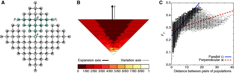
A range expansion model in which geographic sampling occurs along a northerly expansion axis, with no gene flow allowed from an unsampled to a sampled population. The expansion model follows figure 1. (A) Schematic of the model, with sampled populations shown in blue (radius ρ = 6). (B) PC map (based on a model with radius ρ = 40) in which the value for each population is that population’s value in the first PC (scaled to lie between 0 and 1). (C) Genetic distance, measured by F_ST, between pairs of populations as a function of their Euclidean distance (based on a model with radius ρ = 40). A population pair is parallel to the axis of expansion if the line segment connecting the pair is parallel to the line segment connecting s and q. A population pair is perpendicular to the axis of expansion if the line segment connecting the pair is perpendicular to the line segment connecting s and q.

Shape of Sampled Region

It is also possible that the parallel axis of variation observed in figure 3 might have resulted from sampling in a triangular rather than a rectangular region. We therefore explored the influence of the geometry of the sampled region by considering a square, rather than a triangular, sampling geometry (scenario 6, fig. 8A). Under this square sampling geometry for a northerly expansion scenario, the PC map displays a gradient of values for the first PC that is parallel to the northerly axis of expansion (fig. 8B). In addition, genetic distance increases faster with geographic distance between parallel pairs of populations than it does between perpendicular pairs (fig. 8C). As these patterns are similar to those observed under the triangular sampling geometry (fig. 3), the results of figure 8 suggest that the patterns observed for scenario 2 are not an artifact of the shape of the sampled region.

Fig. 8.

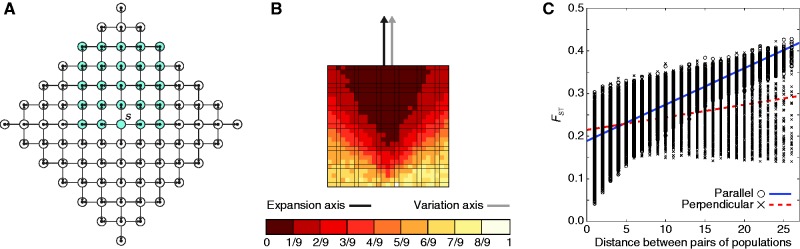
A range expansion model in which geographic sampling occurs along the northerly expansion axis, with a square sampling region. The expansion model follows figure 1. (A) Schematic of the model, with sampled populations shown in blue using a square sampling region (radius ρ = 6 and 5 × 5 sampling grid). (B) PC map (based on a model with radius ρ = 40 and 27 × 27 sampling grid) in which the value for each population is that population’s value in the first PC (scaled to lie between 0 and 1). (C) Genetic distance, measured by F_ST, between pairs of populations as a function of their Euclidean distance (based on a model with radius ρ = 40 and 27 × 27 sampling grid). A population pair is parallel to the axis of expansion if the line segment connecting the pair is parallel to the line segment connecting s and q. A population pair is perpendicular to the axis of expansion if the line segment connecting the pair is perpendicular to the line segment connecting s and q.

Discussion

By considering scenarios with different sampling schemes, we have shown that depending on the geographic sampling used under the same range expansion model, the axis of greatest variation in PCA can be either perpendicular or parallel to the axis of expansion. Our results have pointed to a set of fundamental population-genetic quantities—intra- and interpopulation mean coalescence times—that enable a range expansion model to produce different directions for gradients in PC maps. The results illustrate both the complexity of interpreting PCA results in terms of evolutionary models (e.g., Novembre and Stephens 2008), as well as the utility of a theoretical approach (e.g., McVean 2009) in disentangling possible scenarios. We expect that use of coalescence times can potentially assist in understanding PCA patterns in more complex models, such as spatially continuous models, which are not constrained by a population lattice.

François et al. (2010) used “sectors” to explain how an axis perpendicular to the axis of expansion could potentially yield greater variation than an axis parallel to the axis of expansion. In terms of coalescence times, the production of sectors with different allelic profiles traces to the potentially larger interpopulation mean coalescence times for pairs of populations along a perpendicular axis than along a parallel axis. However, different patterns of high-frequency alleles in different sectors might not always provide a complete explanation for patterns in the first PC, as it is possible for the parallel axis connecting the source to a population at the edge of the expansion to produce a greater interpopulation mean coalescence time than a perpendicular axis that connects different sectors. The relatively large interpopulation coalescence times between populations representing different sectors, depending on the sampling scheme, might be smaller than the interpopulation coalescence times between the source and populations at the edge of the expansion. Thus, we suggest that in addition to considering the standpoint of sectors, examining mean coalescence times can provide an informative basis for evaluating the factors that give rise to spatial patterns in the PCs.

The models considered here, as well as those of Rendine et al. (1986) and François et al. (2010), have focused on situations in which range expansions actually occurred (see also Arenas et al. 2012). Under quite simple model formulations, we have found that if a range expansion did occur, because both parallel and perpendicular axes in the first PC are possible under the model, it is difficult to infer the direction of the expansion from PC maps alone. Novembre and Stephens (2008) further showed that gradients in PC maps can be observed under models in which no expansion has occurred. Therefore, individual PC gradients do not uniquely identify the properties of a range expansion, as the same gradient in a PC could potentially represent an expansion parallel to the gradient, an expansion perpendicular to the gradient, or no expansion at all. Our results support the contention of Novembre and Stephens (2008) that caution is warranted in interpreting the history underlying any given PC gradient, and that consideration of two or more PCs jointly with other analyses (e.g., Lao et al. 2008; Novembre et al. 2008; Price et al. 2009; Bryc et al. 2010; Wang et al. 2010, 2012; Xing et al. 2010; Henn et al. 2011; Metspalu et al. 2011; Pagani et al. 2012) is desirable for providing further insight into the processes that underlie patterns in PCA.

References

- Arenas M, François O, Currat M, Ray N, Excoffier L. Influence of admixture and paleolithic range contractions on current European diversity gradients. Mol Biol Evol. 2012 doi: 10.1093/molbev/mss203. Advance Access published August 25, 2012, doi:10.1093/molbev/mss203. [DOI] [PubMed] [Google Scholar]
- Bryc K, Auton A, Nelson MR, et al. (11 co-authors) Genome-wide patterns of population structure and admixture in West Africans and African Americans. Proc Natl Acad Sci U S A. 2010;107:786–791. doi: 10.1073/pnas.0909559107. [DOI] [PMC free article] [PubMed] [Google Scholar]
- Cavalli-Sforza LL, Menozzi P, Piazza A. The history and geography of human genes. Princeton (NJ): Princeton University Press; 1994. [Google Scholar]
- Edmonds CA, Lillie AS, Cavalli-Sforza LL. Mutations arising in the wave front of an expanding population. Proc Natl Acad Sci U S A. 2004;101:975–979. doi: 10.1073/pnas.0308064100. [DOI] [PMC free article] [PubMed] [Google Scholar]
- Excoffier L, Ray N. Surfing during population expansions promotes genetic revolutions and structuration. Trends Ecol Evol. 2008;23:347–351. doi: 10.1016/j.tree.2008.04.004. [DOI] [PubMed] [Google Scholar]
- François O, Currat M, Ray N, Han E, Excoffier L, Novembre J. Principal component analysis under population genetic models of range expansion and admixture. Mol Biol Evol. 2010;27:1257–1268. doi: 10.1093/molbev/msq010. [DOI] [PubMed] [Google Scholar]
- Hallatschek O, Hersen P, Ramanathan S, Nelson DR. Genetic drift at expanding frontiers promotes gene segregation. Proc Natl Acad Sci U S A. 2007;104:19926–19930. doi: 10.1073/pnas.0710150104. [DOI] [PMC free article] [PubMed] [Google Scholar]
- Hallatschek O, Nelson DR. Gene surfing in expanding populations. Theor Popul Biol. 2008;73:158–170. doi: 10.1016/j.tpb.2007.08.008. [DOI] [PubMed] [Google Scholar]
- Henn BM, Gignoux CR, Jobin M, et al. (19 co-authors) Hunter-gatherer genomic diversity suggests a southern African origin for modern humans. Proc Natl Acad Sci U S A. 2011;108:5154–5162. doi: 10.1073/pnas.1017511108. [DOI] [PMC free article] [PubMed] [Google Scholar]
- Hudson RR. Generating samples under a Wright-Fisher neutral model. Bioinformatics. 2002;18:337–338. doi: 10.1093/bioinformatics/18.2.337. [DOI] [PubMed] [Google Scholar]
- Klopfstein S, Currat M, Excoffier L. The fate of mutations surfing on the wave of a range expansion. Mol Biol Evol. 2006;23:482–490. doi: 10.1093/molbev/msj057. [DOI] [PubMed] [Google Scholar]
- Lao O, Lu TT, Nothnagel M, et al. (33 co-authors) Correlation between genetic and geographic structure in Europe. Curr Biol. 2008;18:1241–1248. doi: 10.1016/j.cub.2008.07.049. [DOI] [PubMed] [Google Scholar]
- McVean G. A genealogical interpretation of principal components analysis. PLoS Genet. 2009;5:e1000686. doi: 10.1371/journal.pgen.1000686. [DOI] [PMC free article] [PubMed] [Google Scholar]
- Menozzi P, Piazza A, Cavalli-Sforza L. Synthetic maps of human gene frequencies in Europeans. Science. 1978;201:786–792. doi: 10.1126/science.356262. [DOI] [PubMed] [Google Scholar]
- Metspalu M, Gallego Romero I, Yunusbayev B, et al. (15 co-authors) Shared and unique components of human population structure and genome-wide signals of positive selection in south Asia. Am J Hum Genet. 2011;89:731–744. doi: 10.1016/j.ajhg.2011.11.010. [DOI] [PMC free article] [PubMed] [Google Scholar]
- Novembre J, Johnson T, Bryc K, et al. (12 co-authors) Genes mirror geography in Europe. Nature. 2008;456:98–101. doi: 10.1038/nature07331. [DOI] [PMC free article] [PubMed] [Google Scholar]
- Novembre J, Stephens M. Interpreting principal component analyses of spatial population genetic variation. Nat Genet. 2008;40:646–649. doi: 10.1038/ng.139. [DOI] [PMC free article] [PubMed] [Google Scholar]
- Pagani L, Kivisild T, Tarekegn A, et al. (14 co-authors) Ethiopian genetic diversity reveals linguistic stratification and complex influences on the Ethiopian gene pool. Am J Hum Genet. 2012;91:83–96. doi: 10.1016/j.ajhg.2012.05.015. [DOI] [PMC free article] [PubMed] [Google Scholar]
- Patterson N, Price AL, Reich D. Population structure and eigenanalysis. PLoS Genet. 2006;2:2074–2093. doi: 10.1371/journal.pgen.0020190. [DOI] [PMC free article] [PubMed] [Google Scholar]
- Price AL, Helgason A, Palsson S, Stefansson H, St Clair D, Andreassen OA, Reich D, Kong A, Stefansson K. The impact of divergence time on the nature of population structure: an example from Iceland. PLoS Genet. 2009;5:e1000505. doi: 10.1371/journal.pgen.1000505. [DOI] [PMC free article] [PubMed] [Google Scholar]
- Rendine S, Piazza A, Cavalli-Sforza LL. Simulation and separation by principal components of multiple demic expansions in Europe. Am Nat. 1986;128:681–706. [Google Scholar]
- Slatkin M. Inbreeding coefficients and coalescence times. Genet Res. 1991;58:167–175. doi: 10.1017/s0016672300029827. [DOI] [PubMed] [Google Scholar]
- Wang C, Szpiech ZA, Degnan JH, Jakobsson M, Pemberton TJ, Hardy JA, Singleton AB, Rosenberg NA. Comparing spatial maps of human population–genetic variation using Procrustes analysis. Stat Appl Genet Mol Biol. 2010;9:13. doi: 10.2202/1544-6115.1493. [DOI] [PMC free article] [PubMed] [Google Scholar]
- Wang C, Zöllner S, Rosenberg NA. A quantitative comparison of the similarity between genes and geography in worldwide human populations. PLoS Genet. 2012;8:e1002886. doi: 10.1371/journal.pgen.1002886. [DOI] [PMC free article] [PubMed] [Google Scholar]
- Weir BS. Genetic data analysis II. Sunderland (MA): Sinauer Associates; 1996. [Google Scholar]
- Xing J, Watkins WS, Shlien A, et al. (13 co-authors) Toward a more uniform sampling of human genetic diversity: a survey of worldwide populations by high-density genotyping. Genomics. 2010;96:199–210. doi: 10.1016/j.ygeno.2010.07.004. [DOI] [PMC free article] [PubMed] [Google Scholar]