Joint entropy of continuously differentiable ultrasonic waveforms

Abstract

This study is based on an extension of the concept of joint entropy of two random variables to continuous functions, such as backscattered ultrasound. For two continuous random variables, X and Y, the joint probability density $p(x,y)$ is ordinarily a continuous function of x and y that takes on values in a two dimensional region of the real plane. However, in the case where $X=f(t)$ and $Y=g(t)$ are both continuously differentiable functions, X and Y are concentrated exclusively on a curve, $\gamma (t)=(f(t),g(t))$, in the $x,y$ plane. This concentration can only be represented using a mathematically “singular” object such as a (Schwartz) distribution. Its use for imaging requires a coarse-graining operation, which is described in this study. Subsequently, removal of the coarse-graining parameter is accomplished using the ergodic theorem. The resulting expression for joint entropy is applied to several data sets, showing the utility of the concept for both materials characterization and detection of targeted liquid nanoparticle ultrasonic contrast agents. In all cases, the sensitivity of these techniques matches or exceeds, sometimes by a factor of two, that demonstrated in previous studies that employed signal energy or alternate entropic quantities.

INTRODUCTION

Previous studies have demonstrated the utility of several different entropies for detection of subresolution backscattering structures in both materials characterization and medical ultrasonics in situations where other approaches fail. These include detection of unresolvable near-surface defects,1, 2, 3, 4, 5 diffuse accumulation of subresolution-sized nanoparticle-based ultrasound contrast agents,6, 7, 8, 9, 10 characterization of smooth muscle pathologies,11, 12, 13 and monitoring of ultrasonically induced temperature rise in tissue.14

In the first of these studies, entropy images were applied to detect defects in advanced aerospace materials.1 In particular, detection and imaging of “near-surface” defects in graphite-epoxy composite plates was accomplished using a 5 MHz center frequency transducer.1, 2, 3, 4, 5 In this application, it is not possible to separate the front wall echo from the defect reflection. This presents a significant challenge to conventional approaches for defect detection and imaging. In fact, the case presented in the following text is nearly impossible to discern using the traditional approach. However, the joint entropy image permits visualization of the defect, its boundary, and certain substructures contained in the defect that were not visible to conventional detection methods or even the previously published entropic images.

The bulk of our investigations have focused on medical imaging. These studies have demonstrated the utility of several different entropies for detection of subresolution structures of backscattering tissue: e.g., targeted accumulation of weakly scattering perfluorocarbon nanoparticles in tissues in vivo, and pathological changes in smooth muscle structure arising from muscular dystrophy. These results have been obtained in a variety of animal disease models and in patients as shown in Table TABLE I.. Several features common to these studies deserve special emphasis at the outset:

• (a)Studies have been executed using several different imaging systems (Philips HDI 5000, Philips IE33, Vevo 660, Ardent Spark) with transducer arrays covering a frequency range from 2–34 MHz.
• (b)In all cases but one,11 the entropic analysis demonstrated greater sensitivity than did signal energy to subresolution features of scattering architecture. In the exceptional case,11 sensitivities were essentially equivalent.
• (c)The most recent version of entropy published8, 15 is amenable to real-time implementation.
• (d)All results pertaining to detection of targeted nanoparticles were obtained without use of hand-drawn regions of interest. In fact, the entire analysis chain from raw data to image construction to image-based sensitivity assessment was automated and thus objective.
• (e)Image subtraction has not been required to detect changes in scattering architecture.

TABLE I.

Summary of studies based on different entropic signal receivers defined for waveform $y=f(t)$ having density function $w_f(y)$: entropy, $H_f$, Renyi entropy, $I_f(r)$, and its asymptotic limiting form, $I_{f,\infty }$. The joint entropy $H_{f,g}$ is frequently much more sensitive than any of these.

“Entropic” receiver	Heuristic meaning	Scattering structure	Experimental system
$H_f=-{\int }_{f_{\mathit{m}\mathit{i}\mathit{n}}}^{f_{\mathit{m}\mathit{a}\mathit{x}}}{w}_f(y)\log \left[w_f(y)\right]dy$	“Information” contained	Materials characterization,	Graphite/epoxy laminates (Ref. 5)
$H_f=-{\int }_0^1\log \left[{f\prime }_{\uparrow }(t)\right]dt$	“Information” contained in backscattered RF $f(t)$.	Targeted nanoparticles, smooth muscle cells	MDA 435 (Ref. 16), B16
			VX2,MDx mice (Ref. 11)
			Precancer models (Ref. 7)
			Humans (Ref. 12)
$I_f(r)=1/1-r\text{log}{\int }_{f_{\mathit{min}}}^{f_{\mathit{max}}}{w}_f{(y)}^r\mathit{dy}$	“Weighted-information” contained in backscattered RF: $f(t)$ (note: $H_f=I_f(1)$).	Targeted nanoparticles, smooth muscle cells	MDA 435, B16 Precancer models (Ref. 17)
$I_{f,\infty }=\log \left[\left\{t_k\right|f\prime (t_k)=0\}1/\left|f^{″}\left(t_k\right)\right|\right]$	Limiting form of $I_f(r)$ as $r\to 2$. More sensitive than $H_f$, $I_f(r)$.	Targeted nanoparticles,	MDA 435 (Ref. 8), B16 (Ref. 10)
		smooth muscle cells	Humans
			Precancer models (Ref. 15)

All of these points suggest the clinical utility of this approach, which might proceed along lines similar to that employed in Doppler imaging systems, where the conventional B-mode image is color-coded according to the blood cell velocity to present a combined B-mode/velocity image; similarly, a B-mode/entropy image could be made as well.9

All of these investigations required acquisition of thousands of radio frequency (RF) signals, $f(t)$. For each of these captured waveforms, viewed as a sampled version of a differentiable function, the probability density function of values was computed using the digitized values of $f(t)$. Distributions of values (or densities of distributions of values) are typically used for analysis of random variables, and all differentiable functions are, in fact, legitimate random variables. However, in the general case, it is not possible to compute the probability density function of a random variable solely from its values. For example, to determine the probability density function for noise in an amplifier, the noise source must be sampled and the distribution of sampled values subsequently fit to an assumed functional form, e.g., Gaussian or Poisson. In our case, the knowledge that the random variable $f(t)$ is differentiable permits direct computation of its probability density function without the need to assume and fit a model.2, 5, 7 While this can be a mathematically and computationally demanding task, previous applications of this approach to analysis of acoustic signals have repeatedly demonstrated its utility. The present study extends these results by developing joint entropy, which we will denote by $H_{f,g}$, to analyze the same type of data. This approach requires computation of the joint probability density of two (differentiable) functions: $y=f(t)$, representing a segment of backscattered radio frequency ultrasound, and a reference signal, $g(t)$. After carefully deriving a suitable expression for $H_{f,g}$, we show that it provides further improvements in sensitivity over those obtained in previous studies that were based on other entropies.

APPROACH

Our goal is to further improve the ability to detect weak scatterers in strongly scattering environments, as in the case where liquid nanoparticles are targeted to cancer molecular epitopes or in material defects in advanced aerospace materials. Although prior entropy measures have been proposed, we expect the current approach to demonstrate significant enhancement in detection in real-time applications that could be ported to existing imaging systems.

Background

This study is based on an extension of the concept of joint entropy of two random variables to continuous functions, such as backscattered RF, and a reference signal, such as a reflection from a weak reflector. For two continuous random variables, X, Y with joint probability density function $p(x,y)$, the joint entropy is

$$H(X,Y)={\displaystyle {\int }_{-\infty }^{\infty }{\displaystyle {\int }_{-\infty }^{\infty }p(x,y)\hspace{0.17em}\text{log}\hspace{0.17em}p(x,y)dxdy}}.$$ (1)

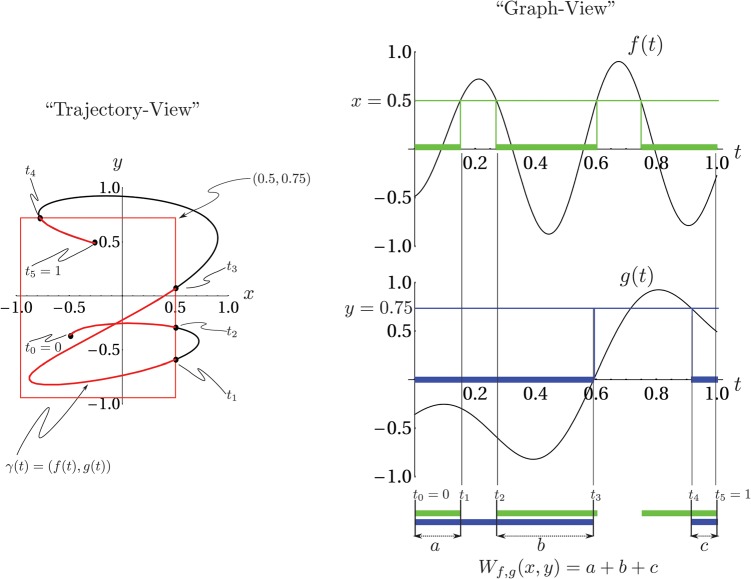
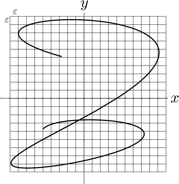
Ordinarily $p(x,y)$ is a continuous function of x and y that takes non-zero values in a two dimensional region of the real plane. However, in the case where $X=f(t)$ and $Y=g(t)$ are both continuously differentiable functions, the random variables X and Y are concentrated exclusively on a curve, $\gamma (t)=(f(t),g(t))$, in the $\mathrm{x,y}$ plane as shown in Fig. 1. Thus the densities of their values cannot be represented using conventional functions as was done in previous studies of only one differentiable random variable.1, 2, 3, 4, 5, 7 Instead, this concentration can only be represented using a mathematically “singular” object like a series of Dirac Delta functions placed on $\gamma (t)$ with infinitesimal spaces in between them. Technically, such an object is not a function; in precise terms, $p(x,y)$ must be represented as a Schwartz distribution.16 Its use for imaging requires that the Schwartz distribution be coarse-grained, i.e., integrated, on a fine grid of small cells as shown in Fig. 2. The outcome of this course-graining, as shown in Appendix B, is the conversion of the probability density (which is a Schwartz distribution) into a bona fide probability distribution function such that the probability of X and Y being in a particular cell, which is the generalization of $p(x,y)$ that we seek, is given by the time that $\gamma (t)$ “spends” in the cell [Eq. B28 in the following text]. This is what we would expect intuitively if we imagined a test particle traversing the curve, $\gamma (t)$, with velocity $v(t)=\sqrt{f\prime {\left(t\right)}^2+g\prime {\left(t\right)}^2}$, and wanted to know the probability of finding it in a particular cell. Having this result, it is possible to extract a well-defined finite component from the coarse-grained version of Eq. 1, which we will denote by $H_{f,g}$, in terms of $f\prime (t)$ and $g\prime (t)$.

Figure 1.

(Color online) Left panel: A plot of the curve $\gamma (t)$ used to visualize the joint cumulative density function, $W(x,y)$, of values of the functions $f(t)$ and $g(t)$. The probability density is non-zero only on the curve $\gamma (t)$ because the random variables $X=f(t)$, $Y=g(t)$are concentrated exclusively on $\gamma (t)$. On the right is an graphical calculation of $W(x,y)$ using the graphs of $f(t)$ and $g(t)$. The exact definition of $W(x,y)$ is given in Eq.B1.

Figure 2.

Uniform partition of the $\mathit{x}\mathit{y}$-plane into $\epsilon \times \epsilon$ cells.

As with the entropies previously investigated, $H_{f,g}$ is applied in a moving window analysis. However, its computation requires two input waveforms. The first, $f(t)$, is exactly the same as in previous investigations. However, choice of the second reference waveform, $g(t)$, constitutes an additional degree of freedom that may be exploited to increase sensitivity of the entropic analysis. Discovery of strategies for identification of the optimum reference waveform is one of the eventual goals of our research. In this study, we present the results of preliminary investigations that indicate a reflection of the imaging system's interrogating pulse from a weak reflector, such as a water-agarose interface, constitutes a good initial guess for the optimum. To summarize our findings:

• (a)$H_{f,g}$ analysis may be applied in the same situations as previous entropies, $H_f$, $I(r)$, $I_{f,\infty }$. In fact, all of the data for this study have been analyzed previously with the use of at least one of these entropies. In this study, we repeat several of these analyses using $H_{f,g}$ images.
• (b)$H_{f,g}$ analysis is amenable to real-time implementation, as was $I_{f,\infty }$ analysis.
• (c)In all cases studied so far, $H_{f,g}$ analysis has proven to be more sensitive than the best previous results obtained by other entropies. For example, preliminary application of this new entropy to the MDA 435 data shown in Figs. 7 and 8 shows a roughly twofold increase in peak confidence ratios.

Figure 7.

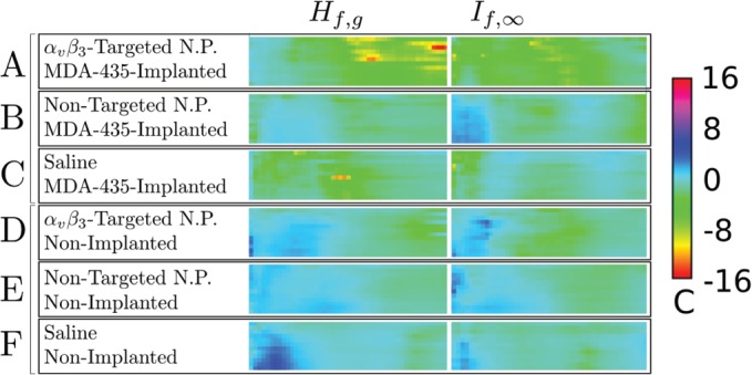
Confidence, c, panels for $\Delta H_{f,g}$ (left column) and $\Delta I_{f,\infty }$ (right column) for all groups used in our study. (A) MDA 435-implanted mice injected with ${\alpha }_v{\beta }_3$-targeted nanoparticles ($N=5$), (B) MDA 435-implanted mice injected with non-targeted nanoparticles ($N=5$), (C) MDA 435-implanted mice injected with saline ($N=5$), (D)–(F), same injections into $N=5$ tumor-free mice. The smoothing spline parameter $S=1.0$ in all cases. A color-to-confidence calibration bar is shown to the right of the confidence panels.

Figure 8.

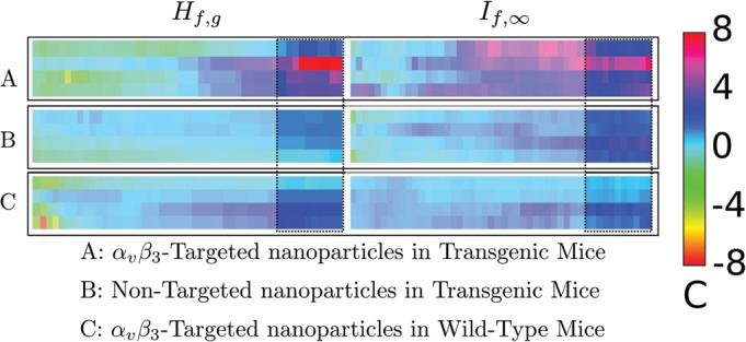
Comparison $\Delta H_{f,g}$ (left) and $\Delta I_{f,\infty }$ (right) for data acquired in a pre-cancer model (Ref. 7) like that shown in Fig. 7. While analysis at all thresholds between 0% and 100% was undertaken, we wish to focus attention on the results obtained between 75% and 100% (results from lower analysis thresholds have been “dimmed” by a translucent overlay). In both cases, a broad region of confidence values above 2 is shown. While the extent of this region is larger in the $\Delta I_{f,\infty }$ confidence panel, the maximum height of the $\Delta H_{f,g}$ confidence panel is more than twice as high (16.0 vs 6.8). A color-to-confidence calibration bar is shown to the right of the confidence panels.

Conventions and calculation

To fix terminology, suppose that we are given two functions, $f(t)$ and $g(t)$, assumed to map $[0,1]$ into $(-1,1)$ (i.e., $\left|\hspace{0.17em}{f}_{\text{max}}\right|$, $\left|f_{\text{min}}\right|$, $\left|g_{\text{max}}\right|$, $\left|g_{\text{min}}\right|$ are all strictly less than one). We are interested in computing the joint entropy,

$$H(f,g)={\displaystyle {\int }_{-1}^1\mathit{d}\mathit{x}}{\displaystyle {\int }_{-1}^1\mathit{d}\mathit{y}}\hspace{0.17em}\hspace{0.17em}w(x,y)\text{log}[w(x,y)],$$ (2)

where $w(x,y)$ is their joint density, defined on the domain $\Omega =(-1,1)\times (-1,1)$. It turns out that for the types of functions $f\left(t\right)$ and $g(t)$ that we will consider (intuitively thought of as “well-behaved”), $w(x,y)$ is not a real-valued function but a (Schwartz) distribution so that Eq. 2 is not well-defined.

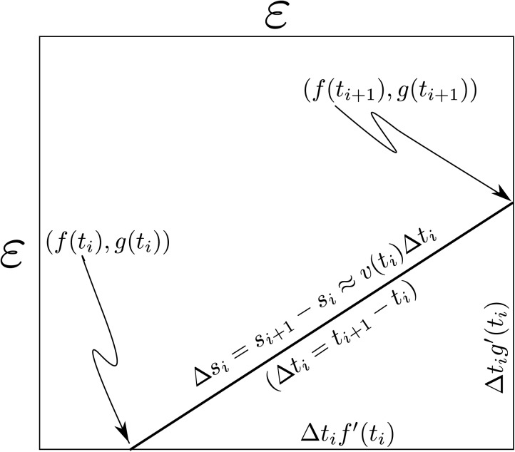
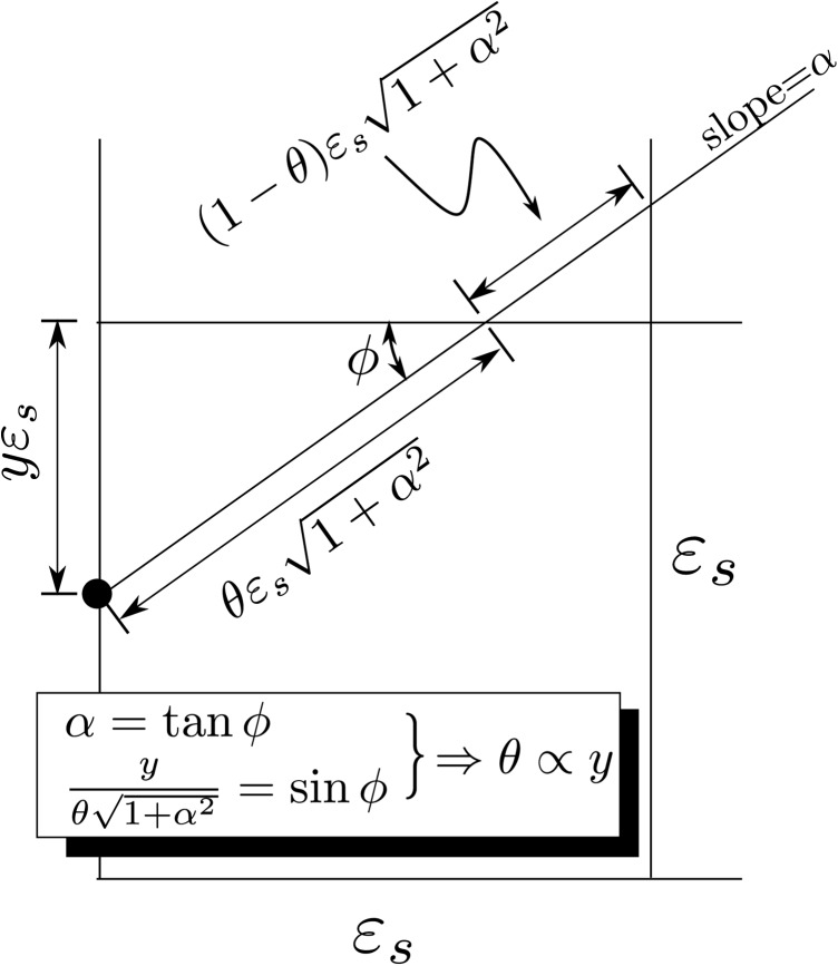
To get around this difficulty, we employ a “coarse-grained” approximation to Eq. 2 obtained, by dividing Ω into $\epsilon \times \epsilon$ cells, where $\epsilon =1\hspace{0.17em}/\hspace{0.17em}N$ as shown in Fig. 2, and integrating $w(x,y)$ over each cell. We denote the $\epsilon \times \epsilon$ cells intersecting $\gamma (t)$ at initial time $t_i$ by $C_i$ and index them by $i=1,\dots ,M$ (M will be discussed later). For subsequent discussion, we define the distance traversed along $\gamma (t)$ when it enters the $i\text{th}$ cell by $s_i$. Figure 9 illustrates our terminology. The final step in the coarse-graining process is replacement of $H(\mathrm{f,g})$ by the quantity $H_{f,g}$ defined by

$$\begin{array}{c}{H}_{f,g}=\underset{ϵ\to 0}{\text{lim}}\left[H^{\Delta }(f,g)-\epsilon \right]\\ =\underset{ϵ\to 0}{\lim }\left[{\displaystyle \sum }_{j,k}{p}^{\Delta }(j,k)\hspace{0.17em}\log \left[p^{\Delta }(j,k)\right]-\epsilon \right],\end{array}$$ (3)

where $p^{\Delta }(j,k)=0$ unless $\gamma (t)$ passes through the $(j,k)\text{th}$ cell, in which case (as mentioned in the preceding text and as we shall show in the following text), $p^{\Delta }(j,k)$ is equal to the time $\gamma (t)$ spends in the $(j,k)\text{th}$ cell.

Figure 9.

A diagram of the computation of time spent by $\gamma (t)$ in an $\epsilon \times \epsilon$ cell in the $\mathit{x}\mathit{y}$ plane.

Our ultimate goal is to obtain an expression for $H_{f,g}$ in terms of $f(t)$ and $g(t)$ because these quantities are experimentally accessible. As is carefully shown in Appendixes A–C, the following relation is true:

$$\begin{array}{c}{H}_{f,g}\equiv -\frac{1}{2}{\displaystyle {\int }_0^{1}dt\hspace{0.17em}\frac{min[|\hspace{0.17em}f\prime (t)\hspace{0.17em}|,|\hspace{0.17em}g\prime (t)\hspace{0.17em}|]}{max[|\hspace{0.17em}f\prime (t)\hspace{0.17em}|,|\hspace{0.17em}g\prime (t)\hspace{0.17em}|]}}\\ -{\displaystyle {\int }_0^{1}dt\hspace{0.17em}\text{log}\left[|\hspace{0.17em}max[|\hspace{0.17em}f\prime (t)\hspace{0.17em}|,|\hspace{0.17em}g\prime (t)\hspace{0.17em}|]\hspace{0.17em}|\right].}\end{array}$$ (4)

It is a remarkable fact that derivation of Eq. 4, which uses the ergodic theorem, also requires the fact that the set of points for which $f\prime (t)/g\prime (t)$ is rational comprises a set of measure zero (in the set of real numbers). Thus the relation is essentially derived in a noncomputable setting. Nevertheless, the end result, Eq. 4, may be evaluated numerically. The full details are provided in the appendixes.

RESULTS

Noise simulation

The effect of noise on the input waveform $f(t)$ is shown in Fig. 3. To produce this plot, Gaussian distributed noise of different amplitude was added to $f(t)=e^{-10{(t-0.4)}^2}\text{sin}(4\pi t)$ and $g(t)=e^{-10{(t-0.4)}^2}\sin (2\pi t)$ (simulations using uniformly distributed noise have also been performed yielding essentially similar results). The range of noise levels spans 20 to 120 dB. At each noise level, 1000 waveforms $f(t)$ and reference waveforms $g(t)$ were created, $H_{f,g}$ computed, and the average $\langle H_{f,g}\rangle$ and standard error computed. Each $\langle H_{f,g}\rangle$ is shown in the plot, with its standard error bar, which in all but one case is too small to see. We notice that for signal-to-noise ratios above 80 dB, it is possible to obtain three-digit agreement with the noise-free answer [which was obtained using a separate mathematica implementation of Eq. 4 that was also used to double check the correctness of our C programming language implementation of the same equation]. However, for signal-to-noise ratios between 40 and 60 dB, which is the relevant range for our experimental data, agreement to at most one or two digits is achievable. This limitation shows that the numerical precision of our composite integrator is more than enough for analysis of experimental data, which always contain noise.

Figure 3.

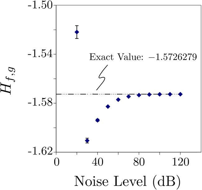
(Color online) Effect noise on the computation of $H_{f,g}$ using Eq. 4. Each data point is the average of $H_{f,g}$ computed from $N=1000$ different waveforms $g(t)=e^{-10{(t-0.4)}^2}\sin (2\pi t)$ to which Gaussian noise has been added. The signal-to-noise ratio simulated ranges from 20 to 120 dB. The reference trace $f(t)=e^{-10{(t-0.4)}^2}\sin (4\pi t)$ did not have noise added. Standard error bars are plotted with each point, most are too small to see on the scale of the plot.

Materials characterization: Defect detection

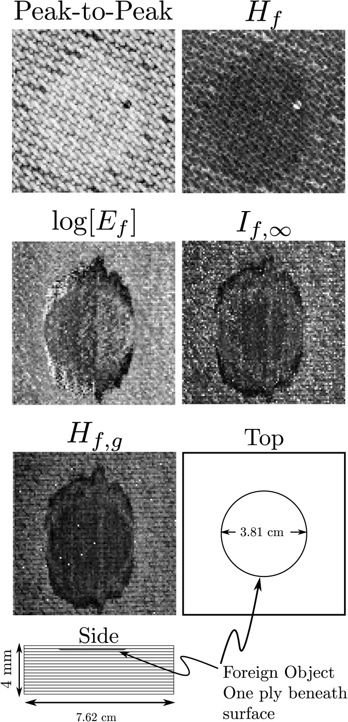
The first application of entropy imaging was to materials characterization;17 in particular, to detection and sizing of near-surface defects in graphite/epoxy aerospace structures.1, 2, 3, 4, 5 Figure 4 shows some previously published (top row)5 and newer results (middle and bottom row) for imaging of a near-surface “resin-rich” defect in a thin (4 mm thick) graphite/epoxy composite. The bottom left corner shows a schematic of the specimen, which was fabricated by removing a 3.81 cm diameter circular section from the second ply prior to fabrication. The specimen was then autoclaved following standard manufacturing practice. This forced excess epoxy into the circular void and created the resin-rich region. During the fabrication procedure, additional resin penetrated the inter-laminar region bordering the circular void. The result is an oval shaped defect centered on the original circular cutout.

Figure 4.

Five different types of images made using RF backscattered from a graphite/epoxy plate with a near-surface defect. Top row contains previously published results (Ref. 5). These were obtained using the full 512-point digitized waveform and without optimal smoothing splines. The next two rows show the results obtained using optimal smoothing splines on a 128-point subset of the full digitized waveform. A schematic of the experimental specimen is shown in the lower left corner of the figure. The $H_{f,g}$ image shows the clearest delineation of defect boundaries.

This specimen was scanned on a 101 × 101 point grid using a 5 MHz broadband transducer with the backscattered RF acquired at 8-bit digital resolution and a 100 MHz sampling rate. The width of the interrogating pulse was therefore far too wide to permit gating of front-wall reflection from that of the defect, which lay within one ply (0.25 mm) of the surface. While the top row results5 were originally published as part of a larger study of six different types of near-surface defects, results in the resin-rich case were less conclusive than hoped for because, as the top row shows, the best understood images failed to detect the boundaries of the defect region. While other thermodynamic receivers used in that study5 did delineate the defect boundaries, their physical meaning was not readily apparent.

The middle and bottom rows of Fig. 4 show that this situation has been rectified by the newer signal processing algorithms described in the preceding text. One reason for the improvement is the use of optimal smoothing splines, which are used for global noise suppression.18 Additionally, only a gated portion of the backscattered RF (128 points long for this figure) was used. Gating enables exclusion of baseline regions that contain no useful data. While $\log [E_f]$ and $I_{f,\infty }$ images show the defect with relatively good contrast, the boundary between defect and surrounding plate “fades-out” at the “3 o'clock” position. This can be significant, for instance, if the images are to be used as input for automatic feature extraction software. On the other hand, at all points on its perimeter, the $H_{f,g}$ image has greater contrast between defect boundary and surrounding “defect-free” plate (matching the clarity of the less understood images shown in earlier work (e.g., those labeled Z, $C_V$, $E_{\mathit{t}\mathit{h}}$, in Fig. 6 of that work5). We also observe a circular outline within the defect region. This is the diameter of the circular region removed from the second ply to produce the resin-rich region during the curing process used to fabricate the graphite/epoxy laminate. During that process, resin accumulated not only in the circular region but was also pushed out around its boundaries to create the oblong appearance of the defect. We note that the outline of the original circle is less evident in $\log [E_f]$ and $I_{f,\infty }$ images and is not visible in any of the images from the previous study.5 The reference $g(t)$ was a reflection from a stainless steel reflector placed at the 4-in. focal plane of the transducer. Because the experimental system used for data acquisition has been verified to be stable to at least the −40 decibel level, this reference was acquired once, prior to scanning of the entire collection of graphite/epoxy specimens. We observe that this is equivalent to the use of a reference acquired from the weak reflector that we use in biological studies. The operational criterion for choice of reflector is that it roughly matches the reflection coefficient of the scatterers in the specimen trace $f(t)$.

Figure 6.

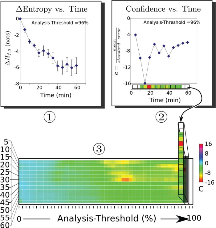
Use of $\Delta H_{f,g}$ vs time plots to prepare confidence, c, panels. Step 1: An analysis threshold is set, and $H_{f,g}$ images are analyzed to produce plots of $\Delta H_{f,g}$; the time plot for the 96% analysis threshold is shown. Step 2: The confidence as a function of time is computed according to Eq. 6 and then converted to a color bar shown parallel to the x axis of the plot. Step 3: These color bars are stacked vertically left-to-right, in increasing order, to prepare a confidence panel showing the confidence obtained at all time points for all analysis thresholds between 0% and100%. A color-to-confidence calibration bar is shown to the right of the confidence panel.

Medical imaging: Targeted tumor imaging

Previously, we reported on application of entropic quantifies $H_f$ and $I_{f,\infty }$ for detection of subtle changes in RF backscatter induced by accumulation of targeted nanoscale contrast enhancers in tumor neovasculature6, 8 or pre-cancerous tissue.7 We have used the same raw RF from these studies to prepare $H_{f,g}$ images, which were then analyzed for evidence of nanoparticle accumulation. As the materials and methods for these studies are described in previous publications,8 we provide only a brief summary of data acquisition and analysis in each case and then present a comparison of the $H_{f,g}$ and $I_{f,\infty }$ analyses.

MDA 435 tumors implanted in athymic nude mice

Human MDA 435 cancer cells were implanted in the inguinal fat pads of 15 athymic nude mice between 19 and 20 days prior to acquisition of data. Five of these animals were injected with ${\alpha }_v{\beta }_3$-targeted nanoparticles, five were injected with nontargeted nanoparticles, and five were injected with saline at a whole body dose of 1 ml/kg. In addition, 15 athymic nude mice not implanted with tumors were imaged in the same region following the same imaging protocol: five were injected with ${\alpha }_v{\beta }_3$-targeted nanoparticles, five were injected with nontargeted nanoparticles, and five were injected with saline.

RF data were acquired with a research ultrasound system (Vevo 660, Visualsonics, Toronto, Canada) at 0 through 60 min in 5-min intervals after injection. The tumor was imaged with a 35-MHz center frequency single element “wobbler” probe, and the digitized RF data corresponding to single frames were stored on a hard disk for later off-line analysis. The frames consisted of 384 lines of 2048 12-bit words acquired at a sampling rate of 200 MHz using a Gage 12400 digitizer card (connected to the analog-out and sync ports of the Vevo) in a controller PC. Each frame corresponds spatially to a region 1.5 cm wide and 0.8 cm deep. Further description of materials and methods may be found in previous publications.8 The reference trace $g(t)$ was obtained by digitizing a reflection of the imaging system's interrogating pulse from a water-agarose interface using the same acquisition parameters. As for the materials study, the long-term stability of the system electronics has been verified better than the 40 dB level. Consequently, one reference trace was acquired prior to beginning the study and used for all subsequent $H_{f,g}$ analysis.

A moving window analysis was performed on each waveform by moving a rectangular window (128 points long, 0.64 μs) in 0.08 μs steps (16 points), resulting in 121 window positions within the output data set. A smoothing spline was fit to each window. Issues surrounding signal-to-noise (SNR) ratio, SNR estimation, and robust noise suppression for these data have been discussed in a previous publication.8 The fitting routine also returned an array of first and second derivatives at the locations of any critical points in the window. The arrays were used to compute $H_{f,g}$ (or $I_{f,\infty }$). This produced an image for each time point in the experiment (i.e., 0, 5,…, 60 min).

The segment of RF within the boxcar, or moving window, is processed to produce a pixel value for an $H_{f,g}$ (or $I_{f,\infty }$) image. For each mouse used in this study, this is done using RF data acquired at 0, 5,…, 60 min post-injection to produce an image at each time point. For this study, in which the same portion of the anatomy was imaged at successive intervals, our goal was to identify and quantify the accumulation of targeted nanoparticles, which occurs preferentially at targeting sites. This suggests that segmenting the image into “targeted” and “non-targeted” regions will be required as part of the analysis.

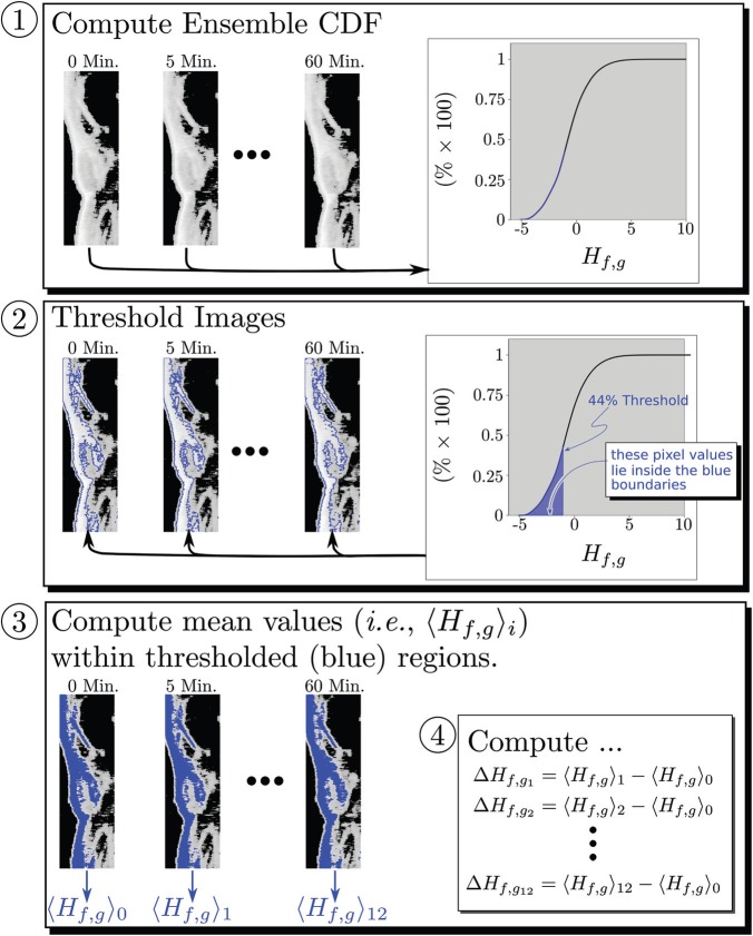
One of the chief goals of our research has been to develop objective segmentation algorithms that do not require user selection (e.g., hand drawn regions of interest). Figure 5, displays the steps of such an algorithm graphically. For each mouse used in this study, a histogram of the image pixel values appearing over the entire time course (i.e., 0, 5, 10,…, 60 min) was constructed and normalized to obtain the probability density function (PDF) of these values and then integrated to obtain the cumulative distribution function (CDF). This is shown in the top panel of the figure. Next, pixel values corresponding to “analysis-thresholds” at the lower 2%, 4%, …, 98% of the CDF were then used to segment the images at each time point into two regions corresponding to targeted and nontargeted tissue. The figure shows the segmentation for an example analysis-threshold of 44%. The blue lines, shown in the second panel of the figure, indicate the boundary between targeted (inside the blue boundaries) and non-targeted (outside the blue boundaries) regions. Subsequently, the mean value of pixels in the targeted region were computed as a function of time post-injection. This is indicated in the bottom panel of the figure, in which the mean value of $H_{f,g}$ found at each time, denoted in the figure by ${\langle H_{f,g}\rangle }_i$, i = 1,…, 12, is shown immediately below the thresholded image. Subsequently, the change in these mean values,

$$\Delta H_{f,g}={\langle H_{f,g}\rangle }_i-{\langle H_{f,g}\rangle }_0,$$ (5)

is computed ($\Delta H_{f,g_0}\hspace{0.17em}=\hspace{0.17em}0$). The analysis diagrammed in Fig. 5 was performed for all animals in all groups and the results averaged by group. We will drop the subscript i in the remaining discussion and refer only to the $\Delta H_{f,g}$.

Figure 5.

Analysis steps for $H_{f,g}$ images from a single mouse. Step 1: The cumulative distribution function (CDF) of all 12 images acquired from the animal are computed. Step 2: The CDF is used to segment the image into “targeted” (inside the blue boundaries) and “non-targeted” (outside) segments according to pixel value being above or below the threshold level (44% in this case). Step 3: the mean value, ${\langle H_{f,g}\rangle }_i$, of $H_{f,g}$ is computed for each targeted region. Step 4: These are used to calculate $\Delta H_{f,g_i}={\langle H_{f,g}\rangle }_i-{\langle H_{f,g}\rangle }_0$ for each time point in the study. This procedure is repeated for all mice in each group.

$\Delta H_{f,g}$, corresponding to a 98% analysis-threshold is plotted in Fig. 6, in panel number one. For the purposes of detection, it is actually the ratio of the mean value to the standard error that is significant. We have plotted an example of these ratios (for the MDA 435 implanted group injected with ${\alpha }_v{\beta }_3$-targeted nanoparticles) in panel two of Fig. 6. To shorten subsequent discussion of our results, we will define this ratio (confidence) as19

$$\mathbf{c}=\frac{\text{mean}}{\text{standard}\hspace{0.17em}\hspace{0.17em}\text{error}}.$$ (6)

As this panel shows, for an analysis-threshold of 98%, the mean value of $\Delta H_{f,g}$ is at all times at least four standard deviations or more from zero and peaks at 16 standard deviations from the mean $H_{f,g}$ at zero time. We have mapped each confidence value to a color scale shown along the x axis of the plot. Panel three of the figure shows the aggregate of all color maps resulting from analysis thresholds between 0% and 98%. These aggregated color maps, or confidence panels, may be used to quickly identify analysis thresholds at which accumulation of targeted nanoparticles is successfully detected by either $H_{f,g}$ or $I_{f,\infty }$ imaging and to quantify the sensitivity of each image type.

An inter-receiver comparison is shown in Fig. 7, which is a five-dimensional presentation having three dimensions within each confidence panel (i.e., post-injection time in the vertical direction, analysis-threshold in the horizontal direction, and confidence c in the out-of-plane or color direction), another dimension for animal group (the vertical direction within the array), and a fifth dimension being the masking level for the absolute value of confidence ratio c (the horizontal direction within the array). In the left column are $\Delta H_{f,g}$ confidence panels for all six groups used in our study as indicated in the figure caption. In the right-hand column are the corresponding $\Delta I_{f,\infty }$ confidence panels made using the same RF data and smoothing spline processing parameters.

In spite of the high dimensionality of the display, rapid comparison of $H_{f,g}$ or $I_{f,\infty }$ processing is possible, as well as inter-group comparison. For instance, in both columns of the top row, we observe “extensive” (meaning contiguous, wider than three columns over at least half the height of the confidence panel) regions, corresponding to confidence values greater than four in magnitude. The remaining confidence panels (for the control groups), with one exception, have much lower confidence value magnitudes in the same range of analysis-thresholds. Comparison of the confidence panels in the left column ($\Delta H_{f,g}$) shows that the top confidence panel, corresponding to the MDA 435-implanted group injected with ${\alpha }_v{\beta }_3$-targeted nanoparticles, generally exhibits confidence ratios with the greatest magnitude. There is an anomalous region of high confidence ratio for the saline group C appearing at 30 min post-injection. Because no nanoparticles were injected into this group, it might be classified as a “false-positive” for the technique. Further research, aimed at understanding and eliminating this effect, e.g., by using different reference traces $g(t)$, is underway. However, we remark that this region is contained in a range of analysis thresholds that does not overlap the range of analysis thresholds for which the confidence ratio of the targeted MDA435-implanted group (row A) is large. Consequently, it possible to define a strategy for separating the groups that eliminates false positives. Moreover, for the top row, the $\Delta H_{f,g}$ images produce confidence values that are more than twice those obtained using $\Delta I_{f,\infty }$ images. Consequently, the criteria: “$|\hspace{0.17em}\mathbf{c}\hspace{0.17em}|\hspace{0.17em}\ge \hspace{0.17em}4$,” with analysis threshold between 60% and 98% for $H_{f,g}$ analysis (44%–62% for $I_{f,\infty }$ analysis), becomes a means of distinguishing the targeted/tumor-implanted group from all others. We observe also that these criteria exhibit the presence of targeted nanoparticles accumulating within five minutes after injection. While the figure shows that we may distinguish the targeted tumor-implanted group from the control groups, the issue of single animal “diagnosis” remains open due to the small cohort of animals studied. The current study is a demonstration of feasibility and suggests the utility of conducting a larger experiment having a proper receiver operator curve analysis that would permit quantification of true positives, true negatives, false positives, and false negatives.

Transgenic K14-HPV16 mouse tumor model

The model used is the transgenic K14-HPV16 mouse that contains human papilloma virus-16 oncoproteins driven by a keratin promoter so that lesions develop in the skin, particularly in the ear. Typically the ears exhibit squamous metaplasia, a pre-cancerous condition, associated with abundant neovasculature that expresses the ${\alpha }_v{\beta }_3$ integrin. Eight transgenic mice20, 21 were treated with 1.0 mg/kg i.v. of either ${\alpha }_v{\beta }_3$-targeted nanoparticles (n = 4) or nontargeted nanoparticles (n = 4) and imaged dynamically for 1 h using a research ultrasound imager (Vevo 660 40 MHz probe) modified to store digitized RF waveforms acquired at 0, 15, 30, and 60 min. time points. Further details may be found in reference 8. All RF data were processed in the same manner as the MDA 435 data.

The results are shown in Fig. 8, which displays the three confidence panels obtained using $H_{f,g}$ images on the left and $I_{f,\infty }$ images on the right. Broad, contiguous, regions of large confidence ratio magnitude only occur in the right side of the panels, corresponding to analysis thresholds of 78% to 98%. Consequently, we have emphasized these portions by enclosing them with dotted lines while placing a semi-transparent layer over the complementary region (which has been displayed in this manner for completeness). Focusing attention on the 78% to 98% confidence thresholds, we see that $H_{f,g}$ analysis exhibits twice the sensitivity of $I_{f,\infty }$ analysis for the targeted group. Moreover, $H_{f,g}$ analysis, at these analysis thresholds, exhibits greater separation between the targeted group and the saline control group than does $I_{f,\infty }$ analysis. While separation between the targeted group and the non-targeted control is greater for $I_{f,\infty }$ analysis, the panels show that $H_{f,g}$ analysis still yields several standard deviations of separation between the two groups.

DISCUSSION AND CONCLUSIONS

In all cases, the sensitivity afforded by analysis of $H_{f,g}$ images exceeds that obtained in our best previous analyses of the same data by roughly a factor of 2. The main difference between the previous approach and the current one is employment of a reference trace. The results presented in this study employed a reference, water-path only reflection from a weak reflector, which is the natural choice in many conventional ultrasonic analyses that deconvolve the transfer function of the experimental apparatus from the raw experimental data. In our case, the rationale for application of this reference is based on the relation between entropy, $H(A)$, joint entropy, $H(A,B)$, and conditional entropy of B given A, $H(B|A)$ for discrete random variables A, and B, which is

$$H(B,A)=H(A,B)=H(A)+H(B|A).$$ (7)

If A is taken as a reference variable and we compute $H(B\prime ,A)$ where $B\prime$ is another random variable, then $H(B,A)-H(B\prime ,A)=H(B|A)-H(B\prime |A)$. Because analysis of entropy images described in the preceding text is based on differences between joint entropies, the last equation shows that they can be reinterpreted as differences between conditional entropies, i.e., heuristically at least, we are looking at the differences in information contained in backscattered RF (e.g., either B, or $B\prime$) given that the tissue was interrogated with a certain reference pulse (A).

The reference trace $g(t)$ is also a “knob” that we can “turn” to adjust the sensitivity of the image to specific attributes in the reference waveform. In our heuristic interpretation, we are examining the extent of differences between the information in the reference trace and the backscatter. In other words, we are estimating how much the information content of the interrogating ultrasonic pulse has been changed by the scattering events occurring in the tissue.

In spite of the fact that our choice of reference appears natural, it is conceivable that in other circumstances, a different choice of reference waveform might be more compelling. Thus the choice of reference is to some extent arbitrary. Our response to this fact has been to post-process the resulting $H_{f,g}$ images using all analysis thresholds and to determine if there exists a rational set of criterion for differentiating the targeted from control groups. The results of the present study, as well as previous studies,8, 15 advance one strategy for doing so. The investigation of other strategies for choice of an optimum reference given specific detection requirements is the subject of ongoing research.

APPENDIX A: CALCULATION OVERVIEW

In this subsection, we derive from Eq. 2 an expression for $H_{f,g}$ in terms of the experimentally accessible quantities $f(t)$ and $g(t)$. To do this, we claim the following assertions, which will be established in subsequent sections:

• (a)Claim i:$p^{\Delta }(j,k)=\Delta t_i=t_{i+1}-t_i$ if $\gamma (t)$ enters the $(j,k)\text{th}$ cell at time $t_i$ and leaves it at $t_{i+1}$. Otherwise, $p^{\Delta }(j,k)=0$. This is Eq. B28 in the following text. Consequently, evaluation of Eq. 3 comes down to being able to compute the limiting behavior of $\epsilon \Delta t_i\hspace{0.17em}\text{log}[\Delta t_i]$ as $\epsilon \to 0$. We will see presently that what we really need to compute is the limiting behavior of $\epsilon \Delta s_i\hspace{0.17em}\log [\Delta s_i]$.

This leads us to our second assertion:

• (b)
  Claim ii: there exists an expression for the limiting behavior of $\epsilon \Delta s_i\hspace{0.17em}\log [\Delta s_i]$ in terms of $f\prime (t)$ and $g\prime (t)$, assuming that $g\prime (t)/f\prime (t)$ is irrational. This is essentially Eq. A9 in the following text. Subsequently, we derive the expression for $H_{f,g}$ in terms of the experimentally accessible quantities $f\prime (t)$ and $g\prime (t)$. The next two subsections will justify claims i and ii. At this point, we observe from Fig. 9 that the distance traversed, $\Delta s_i$, in any member of $C_i$ is given by

  $$\Delta s_i=\Delta t_i{v}_i,$$ (A1)
  where $v_i=v(t_i)$, $i=\dots ,M$. Using Eq. A1, Eq. 3 becomes the sum

  $$\begin{array}{c}{\displaystyle \sum }_{i=1}^M\Delta t_i\hspace{0.17em}\log [\Delta t_i]={\displaystyle \sum }_1^M\Delta t_i\hspace{0.17em}\log \left[\frac{\Delta s_i}{v_i}\right]\\ =-{\displaystyle \sum }_{i=1}^M\Delta t_i\hspace{0.17em}\log \left[v_i\right]+{\displaystyle \sum }_{i=1}^M\Delta t_i\hspace{0.17em}\log \left[\Delta s_i\right].\end{array}$$ (A2)
  The first term in the sum has the limiting behavior

  $$-{\displaystyle \sum }_{i=1}^M\Delta t_i\hspace{0.17em}\text{log}\left[v_i\right]\to -{\displaystyle {\int }_0^1\mathit{dt}\hspace{0.17em}\text{log}\left[v(t)\right],}$$ (A3)
  as $\epsilon \to 0$. It remains to evaluate the sum

  $${\displaystyle \sum }_{i=1}^M\Delta t_i\hspace{0.17em}\log \left[\Delta s_i\right].$$ (A4)
  However, we do not know the coordinates of the entry (or exit) points of $\gamma (t)$ into the $i\text{th}$ cell, and thus it appears that we lack the necessary information to calculate either $\Delta t_i$ or $\Delta s_i$. Nevertheless, if we assume that the portion of the curve $\gamma (t)$ within each $\epsilon \times \epsilon$ cell is a straight line segment that starts at the point $(f(t_i),g(t_i))$ and has slope

  $${\alpha }_i\equiv g\prime (t_i)\hspace{0.17em}/\hspace{0.17em}f\prime (t_i)$$ (A5)
  so that it leaves the $\epsilon \times \epsilon$ cell near the point $(f(t_{i+1}),g(t_{i+1}))$, we may then continue the limiting process by sub-partitioning each cell further into ${\epsilon }_s\times {\epsilon }_s$ cells as shown in Fig. 10. Given this subdivision, each term in the sum, Eq. A4, must now be replaced by the sum

  $${\displaystyle \sum }_{n=1}^{M_{S_i}}\Delta t_{i,n}\log \left[\Delta s_{i,n}\right],$$ (A6)
  where the n indexes the ${\epsilon }_s\times {\epsilon }_s$ cells crossed by $\gamma (t)$ as it traverses the larger $\epsilon \times \epsilon$ cell. Thus the sum appearing in Eq. A4 is replaced by a double sum

  $${\displaystyle \sum }_{i=1}^M{\displaystyle \sum }_{n=1}^{M_{S_i}}\Delta t_{i,n}\log \left[\Delta s_{i,n}\right].$$ (A7)
  We further assume that the velocity, $v_i$, is constant over the entire $\epsilon \times \epsilon$ square as we further subdivide it. Thus the inner sum in Eq. A6 becomes

  $$\begin{array}{c}{\displaystyle \sum }_{n=1}^{M_S}\Delta t_{i,n}\hspace{0.17em}\log \left[\Delta s_{i,n}\right]={\displaystyle \sum }_{n=1}^{M_S}\frac{1}{v_i}\Delta s_{i,n}\hspace{0.17em}\log \left[\Delta s_{i,n}\right]\\ =\frac{1}{v_i}{\displaystyle \sum }_{n=1}^{M_S}\Delta s_{i,n}\hspace{0.17em}\log \left[\Delta s_{i,n}\right]\\ \equiv {\mathit{S}}_{\mathit{i}}\mathit{.}\end{array}$$ (A8)

  While it remains true that we still do not know where $\gamma (t)$ will enter each of these smaller cells, we have nevertheless made progress because if we imagine stacking all of the ${\epsilon }_s\times {\epsilon }_s$ cells crossed by $\gamma (t)$ on top of each other, as shown in Fig. 11, we will observe that, in almost every case (we will make this statement precise presently), the entry/exit points will be uniformly distributed around the perimeter of the smaller ${\epsilon }_s\times {\epsilon }_s$ cell. Given this picture, it is relatively easy to see that $\Delta s_i$ may be obtained by summing the transit lengths of $\gamma (t)$ over the smaller “stacked” ${\epsilon }_s\times {\epsilon }_s$ cell and that in the limit where these crossings become infinite (i.e., ${\epsilon }_s\to 0$), the sum may be obtained as the integral of the transit lengths, starting along the boundary of the stacked cell.

Figure 10.

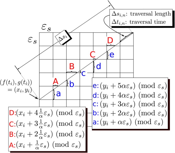
(Color online) Subdivision of an $\epsilon \times \epsilon$ cell into finer ${\epsilon }_s\times {\epsilon }_s$ cells required for evaluation of Eq. A6. We assume that ε is small enough that in the larger $\epsilon \times \epsilon$ cell $\gamma (t)$ is a straight line and $v(t)$ is constant. Legends indicate lengths of lettered segments.

Figure 11.

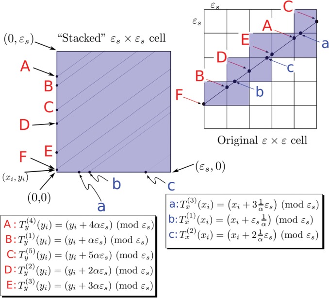
(Color online) Mapping of subgrids onto the “stacked” ${\epsilon }_s\times {\epsilon }_s$ square. The shaded ${\epsilon }_s\times {\epsilon }_s$ sub-squares of the original $\epsilon \times \epsilon$ cell are all stacked on top of each other. The corresponding points where $\gamma (t)$ crosses boundaries of the sub-squares are lettered by capital or small letters. Legends indicates their status as iterates of the mapping $T_y(y_i)$ or $T_x(x_i)$ [Eqs. C4, C6]. For irrational ${\alpha }_i=g\prime (t_i)/f\prime (t_i)$, the ergodic theorem guarantees that as the number of sub-squares is increased, the density of labeled points on vertical and horizontal sides becomes uniform.

The almost every case in the preceding text occurs when the ratio $g\prime (t)\hspace{0.17em}/\hspace{0.17em}f\prime (t)$ is irrational. The reader might anticipate this fact by considering first the case where the ratio is rational (and the lengths of the sides of the ${\epsilon }_s\times {\epsilon }_s$ cell is rational, which is the case with our conventions), then it is easy to see that a small set of entry/exit points will be used over and over again, i.e., the trajectory cell crossings will exhibit periodic behavior. It is also relatively easy to see that the number of these entry/exit points grows as the decimal expansion of the $g\prime (t)\hspace{0.17em}/\hspace{0.17em}f\prime (t)$ grows in length. Consequently, we might anticipate that for irrational $g\prime (t)\hspace{0.17em}/\hspace{0.17em}f\prime (t)$, the number of these points is infinite. The ergodic theorem tells us that this is, in fact, true and that they are also uniformly distributed around the perimeter of the ${\epsilon }_s\times {\epsilon }_s$ cell. Thus the entry point into the original (larger) $\epsilon \times \epsilon$ cell becomes irrelevant because as the ${\epsilon }_s\times {\epsilon }_s$ cells are made smaller, all entry values occur with equal probability. Actually, while application of the ergodic theorem eliminates that we know where $\gamma (t)$ enters a cell, it also introduces a cell dependent scaling factor into our expression for $\Delta s_i$. Consequently, we have traded one missing piece of information for another. However, these scaling factors group together in the course of the calculation can be eliminated from the final expression for ${\mathit{S}}_i$ [see Eq. C18]. Moreover, if $f(t)$, $g(t)$ are continuously differentiable over their range, then the set of points at which $f\prime (t)/g\prime (t)$ is rational forms a set of measure zero, which may be ignored in any integral, so that it is only the cases where $g\prime (t)\hspace{0.17em}/\hspace{0.17em}f\prime (t)$ is irrational that matter. We provide the precise details in a subsequent section, the end result is:

$$\begin{array}{c}{\mathit{S}}_{\mathit{i}}=\frac{1}{v_i}{\displaystyle \sum }_{n=1}^{M_S}\Delta s_{i,n}\hspace{0.17em}\log \left[\Delta s_{i,n}\right]\\ =-\frac{1}{2}\frac{1}{v_i}\Delta s_i\frac{\text{min}[|\hspace{0.17em}f\prime (t_i)\hspace{0.17em}|,|\hspace{0.17em}g\prime (t_i)\hspace{0.17em}|]}{\text{max}[|\hspace{0.17em}f\prime (t_i)\hspace{0.17em}|,|\hspace{0.17em}g\prime (t_i)\hspace{0.17em}|]}\\ +\frac{1}{v_i}\Delta s_i\hspace{0.17em}\log \left[\sqrt{1+{\left(\frac{\text{min}[|\hspace{0.17em}f\prime (t_i)\hspace{0.17em}|,|\hspace{0.17em}g\prime (t_i)\hspace{0.17em}|]}{\text{max}[|\hspace{0.17em}f\prime (t_i)\hspace{0.17em}|,|\hspace{0.17em}g\prime (t_i)\hspace{0.17em}|]}\right)}^2}\right]\\ +\frac{1}{v_i}\Delta s_i\hspace{0.17em}\log [{\epsilon }_s]\\ =-\frac{1}{2}\Delta t_i\frac{\text{min}[|\hspace{0.17em}f\prime (t_i)\hspace{0.17em}|,|\hspace{0.17em}g\prime (t_i)\hspace{0.17em}|]}{\text{max}[|\hspace{0.17em}f\prime (t_i)\hspace{0.17em}|,|\hspace{0.17em}g\prime (t_i)\hspace{0.17em}|]}\\ +\Delta t_i\hspace{0.17em}\log \left[\sqrt{1+{\left(\frac{\text{min}[|\hspace{0.17em}f\prime (t_i)\hspace{0.17em}|,|\hspace{0.17em}g\prime (t_i)\hspace{0.17em}|]}{\text{max}[|\hspace{0.17em}f\prime (t_i)\hspace{0.17em}|,|\hspace{0.17em}g\prime (t_i)\hspace{0.17em}|]}\right)}^2}\right]\\ +\Delta t_i\hspace{0.17em}\log [{\epsilon }_s].\end{array}$$ (A9)

Summing these ${\mathit{S}}_{\mathit{i}}$ over i, we obtain

$$\begin{array}{c}{\displaystyle \sum }_{i=1}^M\left(-\frac{1}{2}\Delta t_i\frac{\text{min}[|\hspace{0.17em}f\prime (t_i)\hspace{0.17em}|,|\hspace{0.17em}g\prime (t_i)\hspace{0.17em}|]}{\text{max}[|\hspace{0.17em}f\prime (t_i)\hspace{0.17em}|,|\hspace{0.17em}g\prime (t_i)\hspace{0.17em}|]}\right)\\ +{\displaystyle \sum }_{i=1}^M\Delta t_i\hspace{0.17em}\text{log}\left[\sqrt{1+{\left(\frac{\text{min}[|\hspace{0.17em}f\prime (t_i)\hspace{0.17em}|,|\hspace{0.17em}g\prime (t_i)\hspace{0.17em}|]}{\text{max}[|\hspace{0.17em}f\prime (t_i)\hspace{0.17em}|,|\hspace{0.17em}g\prime (t_i)\hspace{0.17em}|]}\right)}^2}\right]\\ +{\displaystyle \sum }_{i=1}^M\Delta t_i\hspace{0.17em}\text{log}[{\epsilon }_s].\end{array}$$ (A10)

The last term sums to $\log [{\epsilon }_s]$ because the time required to traverse the curve is one. The remaining terms become integrals in the limit where $\epsilon \to 0$. Collecting all terms

$$\begin{array}{c}{H}^{\Delta }(f,g)\to \\ -{\displaystyle {\int }_0^1\hspace{0.17em}\mathit{dt}\hspace{0.17em}\text{log}\left[v(t)\right]}-\frac{1}{2}{\displaystyle {\int }_0^1\hspace{0.17em}\mathit{dt}\frac{\text{min}[|\hspace{0.17em}f\prime (t)\hspace{0.17em}|,|\hspace{0.17em}g\prime (t)\hspace{0.17em}|]}{\text{max}[|\hspace{0.17em}f\prime (t)\hspace{0.17em}|,|\hspace{0.17em}g\prime (t)\hspace{0.17em}|]}}\\ +\hspace{0.17em}{\displaystyle {\int }_0^1\mathit{dt}\hspace{0.17em}\text{log}}\left[\sqrt{1+{\left(\frac{\text{min}[|\hspace{0.17em}f\prime (t_i)\hspace{0.17em}|,|\hspace{0.17em}g\prime (t_i)\hspace{0.17em}|]}{\text{max}[|\hspace{0.17em}f\prime (t_i)\hspace{0.17em}|,|\hspace{0.17em}g\prime (t_i)\hspace{0.17em}|]}\right)}^2}\right]\\ +\hspace{0.17em}\text{log}[{\epsilon }_s],\end{array}$$ (A11)

as ${\epsilon }_s\to 0$. Because the form of the singularity in this limit $\log [{\epsilon }_s]$ is independent of $f(t)$ and $g(t)$, it makes sense to define

$$\begin{array}{c}{H}_{f,g}\equiv -{\displaystyle {\int }_0^{1}dt\hspace{0.17em}\log \left[v(t)\right]}-\frac{1}{2}{\displaystyle {\int }_0^{1}dt\hspace{0.17em}\frac{\text{min}[|\hspace{0.17em}f\prime (t)\hspace{0.17em}|,|\hspace{0.17em}g\prime (t)\hspace{0.17em}|]}{\text{max}[|\hspace{0.17em}f\prime (t)\hspace{0.17em}|,|\hspace{0.17em}g\prime (t)\hspace{0.17em}|]}}\\ +{\displaystyle {\int }_0^{1}dt\hspace{0.17em}\log }\left[\sqrt{1+{\left(\frac{\text{min}[|\hspace{0.17em}f\prime (t_i)\hspace{0.17em}|,|\hspace{0.17em}g\prime (t_i)\hspace{0.17em}|]}{\text{max}[|\hspace{0.17em}f\prime (t_i)\hspace{0.17em}|,|\hspace{0.17em}g\prime (t_i)\hspace{0.17em}|]}\right)}^2}\right].\end{array}$$ (A12)

We observe that this expression is completely symmetric in $f(t)$ and $g(t)$ as expected.

Moreover, because

$$\sqrt{1+{\left(\frac{\text{min}[|\hspace{0.17em}f\prime (t)\hspace{0.17em}|,|\hspace{0.17em}g\prime (t)\hspace{0.17em}|]}{\text{max}[|\hspace{0.17em}f\prime (t)\hspace{0.17em}|,|\hspace{0.17em}g\prime (t)\hspace{0.17em}|]}\right)}^2}$$

is equal to

$$\begin{array}{c}=\sqrt{{\left(\frac{\text{max}[|\hspace{0.17em}f\prime (t)\hspace{0.17em}|,|\hspace{0.17em}g\prime (t)\hspace{0.17em}|]}{\text{max}[|\hspace{0.17em}f\prime (t)\hspace{0.17em}|,|\hspace{0.17em}g\prime (t)\hspace{0.17em}|]}\right)}^2+{\left(\frac{\text{min}[|\hspace{0.17em}f\prime (t)\hspace{0.17em}|,|\hspace{0.17em}g\prime (t)\hspace{0.17em}|]}{\text{max}[|\hspace{0.17em}f\prime (t)\hspace{0.17em}|,|\hspace{0.17em}g\prime (t)\hspace{0.17em}|]}\right)}^2}\\ =\sqrt{\frac{\text{min}{[|\hspace{0.17em}f\prime (t)\hspace{0.17em}|,|\hspace{0.17em}g\prime (t)\hspace{0.17em}|]}^2+\text{max}{[|\hspace{0.17em}f\prime (t)\hspace{0.17em}|,|\hspace{0.17em}g\prime (t)\hspace{0.17em}|]}^2}{\text{max}{[|\hspace{0.17em}f\prime (t)\hspace{0.17em}|,|\hspace{0.17em}g\prime (t)\hspace{0.17em}|]}^2}}\\ =\sqrt{\frac{f\prime {(t)}^2+g\prime {(t)}^2}{\text{max}{[|\hspace{0.17em}f\prime (t)\hspace{0.17em}|,|\hspace{0.17em}g\prime (t)\hspace{0.17em}|]}^2}}\\ =\frac{v(t)}{\sqrt{\text{max}{[|\hspace{0.17em}f\prime (t)\hspace{0.17em}|,|\hspace{0.17em}g\prime (t)\hspace{0.17em}|]}^2}},\end{array}$$ (A13)

Eq. A11 becomes

$$\begin{array}{c}{H}_{f,g}\equiv -\frac{1}{2}{\displaystyle {\int }_0^1\hspace{0.17em}dt}\hspace{0.17em}\frac{\text{min}[|\hspace{0.17em}f\prime (t)\hspace{0.17em}|,|\hspace{0.17em}g\prime (t)\hspace{0.17em}|]}{\text{max}[|\hspace{0.17em}f\prime (t)\hspace{0.17em}|,|\hspace{0.17em}g\prime (t)\hspace{0.17em}|]}\\ -{\displaystyle {\int }_0^1\hspace{0.17em}dt\hspace{0.17em}\log \hspace{0.17em}[|\hspace{0.17em}\text{max}[|\hspace{0.17em}f\prime (t)\hspace{0.17em}|,|\hspace{0.17em}g\prime (t)\hspace{0.17em}|]\hspace{0.17em}|]}\hspace{0.17em}.\end{array}$$ (A14)

Before proceeding to the claims, we point out that in this study, we consider only the case where self-intersections of $\gamma (t)$ are isolated as shown in Figs. 1, 12, and 14. Inspection of our experimental data shows that this assumption is valid in all but a negligible number of cases, which have been “masked” as described in the following text and excluded from analysis. In the case of complete overlap, where $f(t)=g(t)$, the joint entropy $H_{f,g}$ reduces effectively to $H_f$ entropy published previously.6, 7 An intermediate case, of total overlap for part of $\gamma (t)$ and isolated self-intersection on other portions can be handled by breaking up the integrals we will obtain into separate portions.

Figure 12.

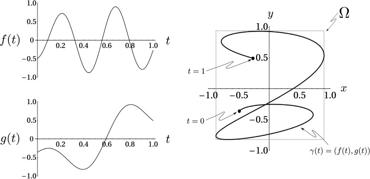
Examples of two time-domain functions, $f(t)=x$, $g(t)=y$ (left side) and the path they define, $\gamma (t)$, in the $x,y$ plane (right side). The action of the Schwartz distribution $w(x,y)$ in a two dimensional integral is to collapse it into an equivalent one dimensional integral over time.

Figure 14.

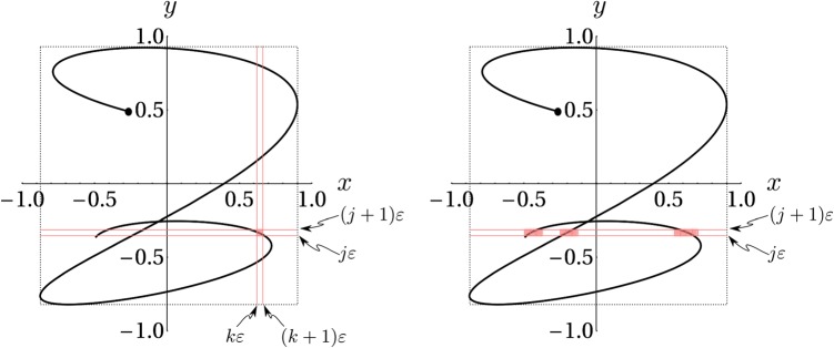
(Color online) Computation of $p(j,k)$ (left). Computation of the marginal probability $p(k)$ (right).

APPENDIX B: JUSTIFICATION OF CLAIM i

We begin by establishing the joint density $w(x,y)$ as the (Schwartz) distribution obtained from the cumulative joint density function, $W(x,y)$, for $x=f(t)$ and $y=g(t)$, While $W(x,y)$ is a conventional function of x and y, $w(x,y)$ is not, so that a course-graining operation on $w(x,y)$ using test functions must be defined. This leads to the main result of this section, Eq. B28. Although this permits computation of the course-grained joint-entropy, we must also verify consistency of this approach with that used to obtain previous entropies, e.g., $H_f$, $I_f(r)$, and $I_{f,\infty }$, which were based on the density function, $w_f(y)$ for a single function $y=f(t)$.6, 7, 8, 12, 22 This is established by showing that the marginal density functions obtained from $w(x,y)$ are just the single function densities employed previously. The same results are established for the course-grained marginal probabilities.

Calculating $\partial W(x,y)/\partial x\partial y$ using Schwartz distributions

Typically, $w(\mathit{x,y})$ is defined as the second partial derivative (with respect to x and y) of the joint cumulative density function $W(x,y)$. However, for the types of random variables, we consider (assumed to be infinitely differentiable) the joint density requires further discussion since, unlike $w_f(x)$ and $w_g(y)$,7, 12, 22 it is not a regular function (and is defined in the following text as a distribution in the sense of L. Schwartz). So we must start with the joint cumulative density function, $W(x,y)$, for $f(t)=x$, $g(t)=y$, an example of which is shown in Fig. 1. This is a regular function defined by

$$W(x,y)=\left|\{t\in ℝ:\hspace{0.17em}f(t)\le x\hspace{0.17em}\hspace{0.17em}\text{and}\hspace{0.17em}\hspace{0.17em}g(t)\le y\}\right|,$$ (B1)

where $|\hspace{0.17em}\{·\}\hspace{0.17em}|$ denotes the measure (“length”) of the set. The right side of Fig. 1 has an example calculation of $W(0.5,0.75)$ directly from Eq. B1.

On the left side of the figure, an alternative (and eventually more useful) way of looking at $W(x,y)$ is shown. The trajectory defined by

$$\gamma (t)=\left(f(t),g(t)\right),$$ (B2)

parameterized by time running from $0\to 1$, is shown. Also shown is a red box having lower left corner at the point $(\mathit{x,y})=(-1,-1)$ and its upper right corner at $(x,y)=(0.5,0.75)$. The portions of the trajectory within this rectangular region are colored red, and the entry and exit times of the red portions are labeled to show their correspondence with times in the right-hand side of the figure. The sum of these times is $W(0.5,0.75)$, so that $W(x,y)$ measures the time that the trajectory spends in the red box.

The figure also suggests that the derivative of $W(\mathit{x,y})$ will exhibit jump discontinuities for certain values of x and y as the number of segments of $\gamma (t)$ contained in the red rectangle changes discontinuously, for instance, as the height of the red rectangle is adjusted so that its top moves from below to just above the point labeled $t_0$. This result may also be anticipated by formally differentiating the integral representation of $W(x,y)$ given in Eq. B4. Consequently, careful definition of $w(x,y)$ will require the use of Schwartz distributions.

If $H(x)$ is the Heaviside function

$$H(x)=\{\begin{array}{c}0\hspace{1em}\hspace{1em}x<0,\\ 1\hspace{1em}\hspace{1em}x\ge 0,\end{array}$$ (B3)

then

$$W(x,y)={\displaystyle {\int }_0^{1}H\left(x-f(t)\right)H(y-g(t))\hspace{0.17em}dt}.$$ (B4)

We note that the joint density $w(x,y)=\left({\partial }^2/\partial x\partial y\right)W(x,y)$ appears only in expressions like

$$I={\displaystyle {\int }_{-1}^1\mathit{d}\mathit{x}}{\displaystyle {\int }_{-1}^{1}dy\hspace{0.17em}\varphi (x,y)w(x,y).}$$ (B5)

While $w(\mathrm{x,y})$ is not a regular “point” function, we recognize that it can be defined as a Schwartz distribution. Thus we assume that we may freely interchange orders of integration and that if $\varphi (x,y)\in C_c^{\infty }(\Omega )$ [recall $\Omega =(-1,1)\times (-1,-1)$], we obtain

$$\begin{array}{c}\hspace{0.17em}I={\displaystyle {\int }_{-1}^{1}dx}{\displaystyle {\int }_{-1}^{1}dy\hspace{0.17em}\varphi (x,y)w(x,y)}\\ ={\displaystyle {\int }_{-1}^{1}dx}{\displaystyle {\int }_{-1}^{1}dy\hspace{0.17em}\varphi (x,y)\frac{{\partial }^{2}W(x,y)}{\partial x\partial y}}\\ ={\displaystyle {\int }_{-1}^{1}dx}{\displaystyle {\int }_{-1}^{1}dy\frac{{\partial }^2\varphi (x,y)}{\partial x\partial y}W(x,y),}\end{array}$$ (B6)

$$\begin{array}{c}I={\displaystyle {\int }_{-1}^1\mathit{dx}}{\displaystyle {\int }_{-1}^1\mathit{dy}}\frac{{\partial }^{2}f(\mathit{x,y})}{\partial x\partial y}{\displaystyle {\int }_0^1\mathit{dtH}\hspace{0.17em}(x-f(t))}\\ \times H\hspace{0.17em}(y-g(t))\end{array}$$ (B7)

$$\begin{array}{c}={\displaystyle {\int }_0^1\mathit{d}\mathit{t}}{\displaystyle {\int }_{-1}^1\mathit{d}\mathit{x}}{\displaystyle {\int }_{-1}^1\mathit{d}\mathit{y}}\frac{{\partial }^2\varphi (x,y)}{\partial x\partial y}H(x-f(t))\\ \times H(y-g(t))\end{array}$$ (B8)

$$={\displaystyle {\int }_0^1\mathit{d}\mathit{t}}{\displaystyle {\int }_{-1}^{1}dxH(x-f(t))}$$

$$\times \left[\begin{array}{c}{\frac{\partial \varphi (x,y)}{\partial x}H(y-g(t))|}_{y=-1}^{y=1}\\ -{\displaystyle {\int }_{-1}^1\mathit{d}\mathit{y}}\frac{\partial \varphi (x,y)}{\partial x}\frac{\partial }{\partial y}H(y-g(t))\end{array}\right],$$ (B9)

$$\begin{array}{c}I=-{\displaystyle {\int }_0^1\mathit{d}\mathit{t}}{\displaystyle {\int }_{-1}^{1}dxH(x-f(t))}\\ \times {\displaystyle {\int }_{-1}^1\mathit{d}\mathit{y}}\frac{\partial \varphi (x,y)}{\partial x}\frac{\partial }{\partial y}H(y-g(t)),\end{array}$$ (B10)

where the boundary terms vanished because $\varphi (x,y)\in C_c^{\infty }(\Omega )$. Using

$${\displaystyle {\int }_{-1}^{1}dyF(x,y)\hspace{0.17em}}\frac{\partial }{\partial y}H(y-z)=F(x,z),$$ (B11)

with

$$F(x,y)=\frac{\partial \varphi (x,y)}{\partial x},$$ (B12)

Eq. B10 becomes

$$I=-{\displaystyle {\int }_0^1\mathit{dt}\hspace{0.17em}}{\displaystyle {\int }_{-1}^1\mathit{dxH}(x-f(t))}\frac{\partial \varphi (\mathrm{x,g}(t))}{\partial x}.$$ (B13)

Integrating by parts again leads to

$$I=-{\displaystyle {\int }_0^1\mathit{d}\mathit{t}}\left[\begin{array}{c}{\varphi (x,g(t))H(x-f(t))|}_{x=-1}^{x=1}\\ -{\displaystyle {\int }_{-1}^{1}dx\hspace{0.17em}}\frac{\partial }{\partial x}H(x-f(t))\varphi (x,g(t))\end{array}\right]$$ (B14)

$$={\displaystyle {\int }_0^1\mathit{d}\mathit{t}}{\displaystyle {\int }_{-1}^{1}dx\hspace{0.17em}}\frac{\partial }{\partial x}H(x-f(t))\varphi (x,g(t)),$$ (B15)

where once again the boundary terms vanish because $\varphi (x,y)\in C_c^{\infty }(\Omega )$. Using Eqs. B11, B12, Eq. B15 becomes

$$I={\displaystyle {\int }_0^1\mathit{dt}\hspace{0.17em}}\hspace{0.17em}\varphi (f(t),g(t)).$$ (B16)

Combining this result with Eq. B5, we see that, as a Schwartz distribution, $w(x,y)$ obeys the relation

$${\displaystyle {\int }_{-1}^1\mathit{d}\mathit{x}}{\displaystyle {\int }_{-1}^{1}dy\hspace{0.17em}\varphi (x,y)w(x,y)}={\displaystyle {\int }_0^{1}dt\hspace{0.17em}\varphi (f(t),g(t)).}$$ (B17)

This generalizes the expression for single (differentiable) random variable density function

$${\displaystyle {\int }_0^1\varphi (y)w_f(y)dy}={\displaystyle {\int }_0^1\varphi (f(t))dt,}$$ (B18)

which we have employed in the definition of $H_f$ as described in previous studies.6, 7, 8, 12, 22

Where $w(x,y)$ “lives” in terms of $f(t)$ and $g(t)$

Equation B16 can be visualized using the picture shown on the right-hand panel of Fig. 12. The fact that $w(x,y)$ is represented by a Schwartz distribution means that the “probability” is effectively concentrated on the curve $\gamma (t)$. Thus the current situation differs significantly from typical applications of jointly distributed random variables, which are usually distributed continuously over two-dimensional regions of the real plane.

Marginal distributions

Consistency of the current approach with previous studies requires that the marginal density functions for $w(x,y)$ obtained using Eq. B17 should be identical with the single (differential) random variable density functions of Eq. B18. To check this, we let $\varphi (x)\in C_c^{\infty }(\Omega )$ and compute

$$\begin{array}{c}I={\displaystyle {\int }_{f_{\mathit{min}}}^{f_{\mathit{max}}}\mathit{dx}}\hspace{0.17em}{\displaystyle {\int }_{g_{\mathit{min}}}^{g_{\mathit{max}}}\mathit{dy}\hspace{0.17em}\varphi (x)w(\mathrm{x,y})}\\ ={\displaystyle {\int }_0^1\mathit{dt}\hspace{0.17em}\varphi (f(t))}\\ ={\displaystyle {\int }_{f_{\mathit{min}}}^{f_{\mathit{max}}}\mathit{dx}\hspace{0.17em}\varphi (x)w_f(x).}\end{array}$$ (B19)

But also

$$\begin{array}{c}I={\displaystyle {\int }_{f_{\mathit{m}\mathit{i}\mathit{n}}}^{f_{\mathit{m}\mathit{a}\mathit{x}}}\mathit{d}\mathit{x}}\hspace{0.17em}{\displaystyle {\int }_{g_{\mathit{m}\mathit{i}\mathit{n}}}^{g_{\mathit{m}\mathit{a}\mathit{x}}}\mathit{d}\mathit{y}}\hspace{0.17em}\varphi (x)w(x,y)\\ ={\displaystyle {\int }_{f_{\mathit{m}\mathit{i}\mathit{n}}}^{f_{\mathit{m}\mathit{a}\mathit{x}}}\mathit{d}\mathit{x}}\hspace{0.17em}\varphi (x){\displaystyle {\int }_{g_{\mathit{m}\mathit{i}\mathit{n}}}^{g_{\mathit{m}\mathit{a}\mathit{x}}}\mathit{d}\mathit{y}}\hspace{0.17em}w(x,y).\end{array}$$ (B20)

Equations B19, B20 imply

$$w_f(x)={\displaystyle {\int }_{g_{\mathit{m}\mathit{i}\mathit{n}}}^{g_{\mathit{m}\mathit{a}\mathit{x}}}\mathit{d}\mathit{y}}\hspace{0.17em}\hspace{0.17em}w(x,y),$$ (B21)

and similarly

$$w_g(y)={\displaystyle {\int }_{f_{\mathit{m}\mathit{i}\mathit{n}}}^{f_{\mathit{m}\mathit{a}\mathit{x}}}\mathit{d}\mathit{x}}\hspace{0.17em}w(x,y),$$ (B22)

as required.

Choices of $\varphi (\mathrm{x,y})$ for coarse-graining

The integral equations, Eqs. B17, B18, defining $w(x,y)$ and $w_f(y)$ are all we need to compute the coarse-grained joint probabilities, $p^{\Delta }(j,k)$, and the associated coarse-grained marginal probabilities, $p^{\Delta }(j)$ and $p^{\Delta }(k)$, which we will need as intermediate quantities to obtain $H_{f,g}$.

This is accomplished by choosing an appropriate function $\varphi (\mathit{x,y})$ to use in Eq. B17 [or for the marginal probabilities: choosing an appropriate $\varphi (y)$ to use in Eq. B18]. Let $0<\epsilon \ll 1$ and let $0<s\ll 1$ be a parameter used to control the sharpness of the edges of test functions $\varphi (\mathit{x,y})$, which will be used to effect coarse-graining of the Schwartz distribution $w(x,y)$ and the density functions $w_f(x)$, and $w_g(y)$. We partition Ω into small square cells, $\epsilon \times \epsilon$ in size, over which we will compute integrals of product of test functions $\varphi (x,y)$ and $w(x,y)$, $w_f(x)$, or $w_g(y)$. The test function will be chosen so that as $s\to 0$, the coarse-graining test functions approach unit height square waves that sample $w(x,y)$, $w_f(x)$, or $w_g(y)$ over a small nonzero region. The aim is to simulate the operation of a digitizer that is sampling a one or two-dimensional function. We begin by defining an infinitely differentiable smooth function that “turns on” at $x=j\epsilon$ as x increases,

$${\varphi }_{\mathit{L,j}}(x)=\{\begin{array}{c}{e}^{-1/{\left(s\left(x-j\epsilon \right)\right)}^2},\\ 0,\end{array}\hspace{1em}\hspace{1em}\begin{array}{c}x>j\epsilon ;\\ x\le j\epsilon ,\end{array}$$ (B23)

and a corresponding smooth function that turns off at $x=(j+1)\epsilon$ as x increases

$${\varphi }_{R,j}(x)=\{\begin{array}{c}0,\\ e^{-1/{\left(s\left(x-\left(j+1\right)\epsilon \right)\right)}^2,}\end{array}\hspace{1em}\begin{array}{c}x\ge \left(j+1\right)\epsilon ,\\ x<\left(j+1\right)\epsilon .\end{array}$$ (B24)

Their product defines an infinitely differentiable step function,

$${\varphi }_j(x)={\varphi }_{\mathit{L,j}}(x){\varphi }_{\mathrm{R,j}}(x),$$ (B25)

which approaches a unit height square wave, turning on at $x=j\epsilon$ and turning off at $x=(j+1)\epsilon$, as $s\to 0$. This function may be used to “sample” a function of one variable, e.g., $f(t)=x$. Similarly ${\varphi }_k(y)$ is defined as an infinitely smooth precursor to a square wave that turns on at $y=k\epsilon$ and turns off at $y=(k+1)\epsilon$. Their product may be used to define the infinitely differentiable (in x and y) function

$${\varphi }_{j,k}(x,y)={\varphi }_j(x){\varphi }_k(y),$$ (B26)

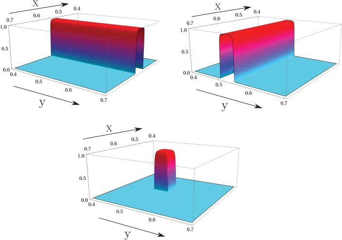
which may be used to sample functions (or Schwartz distributions) of two variables at $x=j\epsilon$, $\mathit{y}=\mathit{k\epsilon }$. Example ${\varphi }_j(x)$, ${\varphi }_k(y)$, ${\varphi }_{j,k}(x,y)$ [which are all $\in C_c^{\infty }(\Omega )$] are shown in Fig. 13.

Figure 13.

(Color online) Examples of course graining functions, ${\varphi }_j(x)$ (top left), ${\varphi }_k(y)$ (top right), and ${\varphi }_{j,k}(x,y)$ (bottom).

We will also allow the two indices, k associated with the $f(t)=x$ variable and j associated with the $g(t)=y$ variable to run from $-\infty$ to ∞.

Course-grained probabilities $p^{\Delta }(x,y)$, $p^{\Delta }(x)$, and $p^{\Delta }(y)\hspace{0.17em}\mathbf{from}$$w(x,y)$, $w_f(x)$, and $w_g(y)$

Now we have all we need to coarse-grain the densities $w(x,y)$, $w_f(x)$ and $w_g(y)$. Suppose that $\gamma (t)$ passes only once through the $j,k\text{th}$ cell, which we will denote by $C_{j,k}$. To coarse-grain $w(x,y)$ over $C_{j,k}$, we compute,

$$\begin{array}{c}{p}^{\Delta }(j,k)=\underset{s\to \infty }{\lim }{\displaystyle {\int }_{f_{\mathit{m}\mathit{i}\mathit{n}}}^{f_{\mathit{m}\mathit{a}\mathit{x}}}\mathit{d}\mathit{x}}{\displaystyle {\int }_{g_{\mathit{m}\mathit{i}\mathit{n}}}^{g_{\mathit{m}\mathit{a}\mathit{x}}}\mathit{d}\mathit{y}}\hspace{0.17em}w(x,y){\varphi }_{j,k}(x,y)\\ =\underset{s\to \infty }{\lim }{\displaystyle {\int }_0^1\mathit{d}\mathit{t}}\hspace{0.17em}{\varphi }_{j,k}(f(t),g(t))\\ =\underset{s\to \infty }{\lim }{\displaystyle {\int }_{t_i}^{t_f}\mathit{d}\mathit{t}}\hspace{0.17em}{\varphi }_{j,k}(f(t),g(t))\\ =\underset{s\to \infty }{\lim }{\displaystyle {\int }_{t_i}^{t_f}\mathit{d}\mathit{t}}=t_f-t_i,\end{array}$$ (B27)

where ${\varphi }_{j,k}(x,y)$ is defined by Eq. B26. For cells that do not intersect $\gamma (t)$, we define $p^{\Delta }(j,k)=0$ for completeness. Defining $s(t_i)$ to be the length along $\gamma (t)$ between $t=0$ and $t=t_i$, Eq. B27 may be rewritten as

$$p^{\Delta }(j,k)=t_f-t_i=\Delta t=\frac{s(t_f)-s(t_i)}{v(t_i)},$$ (B28)

where $v(t_i)=\sqrt{f\prime {(t_i)}^2+g\prime {(t_i)}^2}$ is the velocity along the curve at time $t_i$. If more than one passage through occurs $C_{j,k}$, then all traversal times $t_i$ such that $(f(t_i),g(t_i))\in \partial \hspace{0.17em}{C}_{j,k}$ must be added, and we obtain

$$p^{\Delta }(\mathit{j,k})={\displaystyle \sum }_{\{t_i\in \partial \hspace{0.17em}{C}_{\mathrm{i,j}}\}}\frac{s(t_f)-s(t_i)}{v(t_i)}.$$ (B29)

Discrete marginal probabilities: From the standard definition

The discrete marginal probabilities are defined by

$$p^{\Delta }(k)={\displaystyle \sum }_j{p}^{\Delta }(j,k).$$ (B30)

For the course-grained marginal probabilities, we also set $p^{\Delta }(k)=0$ if $\gamma (t)$ does not intersect any cell with index j ($C_{j,k}\cap \gamma (t)=0∕,\forall k$). Similarly we define,

$$p^{\Delta }(j)={\displaystyle \sum }_k{p}^{\Delta }(j,k).$$ (B31)

Discrete marginal probabilities: From Eqs. B21, B22, and B25

Alternatively, we may start with Eq. B21 and define

$$p^{\Delta }(j)={\displaystyle {\int }_{f_{\mathit{m}\mathit{i}\mathit{n}}}^{f_{\mathit{m}\mathit{a}\mathit{x}}}dx\hspace{0.17em}\hspace{0.17em}w(x,y){\varphi }_j(x),}$$ (B32)

where ${\varphi }_j(x)$ is given by Eq. B25. Similarly, using Eq. B22,

$$p^{\Delta }(k)={\displaystyle {\int }_{g_{\mathit{m}\mathit{i}\mathit{n}}}^{g_{\mathit{m}\mathit{a}\mathit{x}}}dy\hspace{0.17em}\hspace{0.17em}w(x,y){\varphi }_k(y),}$$ (B33)

where ${\varphi }_k(y)$ is also given by Eq. B25 and $p^{\Delta }(j)$, $p^{\Delta }(j)$ are zero in the same cases described after Eqs. B30, B31. Focusing on Eq. B29, we see from Fig. 14, that the integral will reduce, in the limit where $s\to \infty$, to the sum of times spent in the cells lying between $j\epsilon$ and $(j+1)\epsilon$, so that we again obtain

$$p^{\Delta }(j)={\displaystyle \sum }_k{p}^{\Delta }(\mathit{j,k})$$ (B34)

and

$$p^{\Delta }(k)={\displaystyle \sum }_j{p}^{\Delta }(j,k).$$ (B35)

We note based on previous work that as $\epsilon \to 0$ these are asymptotic to

$$p^{\Delta }(j)\sim \epsilon w_f(-1+j\epsilon )=\epsilon w_f(x)$$ (B36)

and

$$p^{\Delta }(k)\sim \epsilon w_g(-1+\mathrm{k\epsilon })=\epsilon w_g(y).$$ (B37)

These are just the coarse-grained versions of Eqs. B21, B22 and demonstrate the consistency of computing marginals and then coarse-graining with coarse-graining and then computing marginals.

APPENDIX C: JUSTIFICATION OF CLAIM ii

While Eq. B28 gives the probabilities needed to compute joint entropies in terms of time, $\Delta t_i$, we must express it in terms of experimentally accessible quantities, which means quantities derived from the backscattered RF, $f(t)$, and the reference signal $g(t)$. The first step in this process is Eq. A1, which relates $\Delta t_i$, to $\Delta s_i$ using the velocity in the cell $v_i=\sqrt{f\prime {(t)}^2+g\prime {(t)}^2}$, However, as discussed in the preceding text, we are still faced by an apparently unsolvable problem because we do not know where $\gamma (t)$ enters the $\epsilon \times \epsilon$ cell. Moreover, we also must eliminate the coarse-graining parameter, ε from the final expressions for joint entropy, which is accomplished by taking $\epsilon \to 0$. In this section, we provide the details of our approach beginning with the “stacking” process used above which may be made rigorous using the ergodic theorem23 as we now describe. Thus we suppose that we are given a straight line segment, ℓ, of slope $\alpha =g\prime (t_i)/f\prime (t_i)$, and length $\Delta s_i$, contained in a cell of dimensions $\epsilon \times \epsilon$, such as that shown in Fig. 10. We wish to subdivide the cell into ${\epsilon }_s\times {\epsilon }_s$ sub-cells as also shown in the figure, and compute the limiting form of

$${\mathit{S}}_{\mathit{i}}\equiv {\displaystyle \sum }_{n=1}^{M_S}\Delta s_{i,n}\hspace{0.17em}\log \left[\Delta s_{i,n}\right],$$ (C1)

where

$$\Delta s_i={\displaystyle \sum }_{n=1}^{M_S}\Delta s_{i,n},$$ (C2)

and the index n keeps track of the ${\epsilon }_s\times {\epsilon }_s$ cells crossed as $\gamma (t)$ traverses the larger $\epsilon \times \epsilon$ cell. We begin, as shown in Fig. 11, by imagining that we translate all the subsegments of ℓ, to the ${\epsilon }_s\times {\epsilon }_s$ square, as shown in the left hand side of the figure (this is equivalent to the stacking procedure described in the preceding text). The y coordinates of those line segments that start out on the y axis are shown the figure. These are given by

$$T_y^{(r)}(y_i)=y_i+r\alpha {\epsilon }_s\hspace{0.17em}\text{mod}\hspace{0.17em}{\epsilon }_s,$$ (C3)

where $T_y^{(r)}(y_i)$ is the $r\text{th}$ iteration of the mapping

$$T_y(y)=y+\alpha \hspace{0.17em}\text{mod}\hspace{0.17em}{\epsilon }_s.$$ (C4)

Similarly the x coordinates of those line segments that start out on the x axis are given by

$$T_x^{(r)}(x_i)=x_i+r\frac{1}{\alpha }{\epsilon }_s\hspace{0.17em}\text{mod}\hspace{0.17em}{\epsilon }_s,$$ (C5)

where $T_x^{(r)}(x_i)$ is the $r\text{th}$ iteration of the mapping

$$T_x(x)=x+\frac{1}{\alpha }\hspace{0.17em}\text{mod}\hspace{0.17em}{\epsilon }_s.$$ (C6)

Thus the physical “stacking” procedure is implemented mathematically by iterating the maps $T_x(x)$ and $T_y(y)$. Because $g\prime (t_i)/f\prime (t_i)$ is irrational, we know that both of these mappings are ergodic.23 Hence we have the following relations between sums and integrals involving continuous functions $\varphi (x)$, $\psi (y)$ and iterates of $T_x(x)$ and $T_y(y)$,

$${\displaystyle \sum }_{r=0}^{M_{s_x}-1}\varphi \left(T_x^{(r)}(x_i)\right)\to M_{s_x}{\displaystyle {\int }_0^1\mathit{dx}\hspace{0.17em}\varphi (x),}$$ (C7)

as $\hspace{0.17em}\hspace{0.17em}{M}_{s_x}\to \infty$ and,

$${\displaystyle \sum }_{r=0}^{M_{s_y}-1}\psi \left(T_y^{(r)}(y_i)\right)\to M_{s_y}{\displaystyle {\int }_0^{1}dy\hspace{0.17em}\psi (y),}$$ (C8)

as $\hspace{0.17em}\hspace{0.17em}{M}_{s_y}\to \infty$. While it is possible to use Eqs. C7, C8 to obtain Eq. A9, we will not do so. Instead, it is simpler to refer back to Fig. 11 and observe that $M_{s_x}$ is the number of times that the line segment $y=\alpha x$ crosses the vertical lines $x=m{\epsilon }_s$, where m is a non-negative integer, and $M_{s_y}$ is the number of times that the line segment $y=\alpha x$ crosses the horizontal lines $x=q{\epsilon }_s$, where q is a non-negative integer. Furthermore, we observe that the ergodic theorem tells us, via Eqs. C7, C8, that as $s\to 0$, the crossing points become uniformly distributed along the edges of the ${\epsilon }_s\times {\epsilon }_s$ square in Fig. 11. This means that the random variable y shown in Fig. 15 is uniformly distributed. Thus the variable θ, which is a linear function of y, is also uniformly distributed over its range (the interval $[0,1]$). We will use this implication of the ergodic theorem to obtain Eq. A9.

Figure 15.

The black circle is a point where $\gamma (t)$ crosses the vertical line in the ${\epsilon }_s\times {\epsilon }_s$ sub-grid shown in Fig. (11). Because α is irrational, the values of y are uniformly distributed along the vertical side of the ${\epsilon }_s\times {\epsilon }_s$ square by the ergodic theorem. This also implies that the variable θ is uniformly distributed over its range, the interval $[0,1]$, because it is a linear function of y, as shown in the figure.

Relation between $M_{s_x}$ and $M_{s_y}$

Let $s_h$ be the horizontal distance traversed and $s_v=\left|\alpha \right|s_h$ be the vertical distance traversed (so $\Delta s_i=\sqrt{1+{\alpha }^2}{s}_h$). Then

$$M_{s_x}\in \left\{\lfloor s_h/{\epsilon }_s\rfloor ,\lceil s_h/{\epsilon }_s\rceil \right\},$$ (C9)

where $\lfloor z\rfloor$ is the largest integer $\le z$, and $\lceil z\rceil$ is the smallest integer $\ge z$. Similarly

$$M_{s_y}\in \left\{\lfloor s_v/{\epsilon }_s\rfloor ,\lceil s_v/{\epsilon }_s\rceil \right\}.$$ (C10)

As $s_v=\left|\alpha \right|s_h$, we get $M_{s_y}\to \left|\alpha \right|M_{s_x}$ as ${\epsilon }_s\to 0$.

Calculation of $\Delta s_i$

We have

$$\Delta s_i=s_h\sqrt{1+{\alpha }^2}=s_v\sqrt{1+\frac{1}{{\alpha }^2}}$$ (C11)

and

$$s_h={\epsilon }_s{M}_{s_x}$$ (C12)

with an error of at most ${\epsilon }_s$ by Eq. C9. Therefore

$$\Delta s_i\approx M_{s_x}{\epsilon }_s\sqrt{1+{\alpha }^2}=M_{s_x}\epsilon \prime ,$$ (C13)

where we have defined the symbol $\epsilon \prime ={\epsilon }_s\sqrt{1+{\alpha }^2}$ to simplify calculations in the following text.

Calculation of ${\mathit{S}}_{\mathit{i}}$

We are now ready to calculate

$${\mathit{S}}_{\mathit{i}}\equiv {\displaystyle \sum }_{n=1}^{M_S}\Delta s_{i,n}\hspace{0.17em}\log \left[\Delta s_{i,n}\right].$$

We break the calculation into two cases: $\left|\alpha \right|<1$ and $\left|\alpha \right|>1$.

Case $\left|\alpha \right|<1$: We note that $M_S=M_{s_x}+M_{s_y}$ is the number of times that the trajectory, $\gamma (t)$, crosses either a vertical or a horizontal line of the ${\epsilon }_s\times {\epsilon }_s$ sub-grid. (Because α is irrational, there is at most one occasion where it crosses both simultaneously; we can ignore this event as ${\epsilon }_s\to 0$.)

If there are two successive vertical crossings, then

$$\Delta s_{i,n}\hspace{0.17em}\log \left[\Delta s_{i,n}\right]={\epsilon }_s\sqrt{1+{\alpha }^2}\hspace{0.17em}\log \left[{\epsilon }_s\sqrt{1+{\alpha }^2}\right].$$ (C14)

As $\left|\alpha \right|<1$, if this does not happen, then there is exactly one horizontal crossing in between vertical crossings at n and $n+2$, and

$$\begin{array}{c}\Delta s_{i,n}\hspace{0.17em}\log \left[\Delta s_{i,n}\right]+\\ \Delta s_{i,n+1}\hspace{0.17em}\log \left[\Delta s_{i,n+1}\right]\\ =\theta {\epsilon }_s\sqrt{1+{\alpha }^2}\hspace{0.17em}\log \left[\theta {\epsilon }_s\sqrt{1+{\alpha }^2}\right]\\ +(1-\theta ){\epsilon }_s\sqrt{1+{\alpha }^2}\hspace{0.17em}\log \left[(1-\theta ){\epsilon }_s\sqrt{1+{\alpha }^2}\right]\end{array}$$ (C15)

for some $0<\theta <1$. By the ergodic theorem, θ will tend to a uniformly distributed random variable on $[0,1]$ as shown in Fig. 15. So letting $\epsilon \prime ={\epsilon }_s\sqrt{1+{\alpha }^2}$, the contribution from Eq. C15 is, on average,

$${\displaystyle {\int }_0^1\mathrm{d\theta }\left[\theta \epsilon \prime \hspace{0.17em}\text{log}\left[\theta \epsilon \prime \right]+(1-\theta )\epsilon \prime \hspace{0.17em}\text{log}\left[(1-\theta )\epsilon \prime \right]\right],}$$ (C16)

or

$$\epsilon \prime \hspace{0.17em}\log \hspace{0.17em}\epsilon \prime -\frac{\epsilon \prime }{2}.$$ (C17)

Of the $M_{s_x}$ vertical crossings, $M_{s_y}=\left|\alpha \right|M_{s_x}$ of them will have a horizontal crossing “sandwiched” in between and contribute the quantity shown in Eq. C17 on average; the remainder will contribute $\epsilon \prime \text{log}[\epsilon \prime ]$. Thus we obtain

$$\begin{array}{c}{\mathit{S}}_{\mathit{i}}=\left|\alpha \right|M_{s_x}\left[\epsilon \prime \hspace{0.17em}\log \hspace{0.17em}\epsilon \prime -\frac{\epsilon \prime }{2}\right]+(1-\left|\alpha \right|)M_{s_x}\left[\epsilon \prime \hspace{0.17em}\log \hspace{0.17em}\epsilon \prime \right]\\ =M_{s_x}\epsilon \prime \left\{\left|\alpha \right|\left[\log \hspace{0.17em}\epsilon \prime -\frac{1}{2}\right]+(1-|\left|\alpha \right|)\hspace{0.17em}\log \hspace{0.17em}\epsilon \prime \right\}\\ =\Delta s_i\left\{-\frac{\left|\alpha \right|}{2}+\log \hspace{0.17em}\epsilon \prime \right\}\\ =\Delta s_i\left\{-\frac{\left|\alpha \right|}{2}+\log \sqrt{1+{\alpha }^2}+\log \hspace{0.17em}{\epsilon }_s\right\}.\end{array}$$ (C18)

Case $\left|\alpha \right|>1$: If $\left|\alpha \right|>1$, we repeat the calculation with x and y “switched.” The calculation proceeds exactly as before although α must be replaced by $1/\alpha$.

Calculation summary: These results may be concisely written as

$${\mathit{S}}_{\mathit{i}}=\Delta s_i\{\begin{array}{c}\left[-\frac{1}{2}\left|\alpha \right|+\log \left[\sqrt{1+{\alpha }^2}\right]\right]+\log \left[{\epsilon }_s\right]\hspace{1em}\left|\alpha \right|\le 1,\\ \left(-\frac{1}{2}\frac{1}{\left|\alpha \right|}+\log \left[\sqrt{1+\frac{1}{{\alpha }^2}}\right]\right)+\log \left[{\epsilon }_s\right]\hspace{1em}\left|\alpha \right|\ge 1\end{array}$$ (C19)

or, recalling that $\alpha =g\prime (t)/f\prime (t)$,

$$\begin{array}{c}{\mathit{S}}_{\mathit{i}}=-\frac{1}{2}\Delta s_i\frac{\text{min}[|f\prime (t_k)|,|g\prime (t_k)|]}{\text{max}[|f\prime (t_k)|,|g\prime (t_k)|]}\\ +\hspace{0.17em}\Delta s_i\text{log}\left[\sqrt{1+{\left(\frac{\text{min}[|f\prime (t_k)|,|g\prime (t_k)|]}{\text{max}[|f\prime (t_k)|,|g\prime (t_k)|]}\right)}^2}\right]\\ +\hspace{0.17em}\Delta s_i\text{log}[{\epsilon }_s],\end{array}$$ (C20)

which is Eq. A9. This completes the derivation of $H_{f,g}$.

References

- Hughes M., “Analysis of ultrasonic waveforms using Shannon entropy,” Proc.-IEEE Ultrason. Symp. 2, 1205–1209 (1992). 10.1109/ULTSYM.1992.275884 [DOI] [Google Scholar]
- Hughes M., “Analysis of digitized waveforms using Shannon entropy,” J. Acoust. Soc. Am. 93, 892–906 (1993). 10.1121/1.405451 [DOI] [Google Scholar]
- Hughes M., “NDE imaging of flaws using rapid computation of Shannon entropy,” Proc.-IEEE Ultrason. Symp. 2, 697–700 (1993). [Google Scholar]
- Hughes M., “Analysis of digitized waveforms using Shannon entropy. II. High-speed algorithms based on Green's functions,” J. Acoust. Soc. Am. 95, 2582–2588 (1994). 10.1121/1.409828 [DOI] [Google Scholar]
- Hughes M. S., Marsh J. N., Hall C. S., Savy D., Scott M. J., Allen J. S., Lacy E. K., Carradine C., Lanza G. M., and Wickline S. A., “Characterization of digital waveforms using thermodynamic analogs: Applications to detection of materials defects,” IEEE Trans. Ultrason. Ferroelectr. Freq. Control 52, 1555 – 1564 (2005). 10.1109/TUFFC.2005.1516028 [DOI] [PubMed] [Google Scholar]
- Hughes M., Marsh J., Woodson A., Lacey E., Carradine C., Lanza G. M., and Wickline S. A., “Characterization of digital waveforms using thermodynamic analogs: Detection of contrast targeted tissue in MDA 435 tumors implanted in athymic nude mice,” Proc.-IEEE Ultrason. Symp. 1, 373–376 (2005). [DOI] [PubMed] [Google Scholar]
- Hughes M. S., McCarthy J. E., Marsh J. N., Arbeit J. M., Neumann R. G., Fuhrhop R. W., Wallace K. D., Znidersic D. R., Maurizi B. N., Baldwin S. L., Lanza G. M., and Wickline S. A., “Properties of an entropy-based signal receiver with an application to ultrasonic molecular imaging,” J. Acoust. Soc. Am. 121, 3542–3557 (2007). 10.1121/1.2722050 [DOI] [PubMed] [Google Scholar]
- Hughes M., Marsh G. M., Lanza, S. A. Wickline, J. McCarthy, B. Wickerhauser, V. annd Maurizi, and, W. K., “Improved signal processing to detect cancer by ultrasonic molecular imaging of targeted nanoparticles,” J. Acoust. Soc. Am. 129, 3756–3767 (2011). 10.1121/1.3578459 [DOI] [PMC free article] [PubMed] [Google Scholar]
- Marsh J. N., McCarthy J. E., Wickerhauser M., Arbeit J. M., Fuhrhop R. W., Wallace K. D., Lanza G. M., Wickline S. A., and Hughes M. S., “Application of real-time calculation of a limiting form of the Renyi entropy for molecular imaging of tumors,” IEEE Trans. Ultrason. Ferroelectr. Freq. Control 57, 1890–1895 (2010). 10.1109/TUFFC.2010.1630 [DOI] [PMC free article] [PubMed] [Google Scholar]
- Marsh J. N., Wallace K. D., Lanza G. M., Wickline S. A., Hughes J. E., and McCarthy M. S., “Application of a limiting form of the Renyi entropy for molecular imaging of tumors using a clinically relevant protocol,” Proc.-IEEE Ultrason. Symp. 1, 53–56 (2010). [Google Scholar]
- Wallace K. D., Marsh J., Baldwin S. L., Connolly A. M., Richard K., Lanza G. M., Wickline S. A., and Hughes M. S., “Sensitive ultrasonic delineation of steroid treatment in living dystrophic mice with energy-based and entropy-based radio frequency signal processing,” IEEE Trans. Ultrason. Ferroelectr. Freq. Control 54, 2291–2299 (2007). 10.1109/TUFFC.2007.533 [DOI] [PubMed] [Google Scholar]
- Hughes M., Marsh J., Wallace K., Donahue T., Connolly A., Lanza G. M., and Wickline S. A., “Sensitive ultrasonic detection of dystrophic skeletal muscle in patients with Duchenne's muscular dystrophy using an entropy-based signal receiver,” Ultrasound Med. Biol. 33, 1236–1243 (2007). 10.1016/j.ultrasmedbio.2007.02.007 [DOI] [PMC free article] [PubMed] [Google Scholar]
- Hughes M., Marsh J., Agyem K., McCarthy J., Maurizi B., Wickerhauser M., Lanza W. K. D. G., and Wickline S., “Use of smoothing splines for analysis of backscattered ultrasonic waveforms: Application to monitoring of steroid treatment of dystrophic mice,” IEEE Trans. Ultrason. Ferroelectr. Freq. Control 58, 2361–2369 (2011). 10.1109/TUFFC.2011.2093 [DOI] [PMC free article] [PubMed] [Google Scholar]
- Seip R., Ebbini E., and O'Donnell M., “Non-invasive detection of thermal effects due to highly focused ultrasonic fields,” Proc.-IEEE Ultrason. Symp. 2, 1229–1232 (1993). [Google Scholar]
- Hughes M. S., McCarthy J. E., Wickerhauser M., Marsh J. N., Arbeit J. M., Fuhrhop R. W., Wallace K. D., Thomas T., Smith J., Agyem K., Lanza G. M., and Wickline S. A., “Real-time calculation of a limiting form of the Renyi entropy applied to detection of subtle changes in scattering architecture,” J. Acoust. Soc. Am. 126, 2350–2358 (2009). 10.1121/1.3224714 [DOI] [PMC free article] [PubMed] [Google Scholar]
- Schwartz L., Mathematics for the Physical Sciences (Dover, New York, 2008), pp. 1–368. [Google Scholar]
- Hughes M., “A comparison of Shannon entropy versus signal energy for acoustic detection of artificially induced defects in Plexiglas,” J. Acoust. Soc. Am. 91, 2272–2275 (1992). 10.1121/1.403662 [DOI] [Google Scholar]
- Reinsch C. H., “Smoothing by spline functions,” Num. Math. 10, 177–183 (1967). 10.1007/BF02162161 [DOI] [Google Scholar]
- Sackett D. L., “Why randomized controlled trials fail but needn't. II. Failure to employ physiological statistics, or the only formula a clinician-trialist is ever likely to need (or understand!),” Can. Med. Assoc. J. 165, 1226–1237 (2001). [PMC free article] [PubMed] [Google Scholar]
- Arbeit J. M., Riley R. R., Huey B., Porter C., Kelloff G., Lubet R., Ward J. M., and Pinkel D., “DFMO chemoprevention of epidermal carcinogenesis in k14-hpv16 transgenic mice,” Cancer Res. 59, 3610–3620 (1999). [PubMed] [Google Scholar]
- Arbeit J. M., Mnger K., Howley P. M., and Hanahan D., “Progressive squamous epithelial neoplasia in k14-human papillomavirus type 16 transgenic mice,” J. Virol. 68, 4358–4368 (1994). [DOI] [PMC free article] [PubMed] [Google Scholar]
- Hughes M. S., McCarthy J. E., Marsh J. N., Arbeit J. M., Neumann R. G., Fuhrhop R. W., Wallace K. D., Thomas T., Smith J., Agyem K., Znidersic D. R., Maurizi B. N., Baldwin S. L., Lanza G. M., and Wickline S. A., “Application of Renyi entropy for ultrasonic molecular imaging,” J. Acoust. Soc. Am. 125, 3141–3145 (2009). 10.1121/1.3097489 [DOI] [PMC free article] [PubMed] [Google Scholar]
- Katok A. and Hasselblatt B., Introduction to the Modern Theory of Dynamical Systems (Cambridge University Press, Cambridge, UK, 1995), pp. 1–804. [Google Scholar]