Single breath xenon polarization transfer contrast (SB-XTC): implementation and initial results in healthy humans

Abstract

Purpose

To implement and characterize a single-breath xenon transfer contrast (SB-XTC) method to assess the fractional diffusive gas transport F in the lung: to study the dependence of F and its uniformity as a function of lung volume; to estimate local alveolar surface area per unit gas volume S_A/V_Gas from multiple diffusion time measurements of F; to evaluate the reproducibility of the measurements and the necessity of B₁ correction in cases of centric and sequential encoding.

Materials and Methods

In SB-XTC three or four gradient echo images separated by inversion/saturation pulses were collected during a breath-hold in eight healthy volunteers, allowing the mapping of F (thus S_A/V_Gas) and correction for other contributions such as T₁ relaxation, RF depletion and B₁ inhomogeneity from inherently registered data.

Results

Regional values of F and its distribution were obtained; both the mean value and heterogeneity of F increased with the decrease of lung volume. Higher values of F in the bases of the lungs in supine position were observed at lower volumes in all volunteers. Local S_A/V_Gas (with a mean ± standard deviation of $\overline{S_A/V_{\mathit{Gas}}}=89\pm 30{cm}^{-1}$) was estimated in vivo near functional residual capacity. Calibration of SB-XTC on phantoms highlighted the necessity for B₁ corrections when k-space is traversed sequentially; with centric ordering B₁ distribution correction is dispensable.

Conclusion

SB-XTC technique is implemented and validated for in vivo measurements of local S_A/V_Gas.

Introduction

Proton magnetic resonance imaging (MRI) has severe limitations in the lung due to its low tissue density and short transverse relaxation time $\left(T_2^{\ast }\right)$ owing to the extremely large area of gas-tissue interfaces present in the lungs (~ 100m²). Introduction of hyperpolarized gas MRI (1–4) offers new possibilities for pulmonary imaging. ¹²⁹ Xe is lipophilic, sensitive to its surroundings due to its sizable electronic cloud, and shows an NMR spectrum that undergoes a large range of frequency shifts (~ 200 ppm) (5) when placed in different environments, thus facilitating the separate studies of pulmonary air-sacs, septa and blood (6–8). In one such study the Chemical Shift Saturation Recovery (CSSR) technique was developed (9), where the ¹²⁹ Xe magnetization in the dissolved phase was initially destroyed by a selective RF pulse. Then during a diffusion time t_diff the ¹²⁹ Xe magnetization in the dissolved phase was replenished by diffusion of polarized xenon from the alveolar gas spaces into septal tissue and blood. For porous materials in which xenon is soluble, at short diffusion times the fractional diffusive gas transport F(t), defined as the ratio of the ¹²⁹ Xe magnetization in the dissolved phase at time t relative to that in the gas phase at t=0, is proportional to the surface area available for diffusion per unit gas volume (S_A/V_Gas)(8–10). However, since only ~2% of gaseous xenon dissolves into the lung parenchyma, direct regional S_A/V_Gas measurements using techniques like Dixon method (11–13) are very challenging and suffer from low SNR.

Ruppert et al. (14,15) developed a magnetization transfer technique, Xenon polarization Transfer Contrast (XTC) that estimates a fractional depolarization F_XTC from the measurement of the hyperpolarized gas depolarization in the lungs. In contrast to the CSSR and Dixon techniques, this is an indirect measurement of diffusive gas transport to the tissue and blood. F_XTC is fundamentally different from F_CSSR except for a special case where XTC RF pulses are 90° pulses (10,16). Ruppert et al. demonstrated the feasibility of XTC in anesthetized animals during a two-breath protocol; an extension of XTC to human subjects would require either an application of image registration methods or a development of a single-breath technique to avoid these issues altogether. Previously, there were brief reports on the development of an in vivo application of a Single-Breath XTC (SB-XTC) method (8,10,17). Very recently Dregely et al. (18) reported on another implementation of single-breath multiple exchange time XTC measurements and initial results in vivo. In this paper we report the mean F, the variance in F due to physiological heterogeneity σ_Physiol and the dependence on lung volume of these two parameters in eight healthy volunteers. We also calculate the local S_A/V_Gas map from the measurements of F performed at three diffusion times. Further, we present the details of technical implementation, calibration and reproducibility evaluation of SB-XTC measurements. And finally, we show that the k-space trajectory influences the need to correct the data for B₁ inhomogeneity.

Methods

Human Subjects

All human subject experiments were conducted in compliance with IRB and FDA IND approved protocols (for details see (19)). Informed consent was obtained from all volunteers as a prerequisite to the participation in the study. Pulmonary functional tests (PFT) were obtained on all subjects (Table 1). The gas volumes inhaled by each subject to achieve a particular lung volume were calculated based on either the measured values of residual volume (RV) and total lung capacity (TLC) or, if the MRI experiments occurred before the PFT’s were obtained, on the predicted values.

Table 1.

Subject data

Subject	sex	age	Measured
			RV, L	TLC, L	DLCO	FEV1
HS1	male	55	1.85	7.02	38.38	3.93
HS2	male	31	1.94	7.54	34.72	4.86
HS3	male	31	1.33	6.2	26.79	4.41
HS4**	female	25	1.25	4.44	20.74	2.65
HS5	female	35	1.11	4.96	21.24	3.09
HS6*	male	28	2.02	9.78	-	6.19
HS7*	male	28	1.45	8.88	-	5.82
HS8***	male	26	1.42	7.57	39.65	4.96

^*These subjects are the competitive world-class deep divers who are able to perform GE and reach lung volumes below RV. Both of them for experiments reached these volumes (RV_GE). For HS8, RV_GE=1.71 L, and for HS9, RV_GE=1.14 L.

^**This subject participated in experiments at 3T.

^***Optimization of the number of inversion pulses was performed with this subject

A total of eight healthy subjects participated in the study. Two of them were world-class deep divers, trained to perform glossopharyngeal exsufflation (GE) - a maneuver used to extract air from the lungs. Performed repeatedly, this maneuver can lower lung volume (VL) by several hundred ml below (RV) (20,21). These two subjects provided a unique opportunity to study ventilation and gas exchange at extremely low VL otherwise unattainable for in vivo studies in intact lungs (22). All subjects followed the same breathing protocol to standardize the ventilation: while inside the magnet, they were instructed to inhale to TLC and exhale to RV twice, then inhale the gas mixture and hold their breath. Both divers performed GE to reach sub-RV after their second exhalation to RV, and then inhaled the gas mixture and held their breaths. Our breathing protocol was approved by the FDA IND and local IRB. For all subjects and breath-holds, the protocol requires inhaled gas mixtures to contain at least 21% oxygen and no more than 70% xenon. In addition, the estimated alveolar xenon concentration cannot exceed 35% (19). Additional air, if necessary, was added to the inhaled gas mixture to allow subjects to reach a desired lung volume. The details on the number of experiments and lung volumes at which they were performed are presented in Table 2.

Table 2.

Experimental Results

Subject	exp.#	VL*	VL/TLC	<F>		Sham background SD**	Physiol. SD**
				Mean	SD**
HS1	1	5.75	0.82	0.8	0.39	0.13	0.37
	2	3.2	0.46	1.5	0.42	0.14	0.40
	3	3.15	0.45	1.5	0.42	0.14	0.40
HS2	1	3.19	0.42	1.7	0.42	0.12	0.40
	2	3.24	0.43	1.4	0.58	0.24	0.53
	3	3.29	0.44	1.8	0.48	0.2	0.44
	4	4.94	0.66	1.0	0.35	0.14	0.32
HS3	1	2.89	0.47	1.7	0.38	0.12	0.36
	2	2.91	0.47	1.3	0.48	0.14	0.46
	3	2.93	0.47	1.7	0.38	0.09	0.37
	4	3.93	0.63	1.3	0.29	0.12	0.26
HS4	1	1.51	0.41	2.1	0.74	0.35	0.65
	2	1.96	0.53	1.8	0.51	0.28	0.43
	3	1.91	0.52	1.9	0.41	0.25	0.32
	4	1.88	0.51	1.7	0.54	0.22	0.49
	1++	1.51	0.41	0.2	0.1	0.08	0.06
	2	1.51	0.41	0.7	0.3	0.02	0.3
	3	1.51	0.41	1.0	0.4	0.05	0.4
HS5	1	1.91	0.39	2.4	0.6	0.35	0.49
	2	1.88	0.38	2.2	0.61	0.19	0.58
	3	2.61	0.53	1.4	0.27	0.08	0.26
	4	1.93	0.39	1.9	0.54	0.14	0.52
	5	1.68	0.34	2.1	0.53	0.37	0.38
	6	2.61	0.53	1.5	0.29	0.08	0.28
	7	1.71	0.34	1.6	0.8	0.22	0.77
HS6	1	2.58	0.26	2.97	0.72	0.1	0.71
	2	3.01	0.31	2.22	0.45	0.12	0.43
HS7	1	2.01	0.23	3.41	0.68	0.08	0.68
	2	1.57	0.18	3.74	1.16	0.11	1.15
HS8	1	2.92	0.39	2.2	0.69	0.15	0.67
	2	2.97	0.39	2.3	0.72	0.19	0.69
	3	4.46	0.59	1.7	0.41	0.1	0.40

^*VL is the estimated lung volume at which the experiment was performed. It is the sum of RV (or sub-RV in the case of the divers), xenon and corresponding oxygen and air.

^**SD stands for standard deviation. In case of F it corresponds to the total standard deviation σ_total, in the case of the sham background – it is the contribution of the noise to the total heterogeneity, σ_noise, and finally the SD physiological, σ_physiol, refers to the contribution of physiological heterogeneity to σ_total and is calculated using Eqn 27. For HS6 and HS7 (the world-class divers) the sham SD was estimated from the part of the images where there was no signal from the lung (corners of the FOV) because at the time we did not collect extra data for the noise estimation.

⁺⁺The data in red is collected at 3T at t_diff of 20 (exp. #1), 44 (exp. #2) and 62 (exp. #3) ms. Note that F parameter in this case should be approximately one half of the value measured at 0.2T because of the saturation (3T) and inversion (0.2T) pulses used during contrast generation.

Hardware

Measurements were performed on two scanners: a 0.2T GE Signa Profile MRI magnet interfaced with a broadband Tecmag Apollo research console and a 3T Siemens Tim Trio scanner. A Mirtech, Inc whole body transmit/receive coil, consisting of two square, planar loops in near Helmholtz configuration was used at 0.2T, while a birdcage coil transmitter and 32-channel receiver were used at 3T (23). All coils were tuned to the ¹²⁹Xe frequency at the respective field strengths (2.361 MHz at 0.2T and 34.073 MHz at 3T).

For all runs ¹²⁹ Xe was hyperpolarized on site (24). Gas polarization levels were verified after most experiments using the xenon remaining in the freeze-out cell after thawing. The signal from this cell was compared to the signal from a thermal xenon cell. Polarization values of ~30±10% at a xenon accumulation rate of 1.3L/hr were typical.

XTC Experiments

In XTC (14) the gas signal is measured before and after multiple consecutive applications of spectrally selective inversion (180°) pulses at the dissolved state frequency (+205 ppm) separated by a time t_diff. The original XTC requires two breath-holds. During the first breath-hold, two images are collected measuring the cumulative attenuation from four sources not related to interphase diffusion of xenon magnetization: the RF pulses used in the gradient echo images; T₁ decay (primarily from oxygen present) during image acquisition; the effect on the gas phase magnetization of the inversion pulses applied off resonance (−205 ppm) and T₁ relaxation during the application of off-resonance inversion pulses. During the 2^nd breath-hold, again two images are collected separated by XTC generating pulses: during the time t_diff allowed for diffusion some of the gaseous xenon dissolves into the tissue and blood. This magnetization is then inverted by the pulse applied at +205ppm. Each pulse of the XTC sequence allows further interphase diffusion and depolarization of the gas phase magnetization. This process is repeated multiple times attenuating the gas signal in the 2^nd image due to the diffusive gas transport F in addition to the four sources present in the 1^st breath-hold. Essentially by subtracting the two measurements the attenuation caused only by F is derived. In the Single Breath-XTC (SB-XTC) technique reported here we combined both steps of the original technique into a single breath-hold, thus avoiding issues of image registration and VL control.

In earlier whole lung studies with healthy subjects (8) using CSSR technique (9) it was determined that the $\sqrt{t_{\mathit{diff}}}$ regime holds for diffusion times up to ~100ms. This corresponds to a rms diffusion distance of nearly 8.7μm based on a diffusivity constant of xenon in tissue of 3.8·10⁻⁶ cm²/s (which corresponds to xenon dissolved into liver tissue of a rabbit measured at 37C (25)). Thus diffusion times of 20 and 44ms (both used only at 3T) and 62ms (used at both field strengths), lie safely within the $\sqrt{t_{\mathit{diff}}}$ regime.

At 0.2T we collected three 2D gradient echo coronal projection images separated by a number of inversion pulses applied a diffusion time t_diff apart (Figure 1a). The initial number of inversion pulses for a given diffusion time was chosen such that it provides ~30% gas signal attenuation, while the data matrix size and flip angles were determined by numerical simulation to optimize the image SNR under the constraints that the 1^st and 3^rd images have comparable SNR’s, 1^st and 2^nd images have equal flip angles and assuming T₁ = 16s in vivo (this is the value measured in one of the subjects after inhalation of xenon-oxygen gas mixture, resulting in 35% of xenon and 21% of oxygen in the lung). The number of inversion pulses for a particular diffusion time was further optimized in a series of in vivo experiments where the number of the inversion pulses was varied while keeping the rest of the parameters (subject, VL, etc.) constant. The pulse sequence parameters are presented in the Table 3. Due to severe eddy current artifacts in the 0.2T permanent magnet, sequential phase encoding was used while traversing k-space. The raw data were zero-filled by a factor of 2 and then Fourier transformed to obtain MR images with apparent in-plane resolution of 2.4× 4.7 mm².

Figure 1.

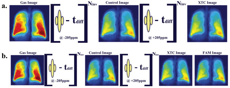
(a) At lower magnetic field three images are collected, where Gas and Control are separated by 180° pulses applied off-resonance, while the pulses between Control and XTC images are applied at dissolved state xenon frequency. The first two images are used for calibration purposes, and the last two provide 2D map of the fractional gas transport F. At 0.2T the loading of the coil did not change its Q significantly, allowing B₁ calibrations be performed independently. (b) At higher magnetic fields the rf coils are sensitive to the load, making it essential to implement a B₁ calibration routine for each run. We collected four 3D gradient echo images, the 1^st pair of images are used as before for calibration of other attenuation sources, 2^nd and 3^rd images to estimate F, and last two to obtain the B₁ distribution or Flip Angle Map (FAM). Performing all calibrations during the same breath-hold avoids image registration and lung volume control issues.

Table 3.

Pulse Sequence Parameters

Field Strength [T]	0.2	3
Data Matrix	64×32	32×32×8
TE [ms]	5.3	0.9
TR [ms]	24	2.1
Diffusion Time [ms]	62	20/44/62
Flip Angles (1st, 2nd, 3rd images) [degrees]	4, 4, 12	3, 3, 8
Inversion/Saturation pulses	44	110/56/44
FOV [mm]	300	300
Resolution (after zero filling) [mm]	2.4×4.7	5×5×10
Total Acquisition Time [s]	13	9.8

At 3T we collected 3D GRE images instead of 2D projections as the pulse sequences are faster at higher field and we could afford to collect full 3D data set in less time than the in vivo T₁. Further, the 3T scans were performed at a later time than the 0.2T scans and by that time we realized that only XTC with saturation pulses could be used to obtain S_A/V_Gas information. Therefore, at 3T we used saturation pulses instead of inversion pulses to create XTC weighting. Later we changed the protocol to collect four 3D GRE images with the first three images separated by saturation (90°) pulses applied at ±205 ppm from the gas phase (Figure 1b), while the last image served for estimation of B₁ distribution. With this, we evaluated the necessity of a pixel-wise B₁ distribution correction for the cases of sequential and centric encoding k-space acquisition (see Data Analysis for details). Similar to 0.2T runs, the first two images had the same flip angle, while that for the third one was higher. For the fourth image we used the same flip angle as in the third for the sake of simplicity. Similar to 0.2T runs, SNR optimization provided the flip angles for 3T runs (see Table 3 for the pulse sequence parameters). The raw data were zero-filled by a factor of 2 in all dimensions and then Fourier transformed, resulting in an apparent 5×5×10mm³ voxel size. To match the protocol implemented at 0.2T we used 44 saturation pulses for t_diff = 62ms run, while the number of saturation pulses for t_diff = 20 and 44ms was calculated to be such that attenuation due to F would match that of 62ms. This was done as follows: if $R_{t_{\mathit{diff}}}^{\mathit{Depol}}$ is the attenuation due to gas transfer for a particular diffusion time, then from $F\left(t_{\mathit{diff}}\right)=1-\sqrt[n]{R_{t_{\mathit{diff}}}^{\mathit{Depol}}}$ (n is the number of contrast generating pulses (14)) it follows that:

$$n\left(t_{\mathit{diff}}=20\text{or}44ms\right)=n\left(t_{\mathit{diff}}=62ms\right)·\mathit{Log}\left[\frac{1-F\left(62ms\right)}{1-F\left(20or44ms\right)}\right]$$ [1]

In these calculations we used the values of F previously measured with CSSR on the same subject at the same lung volume. The resulting number of saturation pulses used was 110/56 for 20/44ms diffusion times, respectively.

The zero offsets on F̄ were checked in experiments on phantoms, where there is no gas transfer into a dissolved state. A number of phantom experiments were performed at both field strengths. These experiments were analyzed in a manner identical to the human subject experiments.

RF pulses and Flip Angle Calibrations

The xenon spectrum in the lungs consists of a gas peak (at 0 ppm), and two dissolved state peaks: erythrocytes and non-blood tissue and plasma located at ~ 205ppm (~0.5kHz at 0.2T and ~7kHz at 3T) and spans over ~10ppm (~25Hz at 0.2T and ~340Hz at 3T). When exciting the dissolved state, the gas phase should be minimally disturbed, as the magnetization is non-renewable. This is imperative at 0.2T since the frequency separation between the phases is small. To address this, we numerically constructed a 3-lobe RF pulse shape with a trapezoidal spectrum such that when the dissolved state is inverted using a 10ms long pulse with a bandwidth of 100Hz, the gas phase experiences an excitation of less than 1°. Since the separation between the two phases at 3T is much larger, this did not pose a problem and a 0.75ms rectangular RF pulse shape was used. Also, as the bandwidth of this pulse is over 1.3kHz, it excited both dissolved state peaks.

At low field we performed flip angle calibrations on a number of phantoms filled with hyperpolarized xenon and in vivo for most of the subjects studied (five out of eight) to verify that sample loading of the coil is not significant. Standard techniques for hyperpolarized gases were employed, where a number of consecutive free induction decay signals are acquired, each followed by a set of spoiler gradients to de-phase any residual transverse magnetization prior to the next RF pulse. The data were fit to S_n = S₁ cosⁿ⁻¹(α), where α is the flip angle, S_n and S₁ are the n^th and initial signals, respectively, and n is the number of repetitions. TR (0.25s) was kept very short compared to T₁ of the gas (40–120 min in phantoms and 16 sec in vivo) to mitigate the longitudinal relaxation effects. The peripheral portion of the lungs is located close to the coil windings where the RF field is inhomogeneous, therefore the spatial distribution of the B₁ field was also investigated. We used the same approach as above and collected FIDs on a small gas cell on a 5-by-5 grid over the FOV. Since B₁ distribution is a slowly changing function of a position, we interpolated the data to the SB-XTC data matrix size. Then the images collected in the SB-XTC runs were pixel-wise corrected for B₁ distribution.

At high field, however, the coil is affected by the sample loading. We used two methods to acquire B₁ maps for calibrations. First, during a separate breath-hold prior to the actual SB-XTC experiment we collected 6 low resolution 3D GRE images with the same flip angle but different delay times between the images (we used 0, 8, 6, 4 and 2sec delay times). We used this data set to fit on a pixel-by-pixel basis S_n = S₁ cos^N*(n−1)(α)·e^−t/T₁, where α is the flip angle, S₁ and S_n are the pixel signals in the 1^st and n^th images, respectively, N and n are the number of phase encodings in an image and number of images, respectively. We obtained flip angle and T₁ (not used here) distributions from the fit. Further, we interpolated the B₁ map to the SB-XTC data size and used it in a pixel-wise flip angle correction outlined in Data Analysis (Eqn. 13a). In the second approach, B₁ map acquisition was incorporated into the SB-XTC experiment, thus avoiding any registration and lung volume matching issues. Later we also implemented 4-image SB-XTC with centric phase encoding to estimate whether B₁ distribution correction in this is dispensable as suggested by theoretical considerations (see Data Analysis for details). We compared F̄’s calculated with and without B₁ corrections applied.

Data Analysis

In SB-XTC the decay of the gas phase magnetization occurs due to three main mechanisms:diffusive gas transport from gas to dissolved phase, RF depletion and T₁ decay. Let S₁,S₂,S₃ and S₄ be pixel signal intensities for consecutively acquired images during a breath-hold (Figure 1). If S₀ represents the initial signal from gaseous xenon, N is the number of phase encoding lines in an image, TR is the repetition time and α_i is the flip angle used for the i^th image, then for the signal intensity at k=0 in the images, we can write:

$$\begin{array}{l}{S}_1=\{\begin{array}{ll}{S}_0·{\mathit{cos}}^{\frac{N}{2}}\left({\alpha }_1\right)·e^{-\frac{N}{2}·\frac{TR}{T_1}}·\mathit{sin}\left({\alpha }_1\right),\hfill & if\mathit{sequential}\mathit{encoding}\hfill \\ S_0·\mathit{sin}\left({\alpha }_1\right),\hfill & if\mathit{centric}\mathit{encoding}\hfill \end{array}\\ S_2=\{\begin{array}{ll}{S}_1·{\mathit{cos}}^{\frac{N}{2}}\left({\alpha }_1\right)·{\mathit{cos}}^{\frac{N}{2}}\left({\alpha }_2\right)·e^{-\left(\frac{N}{2}+\frac{N}{2}\right)·\frac{TR}{T_1}}·\mathit{sin}\left({\alpha }_2\right)·R_{\mathit{XTC}}^{-},\hfill & if\mathit{sequential}\mathit{encoding}\hfill \\ S_1·{\mathit{cos}}^N\left({\alpha }_1\right)·e^{-N·\frac{TR}{T_1}}·\mathit{sin}\left({\alpha }_2\right)·R_{\mathit{XTC}}^{-},\hfill & if\mathit{centric}\mathit{encoding}\hfill \end{array}\\ S_3=\{\begin{array}{ll}{S}_2·{\mathit{cos}}^{\frac{N}{2}}\left({\alpha }_2\right)·{\mathit{cos}}^{\frac{N}{2}}\left({\alpha }_3\right)·e^{-\left(\frac{N}{2}+\frac{N}{2}\right)·\frac{TR}{T_1}}·\mathit{sin}\left({\alpha }_3\right)·R_{\mathit{XTC}}^{+},\hfill & if\mathit{sequential}\mathit{encoding}\hfill \\ S_2·{\mathit{cos}}^N\left({\alpha }_2\right)·e^{-N\frac{TR}{T_1}}·\mathit{sin}\left({\alpha }_3\right)·R_{\mathit{XTC}}^{+},\hfill & if\mathit{centric}\mathit{encoding}\hfill \end{array}\\ S_4=\{\begin{array}{ll}{S}_3·{\mathit{cos}}^{\frac{N}{2}}\left({\alpha }_3\right)·{\mathit{cos}}^{\frac{N}{2}}\left({\alpha }_4\right)·e^{-\left(\frac{N}{2}+\frac{N}{2}\right)·\frac{TR}{T_1}}·\mathit{sin}\left({\alpha }_4\right),\hfill & if\mathit{sequential}\mathit{encoding}\hfill \\ S_3·{\mathit{cos}}^N\left({\alpha }_3\right)·e^{-N·\frac{TR}{T_1}}·\mathit{sin}\left({\alpha }_4\right),\hfill & if\mathit{centric}\mathit{encoding}\hfill \end{array}\end{array}$$ [2]

Here $R_{\mathit{XTC}}^{-}$ and $R_{\mathit{XTC}}^{+}$ are the total signal attenuations experienced during the XTC generating intervals between images 1–2 and 2–3, respectively (Figure 1). Each of them has a contribution from the T₁ relaxation denoted $R_{\mathit{XTC}}^{T_1}$ and from the effect the contrast generating rf pulses have on the gas signal $R_{\mathit{XTC}}^{rf}$ (although these pulses are applied at ∓205ppm, there still could be some, albeit small, excitation at the gas frequency); $R_{\mathit{XTC}}^{\mathit{Depol}}$ is the attenuation of the signal due to the pulses applied at the dissolved state frequency (+205ppm) that invert/saturate the dissolved state signal:

$$R_{\mathit{XTC}}^{-}=R_{\mathit{XTC}}^{-,rf}·R_{\mathit{XTC}}^{-,T_1}\text{and}{R}_{\mathit{XTC}}^{+}=R_{\mathit{XTC}}^{+,rf}·R_{\mathit{XTC}}^{+,T_1}·R_{\mathit{XTC}}^{\mathit{Depol}}$$ [3]

The relaxation effects will be the same for both cases since the same number of pulses with the same diffusion time were applied at + and − 205ppm: $R_{\mathit{XTC}}^{-,T_1}=R_{\mathit{XTC}}^{+,T_1}\equiv R_{\mathit{XTC}}^{T_1}$ denotes this T₁ relaxation contribution. Further, since the rf pulses applied to generate the contrast have a symmetric frequency profile, they will affect the gas phase ±205ppm away identically: $R_{\mathit{XTC}}^{-,rf}=R_{\mathit{XTC}}^{+,rf}\equiv R_{\mathit{XTC}}^{rf}$. Hence we obtain:

$$R_{\mathit{XTC}}^{+}=R_{\mathit{XTC}}^{rf}·R_{\mathit{XTC}}^{T_1}·R_{\mathit{XTC}}^{\mathit{Depol}}=R_{\mathit{XTC}}^{-}·R_{\mathit{XTC}}^{\mathit{Depol}}$$ [4]

Let us introduce the following parameters:

$$R_{T_1}=e^{-N\frac{TR}{T_1}}\text{and}{R}_{{\alpha }_i}={\mathit{cos}}^m\left({\alpha }_{i-1}\right)·{\mathit{cos}}^{N-m}\left({\alpha }_i\right)·\mathit{sin}\left({\alpha }_i\right)$$ [5]

here i=1, 2, 3, 4 is the image number, N is the number of phase encoding lines in an image, and we define α₀ = 0; further, let us define m as

$$m=\{\begin{array}{ll}\frac{N}{2},\hfill & if\mathit{sequential}\hfill \\ N,\hfill & if\mathit{centric}\hfill \end{array}$$ [6]

After plugging Eqns. [4–6] back into [2], the image intensities become:

$$\begin{array}{ll}{S}_1=\{\begin{array}{l}{S}_0·R_{{\alpha }_1}·\sqrt{R_{T_1}},\hfill \\ S_0·R_{{\alpha }_1},\hfill \end{array}\hfill & \begin{array}{l}\text{if}\text{sequential}\text{encoding}\\ \text{if}\text{centric}\text{encoding}\end{array}\hfill \\ S_2=S_1·R_{{\alpha }_2}·R_{T_1}·R_{\mathit{XTC}}^{rf}·R_{\mathit{XTC}}^{T_1},\hfill & \text{independent}\text{of}\text{encoding}\hfill \\ S_3=S_2·R_{{\alpha }_3}·R_{T_1}·R_{\mathit{XTC}}^{rf}·R_{\mathit{XTC}}^{T_1}·R_{\mathit{XTC}}^{\mathit{Depol}},\hfill & \text{independent}\text{of}\text{encoding}\hfill \\ S_4=S_3·R_{{\alpha }_4}·R_{T_1},\hfill & \text{independent}\text{of}\text{encoding}\hfill \end{array}$$ [7]

Then for $R_{\mathit{XTC}}^{\mathit{Depol}}$ we have

$$R_{\mathit{XTC}}^{\mathit{Depol}}=\frac{S_3}{S_2·R_{{\alpha }_3}·R_{T_1}·R_{\mathit{XTC}}^{rf}·R_{\mathit{XTC}}^{T_1}}$$ [8]

and using

$$R_{T_1}·R_{\mathit{XTC}}^{rf}·R_{\mathit{XTC}}^{T_1}=\frac{S_2}{S_1·R_{\alpha 2}}$$ [9]

we get:

$$R_{\mathit{XTC}}^{\mathit{Depol}}=\frac{S_3}{S_2}·\frac{S_1}{S_2}·\frac{R_{{\alpha }_2}}{R_{{\alpha }_3}}$$ [10]

The flip angle maps were obtained from [2] with α₃= α₄ and neglecting T₁ relaxation during the image acquisition (T_A <0.5s≪T₁ = 16s):

$${\beta }_{\mathit{meas}}={\mathit{cos}}^{-1}\left(\sqrt[N]{R_{{\alpha }_4}}\right)={\mathit{cos}}^{-1}\left(\sqrt[N]{\frac{S_4}{S_3}}\right)$$ [11]

In three-image experiments at 0.2T and 3T we set α₁= α₂ ≡ α and α₃ ≡ β and used a sequential phase encoding trajectory, resulting in

$$R_{\mathit{XTC}}^{\mathit{Depol}}=\frac{S_3}{S_2}·\frac{S_1}{S_2}·\frac{{\mathit{cos}}^{\frac{N}{2}}\left(\alpha \right)}{{\mathit{cos}}^{\frac{N}{2}}\left(\beta \right)}·\frac{\mathit{sin}\left(\alpha \right)}{\mathit{sin}\left(\beta \right)}$$ [12a]

while in four-image experiments at 3T we used centric encoding trajectory and α₁= α₂ ≡ α and α₃= α₄ ≡ β:

$$R_{\mathit{XTC}}^{\mathit{Depol}}=\frac{S_3}{S_2}·\frac{S_1}{S_2}·\frac{\mathit{sin}\left(\alpha \right)}{\mathit{sin}\left(\beta \right)}$$ [12b]

Here N is the number of phase encoding steps used in the images. With flip angle correction implemented on a pixel-by-pixel basis [12 a–b] become:

$$R_{\mathit{XTC}}^{\mathit{Depol}}=\frac{S_3}{S_2}·\frac{S_1}{S_2}·\frac{{\mathit{cos}}^{\frac{N}{2}}\left(\frac{\alpha }{\beta }{\beta }_{\mathit{meas}}\right)}{{\mathit{cos}}^{\frac{N}{2}}\left({\beta }_{\mathit{meas}}\right)}·\frac{\mathit{sin}\left(\frac{\alpha }{\beta }{\beta }_{\mathit{meas}}\right)}{\mathit{sin}\left({\beta }_{\mathit{meas}}\right)}$$ [13a]

$$R_{\mathit{XTC}}^{\mathit{Depol}}=\frac{S_3}{S_2}·\frac{S_1}{S_2}·\frac{\mathit{sin}\left(\frac{\alpha }{\beta }{\beta }_{\mathit{meas}}\right)}{\mathit{sin}\left({\beta }_{\mathit{meas}}\right)}$$ [13b]

The presence of the cos^N/2 factor in [13a] suggests that the sequential encoding is more sensitive to inhomogeneous B₁ fields.

Finally, for a voxel the fractional gas transport F, which at short diffusion times represents a parameter proportional to the locally averaged functional S_A/V_Gas, is (14)

$$F\left(t_{\mathit{diff}}\right)=1-\sqrt[n]{R_{\mathit{XTC}}^{\mathit{Depol}}}$$ [14]

with t_diff being the time allowed for diffusion and n - the number of inversion/saturation pulses. Performing analysis in this fashion we mapped the fractional gas transport distribution. It should be reiterated here that because at 0.2T we used inversion pulses as opposed to saturation pulses used at 3T, the values of F measured for the same t_diff should be different (16). We then calculated the mean (F̄)and the standard deviation (σ_total) of F, with the latter being a measure of heterogeneity in the fractional gas transport. We also averaged F in the right/left dimension to obtain the dependence of F on the cranial/caudal axis. For short diffusion times (8,9)

$$F\left(t_{\mathit{diff}}<100ms\right)=F_0+\lambda ·\frac{S_A}{V_{\mathit{Gas}}}·\sqrt{\frac{4D}{\pi }·t_{\mathit{diff}}}$$ [15]

where λ is the partition coefficient, D is xenon diffusion coefficient in tissue and F₀ is an offset (see (8) for details). By measuring F at different diffusion times we estimated S_A/V_Gas from the slope of $Fvs.\sqrt{t_{\mathit{diff}}}$.

Heterogeneity Analysis

The heterogeneity in measured F(σ_total) has two sources: the physiological heterogeneity (σ_physiol) of the lungs and the system noise (σ_noise). In order to separate the two, we estimated the error in F due to the noise only in the images by obtaining additional data sets (sham background runs, Table 2), before and/or after each SB-XTC experiment, in which the subject inhaled air only. If σ₁, σ₂ and σ₃ are the standard deviations of the noise calculated from corresponding images we could write

$$\overline{F}\left({\overline{S}}_1,{\overline{S}}_2,{\overline{S}}_3\right)\pm {\sigma }_{\mathit{total}}=1-\sqrt[n]{\frac{{\overline{S}}_1\pm {\sigma }_1}{{\overline{S}}_2\pm {\sigma }_2}·\frac{{\overline{S}}_3\pm {\sigma }_3}{{\overline{S}}_2\pm {\sigma }_2}·\frac{{\overline{R}}_{{\alpha }_2}}{{\overline{R}}_{{\alpha }_3}}}$$ [16]

Then under an assumption that noise adds incoherently we can estimate and separate the contribution of the noise in the images to the total uncertainty in F̄, thus providing a measure of heterogeneity in F̄ due to only physiological sources:

$${\sigma }_{\mathit{total}}=\sqrt{{\sigma }_{\mathit{physiol}}^2+{\sigma }_{\mathit{noise}}^2}$$ [17]

In order to do that we need to propagate the error in F̄ due to σ₁, σ₂ and σ₃:

$${\sigma }_{\mathit{noise}}^2={\left(\frac{\partial \overline{F}}{\partial {\overline{S}}_1}·{\sigma }_1\right)}^2+{\left(\frac{\partial \overline{F}}{\partial {\overline{S}}_2}·{\sigma }_2\right)}^2+{\left(\frac{\partial \overline{F}}{\partial {\overline{S}}_3}·{\sigma }_3\right)}^2$$ [18]

For the derivatives in each element of the sum we have

$$\begin{array}{l}\frac{\partial \overline{F}}{\partial {\overline{S}}_1}=-\frac{1}{n}·\frac{1}{S_1}·{\left(\frac{{\overline{S}}_1}{{\overline{S}}_2}·\frac{{\overline{S}}_3}{{\overline{S}}_2}·\frac{{\overline{R}}_{{\alpha }_2}}{{\overline{R}}_{{\alpha }_3}}\right)}^{\frac{1}{n}};\\ \frac{\partial \overline{F}}{\partial {\overline{S}}_2}=+\frac{2}{n}·\frac{1}{S_2}·{\left(\frac{{\overline{S}}_1}{{\overline{S}}_2}·\frac{{\overline{S}}_3}{{\overline{S}}_2}·\frac{{\overline{R}}_{{\alpha }_2}}{{\overline{R}}_{{\alpha }_3}}\right)}^{\frac{1}{n}};\\ \frac{\partial \overline{F}}{\partial {\overline{S}}_3}=-\frac{1}{n}·\frac{1}{S_3}·{\left(\frac{{\overline{S}}_1}{{\overline{S}}_2}·\frac{{\overline{S}}_3}{{\overline{S}}_2}·\frac{{\overline{R}}_{{\alpha }_2}}{{\overline{R}}_{{\alpha }_3}}\right)}^{\frac{1}{n}};\end{array}$$ [19]

Hence we get

$${\sigma }_{\mathit{noise}}=\frac{1}{n}·\sqrt[n]{\frac{{\overline{S}}_1}{{\overline{S}}_2}·\frac{{\overline{S}}_3}{{\overline{S}}_2}·\frac{{\overline{R}}_{{\alpha }_2}}{{\overline{R}}_{{\alpha }_3}}}·\sqrt{{\left(\frac{{\sigma }_1}{{\overline{S}}_1}\right)}^2+4·{\left(\frac{{\sigma }_2}{{\overline{S}}_2}\right)}^2+{\left(\frac{{\sigma }_3}{{\overline{S}}_3}\right)}^2}$$ [20]

and σ_physiol will be

$${\sigma }_{\mathit{physiol}}=\sqrt{{\sigma }_{\mathit{total}}^2-{\sigma }_{\mathit{noise}}^2}$$ [21]

Results

At 0.2T, the variation between the flip angles measured in phantoms and subjects was ~3%. This was taken as sufficient evidence that the loading of the coil by the subjects is insignificant and we concluded that different subjects would not affect the B₁ distribution within the field of view and that a single map derived from a phantom would be valid for all human subjects. When mapping the B₁ field at 0.2T, a slight asymmetry was observed between the sides of the coil. Also, there was a significant variation of the flip angle within the field of view (Figure 2(a)), which in light of sequentially encoded trajectory (Eqn. 13a) necessitated a pixel-wise B₁ correction of the data. The results of the flip angle distribution mapping at 3T are shown in Figure 2(b).

Figure 2.

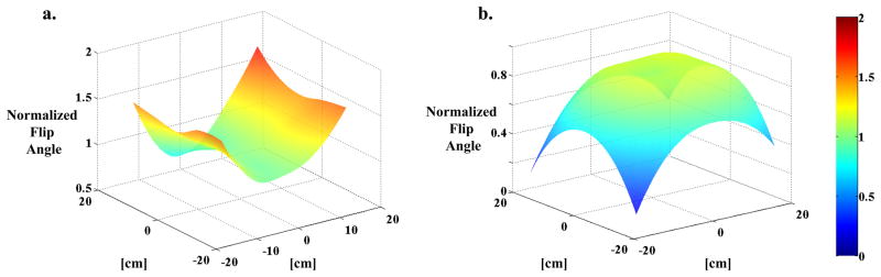
Flip Angle Maps. (a) FAM collected at 0.2T using a small spherical cell filled with hyperpolarized xenon gas. The data is interpolated to a larger matrix size to match the size of SB-XTC data matrix, and normalized to the flip angle setting used in the run. (b) FAM collected in vivo during a breath-hold as part of the SB-XTC experiment. The map is calculated using images #3 and 4, following the routine outlined in data analysis. Again, the values are normalized to the flip angle setting used in the run.

The SB-XTC sequence was validated via a number of experiments at both field strengths performed on xenon gas phantoms in the absence of gas exchange: F̄_expected= 0. The mean value of F̄ from six phantom experiments at 0.2T is 0.01%, while the standard deviation between them is 0.02%, which is well below the values seen in the subjects and is negligible. However, these were found only after correcting for the B₁ distribution (for example, in one of the cases before the correction F̄= −0.5±0.1%, which in absolute value is comparable with the amount of gas transport one expects to measure in vivo, while after correction F̄= 0.03±0.08%,). The corresponding numbers from the four experiments performed at 3T are: mean=0.01%, standard deviation =0.01%.

For SB-XTC studies at 3T we selected t_diff = 20/44/62ms, all within the $\sqrt{t_{\mathit{diff}}}$ behavior region. These diffusion time values make our measurements sensitive to regions 3.5 7μm thick, which would include tissue and vasculature. Based on F values measured with CSSR for times near 62ms we predicted that 30 to 50 inversion pulses would produce sufficient contrast for the measurement. The further optimization of the number of inversion pulses in a series of in vivo experiments (Figure 3) provided 44 as the optimal number of inversion pulses that balanced signal attenuation and SNR of the measurement. The error bars at the limits of the range are expected to be relatively large: for a low number of inversions, the resulting change in the signal due to F will be small and therefore subject to a large variance; similarly, for a large number of inversions, the large attenuation would result in poor SNR for the XTC image.

Figure 3.

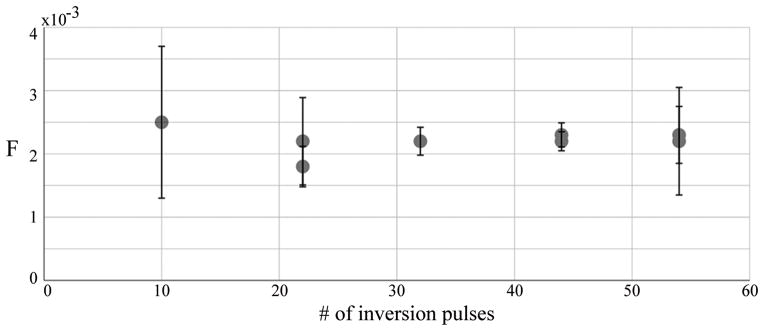
<F(t)> as a function of the number of inversion pulses. Based on these results, 44 inversion pulses were used in the studies.

A set of sample images from an SB-XTC experiment is presented in Figure 4: (a) presents the data set from SB-XTC run with 20 ms diffusion time (six of 12 slices are presented), while (b) shows four images from one of the slices for all three diffusion times. Following the outlined data analysis routine, we produced a spatial map of F(t_diff) in the lungs: Figure 5(a–c) displays the F-maps calculated for each of three diffusion times. Note that if the effect of the inversion/saturation RF pulse (applied at −205 ppm) on the gas signal is well known (either correctable or negligible) then one can translate $R_{\mathit{XTC}}^{-}$ into a map of the local oxygen partial pressure (19).

Figure 4.

Sample of 3D SB-XTC images collected at high field. (a) Data from the 20ms delay time run. Six out of twelve slices are presented to preserve space. Four images in each row correspond to Gas image (collected before the application of the saturation pulses), Control image (collected after the application of the saturation pulses at −205ppm), XTC image (collected after the application of the saturation pulses at +205ppm), and finally FAM image collected with the same flip angle as the XTC image. (b) A single slice data (from the four consecutive images) corresponding to three different delay times are presented for comparison. To minimize differences in the images, the subject remained inside the scanner between the experiments, while bags with gas mixture were prepared (~5min).

Figure 5.

F-maps calculated for diffusion times of (a) 20ms, (b) 44ms and (c) 62ms. One curious feature of the data is the change in the gradient direction of the F values from anterior to posterior slices: in 20ms F-maps the anterior slices have lower F compared to posterior, as expected from gravitational dependence. However this gradient direction is reversed in 44 and 62ms F-maps. This could be explained by effect of different thickness contributions to F₀ offset.

As a function of lung volume (VL) alveolar surface area increases slower than the gas volume (26). Therefore S_A/V_Gas and hence F are expected to decrease as VL increases. Additionally, as VL approaches TLC, the regional heterogeneity is known to decrease (27). Depolarization maps at three VL’s and their corresponding histograms in Figure 6(a–d) demonstrate both features: not only the mean value of F but also the width of the distribution has decreased with the increasing VL. Similar behavior was observed in all subjects: Figure 7 summarizes the dependence of the mean fractional gas transport and the calculated physiological heterogeneity on the lung volume. The red trend line in (a) is the fit of the data to a power function. This particular functional form was selected based on earlier histological works by Gil et al. (26), Weibel (28) and Thurlbeck (29). The fit revealed the following relationship: $F=0.8·V_{\mathit{Gas}}^{-0.9}$, R²= 0.8.

Figure 6.

Fractional gas transport F(62ms) at three different lung volumes (VL) with corresponding histograms. Data presented here are from two subjects. (a) F-map at 18% TLC (near RV, HS7), mean value − <F> = 3.74%, σ_Physiol = 1.15%; (b) F-map at 40% TLC (HS1), mean value − <F> = 1.5%, σ_Physiol = 0.4%; (c) F-map at 80% TLC (HS1), mean value − <F> = 0.77%, σ_Physiol = 0.37%. Note that although there is a substantial difference in the lung volumes at 18, 40 and 80% of TLC, it is hard to appreciate this volume difference in the maps: since these are maps based on 2D projection images, they are missing the thickness information of the lungs, thus present misleading feel of comparable lung volumes. The important message from this figure is in the color differences between the F-maps, as well as the color distribution in each of the maps. (d) histograms corresponding to the F-maps (green – 18% TLC (a), blue – 40% TLC (b), and red – 80% TLC (c)).

Figure 7.

Lung volume dependence of the mean fractional gas transport <F> (a) and physiological heterogeneity σ_physiol (b), both plotted on a Log-Log scale. All data are from 0.2T only. To enable intersubject comparison, the lung volumes are normalized to TLC of each subject. <F> from all subjects is in good agreement within the error, which is represented here by the contribution of the noise to the width of the fractional gas transport distribution. In most cases the largest contribution to the width of <F> distribution comes from the physiological heterogeneity.

Although the data were collected in the supine position, at lower VL’s we observed higher F̄ values at the bases compared to the apices for all subjects (Figure 8a). Closer to TLC these differences in the cranio-caudal direction evened out in all subjects (Figure 8b, sample plot from one subject).

Figure 8.

(a) In all runs with healthy volunteers at lung volumes near FRC we observed positive gradient in Apex-to-Base direction. (b) As lung volumes increase approaching TLC the Apex-to-Base gradient disappears. Presented is a sample data from one of the subjects at two lung volumes: the red triangles correspond to higher lung volume while blue circles correspond to lower lung volume experiments.

At 3T we obtained 3D distributions of F for three different diffusion times (20/44/62ms) in the same subject after inhalation of similar volumes of gas. Figure 5 shows the F-maps with the following global mean values and standard deviations: F̄(20ms)= 0.2±0.1%, F̄ (44ms)= 0.7±0.3% and F̄(62ms)= 1±0.4%. Regional S_A/V_Gas distribution (Figure 9a) was obtained by pixel-wise fitting the F data to Eqn. [15] after the F-maps were registered using Matlab’s built-in image registration tools (for sample pixel fits see Figure 9b). This estimation of S_A/V_Gas is based on partition coefficient λ= 0.1 (30) and diffusion coefficient D = 3.8·10⁻⁶ cm²/s of xenon in the tissue (25). During the fitting routine, F₀ was constrained to be non-negative asF₀<0 does not carry a real physical meaning. The global mean value and standard deviation for S_A/V_Gas obtained from the fits are 89cm⁻¹ and 30cm⁻¹.

Figure 9.

(a) The S/V-map in units of inverse cm calculated from a pixel-wise linear model fit of F to √t_diff (see data analysis). The global mean value for S/V is 89±30 cm⁻¹ (mean ± standard deviation). (b) Representative voxel-wise fits of F to the short-time model from four different voxels measured at three diffusion times.

Figure 10 shows the results of the comparison of mean values of F calculated with and without B₁ distribution corrections. Also, to independently evaluate the significance of the correction we used Student’s t-test which, at p= 0.05, failed to reject the null hypothesis that the difference between the two data sets (F values calculated from centric data with and without correction) has a mean of zero. A similar test performed on the sequentially encoded data displayed significant difference at this level.

Figure 10.

Comparison of F obtained from images with centric (3T only) and sequential encoding of k-space. It is evident from the data that in the case of centrically encoded k-space, the B₁ correction of the data does not significantly affect the value of F and might be omitted (circles in the plot). However, in the case of sequentially encoded k-space the implementation of the B₁ correction (preferably during the same breathhold as in the case of four-image SB-XTC) might be necessary (squares and rhombi in the plot), even in the case of small variation in the flip angle (less than 10% variation in the flip angle over the FOV, 3T data).

Discussion

XTC is a powerful technique capable of extracting information on regional lung function. The presented modifications to the technique avoid complications associated with image registration and VL control, allowing studies in conscious humans. Our earlier observation that XTC can yield results similar to CSSR when using 90° RF pulses allows its use to obtain S_A/V_Gas maps (10).

SB-XTC was implemented and tested on several levels. First, the sequence was calibrated on phantoms containing no dissolved xenon, highlighting the necessity of B₁ correction: “zero” values were obtained only after the pixel-wise correction for B₁ distribution. Next, the technique was numerically optimized to predict the experimental parameters and then further optimized through a series of experiments with variable numbers of inversion pulses that provided consistent F̄ values under similar conditions. In all subjects we performed repeat measurements at one of the lung volumes. Figures 3 and 7a demonstrate high degree of reproducibility from the spread of the data in repeat runs, which established the technique’s robustness.

The diffusion times (20/44/62ms) for the experiments were chosen below the time (100ms) at which F(t_diff) deviates from the established short time $\sqrt{t_{\mathit{diff}}}$ behavior (8). The measurements presented here are consistent with the choice of t_diff. The xenon partition coefficient in blood is between 0.107 and 0.123, while in saline it is 0.096 (30), which led to the choice of the intermediate value of 0.1 for the tissue. Lung tissue constitutes ~20% of the total VL near FRC (31), therefore when the tissue is saturated with xenon its fraction in it is ~2%. Near FRC the highest measured F̄₁₈₀(62ms)= 2.4% per inversion pulse(note F̄₁₈₀ ≈ 2· F̄₉₀)and F̄₉₀(62ms)= 1% per saturation pulse (Table 2), both well below the estimated 2%. This supports our interpretation of F(t_diff) reflecting the functional surface area.

With SB-XTC we observed that F̄, and hence $\overline{S_A/V_{\mathit{Gas}}}$ decreased with the increase of VL for all subjects (Figure 7a). This is in agreement with classic histological studies of Gil et al. (26), Weibel (28), Thurlbeck (29) on fixed human lungs, in vivo animal studies by Ruppert et al. (15) and very recently by Hajari et al. (32). However, in their studies on human lungs Weibel and Thurlbeck both obtained dependence of S_A on V_Gas of the form $\frac{S_A}{V_{\mathit{Gas}}}\propto V_{\mathit{Gas}}^{-\frac{1}{3}}$ corresponding to balloon-like reduction of alveolar size while Gil in his study on rabbit lungs obtained $\frac{S_A}{V_{\mathit{Gas}}}\propto V_{\mathit{Gas}}^{-0.67}$ for air-filled and $\frac{S_A}{V_{\mathit{Gas}}}\propto V_{\mathit{Gas}}^{-0.42}$ for saline-filled lungs. From our in vivo measurements we get $\frac{S_A}{V_{\mathit{Gas}}}\propto V_{\mathit{Gas}}^{-0.93}$ (the trendline in Figure 7a), thus suggesting crumpling of the alveolar surface or anisotropic accordion-like deformations described by Gil and co-authors (26). However, we cannot yet draw a firm conclusion on the lung volume dependence of S_A/V_Gas: although our measurements were done in the $\sqrt{t_{\mathit{diff}}}$ regime, diffusion times(20/40/62ms)are still relatively long so that thin parts of the parenchyma will have been already saturated, thus rendering these measurements “blind” to changes in some parts of the parenchymal surface. Since the thinnest parts of the parenchyma are ~0.5μm the “true” S_A can only be measured with t_diff <1ms, which is currently not feasible technically, and so the scaling issue must remain open.

In the upright posture and at lower VL’s the apices of a lung are more inflated than the basal portions (27), creating a gradient in the local S_A/V_Gas. Although our measurements were performed in supine subjects, such a trend was still observed in all subjects near FRC, and may reflect structural inhomogeneities along the apex-base axis, unrelated to gravitationally induced variations; or it could reflect residual structural gradients induced during wakefulness in the upright position. Further, it is widely accepted that in healthy volunteers lungs are more homogeneous at higher volumes (27), which in turn implies a marked decrease in any S_A/V_Gas gradient; our data echoes this behavior apex-base gradient in F disappeared at high VL and σ_physiol decreased with increase of VL.

Using Eqn. [15] the single time-point F-map measurements could be translated into S_A/V_Gas–maps (assuming F₀ = 0). However, since the parenchymal thickness is not uniform, some parts of the septum will have been saturated even after a short t_diff, which implies that S_A/V_Gas values would be underestimated. In order to properly estimate the pulmonary surface area multiple time-point measurements are necessary. At 3T we measured F-maps at three different diffusion time points, allowing for better estimation of S_A/V_Gas (Figure 9). The S_A/V_Gas values we report here vary from the previously reported values (10). The reason for this is that the global mean $\overline{S_A/V_{\mathit{Gas}}}=267\pm 62{cm}^{-1}$ reported earlier was estimated via averaging the pixel-by-pixel calculations of S_A/V_Gas from two time point measurements: $\frac{S_A}{V_{\mathit{Gas}}}=\frac{\left[F(62ms)-F\left(44ms\right)\right]/\left[\sqrt{62ms}-\sqrt{44ms}\right]}{\lambda \sqrt{4D/\pi }}$, which did not ensure a non-negative intercept. This however could overestimate the value of S_A/V_Gas. When we reanalyzed the data and forced the intercept to be non-negative (Figure 9b), we obtained $\overline{S_A/V_{\mathit{Gas}}}=109\pm 45{cm}^{-1}$, which is in an agreement with the data reported here.

We implemented SB-XTC with sequential and centric k-space trajectories. We showed that in the case of sequential encoding it is necessary to correct for the B₁ distribution within the field of view. At the same time, the use of centric phase encoding, given relatively uniform B₁ distribution, rendered the flip angle corrections unnecessary. Fundamentally in sequentially encoded experiments the cos^N/2(β) factor, unless corrected, skews the signal attenuation, thus affecting the value of F. It needs to be noted however, that here we corrected for the effect of the RF pulses used in the image acquisitions only and neglected the effect of imperfections of the saturation/inversion pulses.

Very recently Dregely et al. (18) implemented general SB-XTC approach (17) to collect two different diffusion time measurements during a single breath-hold. This extension of the technique to include more diffusion time measurements to obtain the local septal thickness along with surface area available for diffusion is one avenue by which a noninvasive assay is made that specifically differentiates the separate contributions of the septal area and thickness to the mean local tissue density (as can be measured with computed tomography). However, in such measurements one needs to be extremely careful with the choice of imaging protocol and parameters. As we have demonstrated in this study, if no explicit B₁ distribution correction is implemented one needs to use centric encoding to traverse the k-space. Further, since there is only a single control experiment for multiple diffusion times, one needs to ensure that the total time for XTC creation for both time points is the same, so that T₁ effect for both XTC parts is identical. And finally, since for different diffusion times the number of XTC RF pulses will be different, while the control part will match only one of these numbers, one has to ensure that the RF pulse applied at±208 ppm does not have any effect on the gas phase magnetization.

Further, measurements at longer diffusion times, when the full xenon uptake model must be used to describe the data, will allow estimation of parenchymal surface area, septal thickness, and capillary transit time, representing an important tool in the differential diagnosis and management of pulmonary diseases affecting each of those parameters. Initial steps have been taken by (i) comparing F̄ measured using SB-XTC spectroscopy with the values from direct CSSR measurements at several different diffusion times (8,33), (ii) studying these parameters globally in healthy subject and subjects with cronic obstructive pulmonary disease (COPD) and interstitial lung disease using CSSR (10), and (iii) comparing multiple time XTC generated regional parameters between healthy volunteers and patients with COPD and asthma (18).

A confounding issue for this study is its implementation at different field strengths with a wide range of parameters. This had to do with infrastructure changes beyond our control, such as decommissioning of the 0.2T scanner we used for the studies. However, this forced us to obtain F using different systems at different field strengths, and allowed us to obtain insight into one very important question: whether measurement of these important physiological parameters (F and S_A/V_Gas) is field dependent, namely whether susceptibility plays an important role in the measurements. In the earlier measurements at 0.2T where we expect susceptibility to be of minimal importance, we compared the slope K of $F\text{vs}.\sqrt{t_{\mathit{diff}}}$ obtained from spectroscopic SB-XTC (using inversion pulses, K_XTC) and CSSR (K_CSSR): K_XTC/K_CSSR = 2.5 (8). Measurements on the same subject presented here with F obtained using SB-XTC first with inversion pulses at 0.2T (F_0.2T) and then with saturation pulses (in which case results are comparable with CSSR data) at 3T (F_3T), show that (F_0.2/F_3T = 2.1. Further, Ruppert et al. (14) estimated that for long diffusion times F_XTC/F_CSSR = 2. This initial comparison is very encouraging as all these ratios are fairly close to each other. If susceptibility at 3T did play an important role in the value of F_3T measured, these ratios would not be similar. This data therefore provides initial evidence that measurement of F, and thus S/V, is field independent and can be compared across the field strengths.

In conclusion, we implemented SB-XTC at both low and high magnetic fields, obtained F-maps and physiological heterogeneity from eight volunteers to study lung volume dependence of F, thus S_A /V_Gas, and its homogeneity in vivo. We found that both the mean value and the heterogeneity of the fractional diffusive xenon transport F increased with the decreasing VL. A systematic regional increase in F in the lung bases was observed at lower VL’s in all volunteers. We obtained 3-dimentional F-maps in one subject at three different diffusion times within the validity regime of the $\sqrt{t_{\mathit{diff}}}$ behavior of F and estimated the local functional alveolar surface area per unit gas volume (with a mean ± standard deviation of $\overline{S_A/V_{\mathit{Gas}}}=89\pm 30{cm}^{-1}$). We showed that if centric k-space encoding is used, small variations in the B₁ over the field of view can be neglected, while in the case of sequential encoding, B₁ correction of the data is necessary.

References

- 1.Bouchiat M, Carver T, Varnum C. Nuclear Polarization in 3He Gas Induced by Optical Pumping and Dipolar Exchange. Phys Rev Lett. 1960;5(8):373–375. [Google Scholar]
- 2.Albert MS, Cates GD, Driehuys B, Happer W, Saam B, Springer CS, Wishnia A. Biological magnetic resonance imaging using laser-polarized 129Xe. Nature. 1994;370(6486):199–201. doi: 10.1038/370199a0. [DOI] [PubMed] [Google Scholar]
- 3.Driehuys B, Cates aGD, Miron E, Sauer K, Walter DK, Happer W. High-volume production of laser-polarized 129Xe. Appl Phys Lett. 1996;69(12):1668–1670. [Google Scholar]
- 4.Ruset I, Ketel S, Hersman F. Optical Pumping System Design for Large Production of Hyperpolarized 129Xe. Phys Rev Lett. 2006;96(5):53002. doi: 10.1103/PhysRevLett.96.053002. [DOI] [PubMed] [Google Scholar]
- 5.Mugler JP, Driehuys B, Brookeman JR, Cates GD, Berr SS, Bryant RG, Daniel TM, de Lange EE, Downs JH, Erickson CJ, Happer W, Hinton DP, Kassel NF, Maier T, Phillips CD, Saam BT, Sauer KL, Wagshul ME. MR imaging and spectroscopy using hyperpolarized 129Xe gas: preliminary human results. Magn Reson Med. 1997;37(6):809–815. doi: 10.1002/mrm.1910370602. [DOI] [PubMed] [Google Scholar]
- 6.Mansson S, Wolber J, Driehuys B, Wollmer P, Golman K. Characterization of diffusing capacity and perfusion of the rat lung in a lipopolysaccaride disease model using hyperpolarized 129Xe. Magn Reson Med. 2003;50(6):1170–1179. doi: 10.1002/mrm.10649. [DOI] [PubMed] [Google Scholar]
- 7.Driehuys B, Cofer G, Pollaro J, Mackel J, Hedlund L, Johnson G. Imaging alveolar-capillary gas transfer using hyperpolarized 129Xe MRI. Proc Natl Acad Sci USA. 2006;103(48):18278–18283. doi: 10.1073/pnas.0608458103. [DOI] [PMC free article] [PubMed] [Google Scholar]
- 8.Patz S, Muradian I, Hrovat MI, Ruset IC, Topulos G, Covrig SD, Frederick E, Hatabu H, Hersman FW, Butler JP. Human pulmonary imaging and spectroscopy with hyperpolarized 129Xe at 0.2T. Academic Radiology. 2008;15(6):713–727. doi: 10.1016/j.acra.2008.01.008. [DOI] [PMC free article] [PubMed] [Google Scholar]
- 9.Butler JP, Mair RW, Hoffmann D, Hrovat MI, Rogers RA, Topulos GP, Walsworth RL, Patz S. Measuring surface-area-to-volume ratios in soft porous materials using laser-polarized xenon interphase exchange nuclear magnetic resonance. Journal of physics Condensed matter. 2002;14(13):L297–304. doi: 10.1088/0953-8984/14/13/103. [DOI] [PMC free article] [PubMed] [Google Scholar]
- 10.Patz S, Muradyan I, Hrovat MI, Dabaghyan M, Washko GR, Hatabu H, Butler JP. Diffusion of hyperpolarized 129Xe in the lung: a simplified model of 129Xe septal uptake and experimental results. New Journal of Physics. 2011;13:015009. [Google Scholar]
- 11.Muradian I, Patz S, Butler J, Topulos G. Hyperpolarized 129Xe human pulmonary gas exchange with 3-point Dixon technique. Proceedings of ISMRM. 2006;14:1297. [Google Scholar]
- 12.Muradyan I. Thesis. 2007. Structural and Functional Pulmonary Imaging using Hyperpolarized 129Xe; pp. 1–223. (microfilm) [Google Scholar]
- 13.Mugler JP, Altes TA, Ruset IC, Dregely IM, Mata JF, Miller GW, Ketel S, Ketel J, Hersman FW, Ruppert K. Simultaneous magnetic resonance imaging of ventilation distribution and gas uptake in the human lung using hyperpolarized xenon-129. Proc Natl Acad Sci USA. 2010;107(50):21707–21712. doi: 10.1073/pnas.1011912107. [DOI] [PMC free article] [PubMed] [Google Scholar]
- 14.Ruppert K, Brookeman JR, Hagspiel KD, Mugler JP. Probing lung physiology with xenon polarization transfer contrast (XTC) Magn Reson Med. 2000;44(3):349–357. doi: 10.1002/1522-2594(200009)44:3<349::aid-mrm2>3.0.co;2-j. [DOI] [PubMed] [Google Scholar]
- 15.Ruppert K, Mata JF, Brookeman JR, Hagspiel KD, Mugler JP. Exploring lung function with hyperpolarized (129)Xe nuclear magnetic resonance. Magn Reson Med. 2004;51(4):676–687. doi: 10.1002/mrm.10736. [DOI] [PubMed] [Google Scholar]
- 16.Hrovat MI, Muradian I, Frederick E, Butler JP, Hatabu H, Patz S. Theoretical Model for XTC (Xenon Transfer Contrast) Experiments with Hyperpolarized 129Xe. Proceedings of ISMRM. 2010;18:2556. [Google Scholar]
- 17.Muradian I, Butler J, Hrovat M, Topulos G, Hersman E, Frederick E, Covrig S, Ruset I, Ketel S, Hersman W, Patz S. Human Regional Pulmonary Gas Exchange with Xenon Polarization Transfer (XTC) Proceedings of ISMRM. 2007;15:454. [Google Scholar]
- 18.Dregely I, Mugler JP, Ruset IC, Altes TA, Mata JF, Miller GW, Ketel J, Ketel S, Distelbrink J, Hersman FW, Ruppert K. Hyperpolarized Xenon-129 gas-exchange imaging of lung microstructure: First case studies in subjects with obstructive lung disease. J Magn Reson Imaging. 2011;33(5):1052–1062. doi: 10.1002/jmri.22533. [DOI] [PMC free article] [PubMed] [Google Scholar]
- 19.Patz S, Hersman FW, Muradian I, Hrovat MI, Ruset IC, Ketel S, Jacobson F, Topulos GP, Hatabu H, Butler JP. Hyperpolarized (129)Xe MRI: a viable functional lung imaging modality? European journal of radiology. 2007;64(3):335–344. doi: 10.1016/j.ejrad.2007.08.008. [DOI] [PMC free article] [PubMed] [Google Scholar]
- 20.Lindholm P, Lundgren CEG. The physiology and pathophysiology of human breath-hold diving. J Appl Physiol. 2009;106(1):284–292. doi: 10.1152/japplphysiol.90991.2008. [DOI] [PubMed] [Google Scholar]
- 21.Lindholm P, Norris CM, Braver JM, Jacobson F, Ferrigno M. A fluoroscopic and laryngoscopic study of glossopharyngeal insufflation and exsufflation. Respiratory physiology & neurobiology. 2009;167(2):189–194. doi: 10.1016/j.resp.2009.04.013. [DOI] [PubMed] [Google Scholar]
- 22.Muradyan I, Loring SH, Ferrigno M, Lindholm P, Topulos GP, Patz S, Butler JP. Inhalation heterogeneity from subresidual volumes in elite divers. Journal of Applied Physiology. 2010;109(6):1969. doi: 10.1152/japplphysiol.00953.2009. [DOI] [PMC free article] [PubMed] [Google Scholar]
- 23.Dregely IM, Wiggins GC, Ruset IC, Brackett JR, Ketel S, Distelbrink JH, Alagappan V, Mareyam A, Potthast A, Polimeni J, Wald LL, Ruppert K, Altes TA, JPM, Hersman FW. A 32 Channel Phased Array Lung Coil for Parallel Imaging with Hyperpolarized Xenon 129 at 3T. Proceedings of ISMRM. 2009;17:2203. [Google Scholar]
- 24.Hersman FW, Ruset IC, Ketel S, Muradian I, Covrig SD, Distelbrink J, Porter W, Watt D, Ketel J, Brackett J, Hope A, Patz S. Large production system for hyperpolarized 129Xe for human lung imaging studies. Academic Radiology. 2008;15(6):683–692. doi: 10.1016/j.acra.2007.09.020. [DOI] [PMC free article] [PubMed] [Google Scholar]
- 25.Maria N, Eckmann D. Model predictions of gas embolism growth and reabsorption during xenon anesthesia. Anesthesiology. 2003;99(3):638. doi: 10.1097/00000542-200309000-00019. [DOI] [PubMed] [Google Scholar]
- 26.Gil J, Bachofen H, Gehr P, Weibel ER. Alveolar volume-surface area relation in air- and saline-filled lungs fixed by vascular perfusion. Journal of applied physiology: respiratory, environmental and exercise physiology. 1979;47(5):990–1001. doi: 10.1152/jappl.1979.47.5.990. [DOI] [PubMed] [Google Scholar]
- 27.Kaneko K, Milic-Emili J, Dolovich M, Dawson A, Bates D. Regional distribution of ventilation and perfusion as a function of body position. J Appl Physiol. 1966;21(3):767–777. doi: 10.1152/jappl.1966.21.3.767. [DOI] [PubMed] [Google Scholar]
- 28.Weibel RE. Morphometry of the human lung. New York: Academic Press; 1963. p. 151. [Google Scholar]
- 29.Thurlbeck WM. The internal surface area of nonemphysematous lungs. Am Rev Respir Dis. 1967;95(5):765–773. doi: 10.1164/arrd.1967.95.5.765. [DOI] [PubMed] [Google Scholar]
- 30.Goto T, Suwa K, Uezono S, Ichinose F, Uchiyama M, Morita S. The blood-gas partition coefficient of xenon may be lower than generally accepted. British Journal of Anaesthesia. 1998;80(2):255. doi: 10.1093/bja/80.2.255. [DOI] [PubMed] [Google Scholar]
- 31.Armstrong JD, Gluck EH, Crapo RO, Jones HA, Hughes JM. Lung tissue volume estimated by simultaneous radiographic and helium dilution methods. Thorax. 1982;37(9):676–679. doi: 10.1136/thx.37.9.676. [DOI] [PMC free article] [PubMed] [Google Scholar]
- 32.Hajari AJ, DY, Quirk JD, Sukstanskii AL, Pierce RA, Deslee G, Conradi MS, Woods JC. Imaging alveolar-duct geometry during expiration via 3He lung morphometry. J Appl Physiol. 2011;110(5):1448–1454. doi: 10.1152/japplphysiol.01352.2010. [DOI] [PMC free article] [PubMed] [Google Scholar]
- 33.Muradian I, Hrovat M, Butler J, Johnson C, Hersman FW, Patz S. Comparison of 129Xe Pulmonary Gas Exchange Measured by Two Techniques: XTC and CSSR. Proceedings of ISMRM. 2007;15:1271. [Google Scholar]