Sparse reduced-rank regression detects genetic associations with voxel-wise longitudinal phenotypes in Alzheimer’s disease

Abstract

Scanning the entire genome in search of variants related to imaging phenotypes holds great promise in elucidating the genetic etiology of neurodegenerative disorders. Here we discuss the application of a penalized multivariate model, sparse reduced-rank regression (sRRR), for the genome-wide detection of markers associated with voxel-wise longitudinal changes in the brain caused by Alzheimer’s disease (AD). Using a sample from the Alzheimer’s Disease Neuroimaging Initiative database, we performed three separate studies that each compared two groups of individuals to identify genes associated with disease development and progression. For each comparison we took a two-step approach: initially, using penalized linear discriminant analysis, we identified voxels that provide an imaging signature of the disease with high classification accuracy; then we used this multivariate biomarker as a phenotype in a genome-wide association study, carried out using sRRR. The genetic markers were ranked in order of importance of association to the phenotypes using a data re-sampling approach. Our findings confirmed the key role of the APOE and TOMM40 genes but also highlighted some novel potential associations with AD.

1. Introduction

Alzheimer’s disease (AD) is a neurodegenerative disorder characterized by the progressive loss of neural cells, believed to be caused by the excessive aggregation of protein β amyloid and protein tau outside and inside the neurons, respectively (Braak and Braak, 1991). A progressively advancing atrophy pattern in a number of brain regions has been repeatedly found in the structural MRI scans of people who suffer with AD (Atiya et al., 2003; Thompson et al., 2003), and abnormalities are detectable on MRI years before the disease diagnosis (DeKosky and Marek, 2003). As AD evolves over time, an accurate assessment of the longitudinal changes happening in the brain and quantified using structural MRI can play an important role in the prediction of disease development and progression.

Using experimental data from the Alzheimer Disease Neuroimaging Initiative (ADNI) database,² efforts have been made towards the identification of brain regions that show longitudinal differences between groups of subjects classified according to disease status. The groups are formed by cognitive normal (CN) individuals, AD patients and patients with mild cognitive impairment (MCI) that are at a higher risk of developing AD in the near future (Petersen, 2004). One such study is described by Leow et al. (2009) who indicated widespread brain atrophy for the AD patients as well as expansion in the cerebrospinal fluid (CSF). Less profound atrophy patterns were found in the MCI group, mainly localized in the temporal and parietal lobes. The MCI group is commonly divided into two subgroups, namely progressive MCI (P-MCI) and stable MCI (S-MCI), consisting of those subjects who converted to AD within a given time window and those who have not, respectively. The longitudinal differences between P-MCI and S-MCI were examined by Misra et al. (2009) who reported significant differences in periventricular white matter (WM) and the temporal horn’s CSF volume. Another recent work is described by Skup et al. (2011) who used longitudinal data and examined brain atrophy patterns between AD, MCI and CN groups. They further assessed how these atrophy patterns vary with gender and identified structures with differentiable decline between males and females. Promising results were also reported by Davatzikos et al. (2009) for the early prediction of conversion from CN to MCI using features extracted from longitudinal changes.

Additional insights into the disease mechanism can be gained by exploring its genetic foundations. The identification of genetic markers, such as single nucleotide polymorphisms (SNPs), that contribute to disease susceptibility can lead to the discovery of biological pathways implicated in the disease. Despite many studies suggesting potential susceptibility loci, only a handful of markers have been replicated so far. The APOE-ε4 variant of the APOE gene, responsible for the production of apolipoprotein E, is considered an exception as it has been replicated in many studies, including those of Corder et al. (1993), Zuo et al. (2006), Barabash et al. (2009) and Filippini et al. (2009). However, the presence of the APOE-ε4 allele is expected to contribute only marginally to disease susceptibility. Other genetic variants, as well as their epistatic effects and their interactions with the environment, may also act as important contributing factors. Recent accounts of the genetic causes of AD may be found in the reviews by Bertram et al. (2010) and Braskie et al. (2011), and up-to-date lists of potentially implicated genes are collected at the Alzgene web-page³ (Bertram et al., 2007).

Most genetic association studies to date rely on case–control designs, and as such they rely on a crude indicator of disease status. Over the last few years, interest has shifted towards detecting associations with intermediate phenotypes extracted from MRI scans. Compared to a dichotomous disease indicator variable, an imaging-based signature provides a richer quantitative characterization of the disease at any given time. This may be exploited to identify genetic factors that co-vary with it in the population. Examples of genome-wide association (GWA) studies searching for genetic associations with brain-wide measures have been reported by Shen et al. (2010) and Stein et al. (2010) who embraced a mass-univariate linear modeling (MULM) approach, whereby all possible linear models with univariate responses were fit, each time regressing a single phenotype on a SNP. Hypothesis testing was carried out by computing a test statistic for each one of the many possible SNP-phenotype pairs, and a genome-wide significance level was attained by correcting for multiple testing.

The MULM strategy is appealing because the univariate regression models can be easily fitted even when only small sample sizes are available and thus constitutes the most common approach in imaging genetics. However, it has two major limitations: (a) each genetic marker is independently tested for association with one phenotype at a time, and (b) each phenotype is independently tested for association with one genetic marker at a time. Common complex diseases are expected to be caused by multiple genetic markers, each contributing a small amount to the effect present on the disease phenotypes, rather than by single mutations with large effects (Stranger et al., 2011; Zondervan and Cardon, 2004). Because of (a), the MULM approach is unable to capture possible cumulative effects from multiple markers that jointly contribute to explain the phenotypic variability, and therefore may not fully exploit the signal that is present in the data. In fact, by using a multi-locus penalized regression model, a boost in power compared to the univariate approach has been recently reported (Kohannim et al., 2011). Moreover, (b) implies that the MULM approach does not fully exploit the additional power gains that are expected when using multiple quantitative phenotypes. Correlated phenotypes, and especially voxel-wise phenotypes that have strong structural connections, are expected to share some common genetic variation; see, for instance, Eyler et al. (2011) and Chiang et al. (2011) for recent twin studies demonstrating this point. In that sense, a model that fully accounts for the multivariate nature of the phenotypes can potentially yield higher statistical power due to a stronger association signal (Breiman, 1996; Breiman and Friedman, 1997; Ferreira and Purcell, 2009; Lounici et al., 2010; Vounou et al., 2010). Another major challenge in the framework of MULM is related to the need to determine an experiment-wide significance level that accounts for the multiple testing problem. In the context of imaging genetics, the complex dependence structure among both genetic markers and phenotypes must be accounted for, see for example the procedure described by Stein et al. (2010).

Recently, Vounou et al. (2010) have proposed the sparse reduced-rank regression (sRRR) model for the detection of genetic associations in imaging genetics studies involving high dimensional phenotypes. This is a multivariate multiple regression technique that makes explicit use of the multivariate structure of the response vector by assuming a low rank representation. It therefore can benefit from the wealth of information present in voxel-wise disease phenotypes. By adopting penalization techniques, the coefficients of the regression model are estimated to be sparse, thus effectively performing variable selection. Since the identification of genetic associations is framed as a variable selection problem, rather than one of hypothesis testing, there is no need to rely on multiple testing correction procedures. The fact that the model includes all available genetic markers and phenotypes also addresses the limitations due to both (a) and (b) above, and is thus expected to increase the power to detect true associations, as extensively assessed by Vounou et al. (2010).

In this work we present an application of the sRRR model to identify potential genetic associations with multivariate phenotypes defined as imaging signatures of the disease. Our samples consist of 101 AD patients, 107 P-MCIs, 114 S-MCIs and 153 CNs, extracted from the ADNI database. To distinguish the signals of association and identify genetic variation specific to the development of AD and to the progression from MCI to AD, we perform three separate imaging genetic studies: an analysis that compares AD patients to CN individuals, one that compares P-MCI patients with CN individuals, and a comparison between P-MCI and S-MCI individuals. In imaging genetics the phenotype can be defined to be any measure, from a single brain summary to whole-brain voxel-wise measures. For this application, our multivariate phenotype consists of voxel-wise Jacobian determinants representing the longitudinal changes observed over a 24 months period, from baseline scans to follow-ups. Instead of using all whole-brain voxels, many of which would not be associated with the disease and would only contribute to noise, we first identify subsets of voxels that best discriminate between any two groups of individuals, using penalized linear discriminant analysis (LDA). Using a statistical classifier trained on these subsets of voxels, we are able to obtain state-of-art cross-validated classification results, and therefore define robust imaging signatures of disease status in AD, P-MCI and S-MCI populations. These imaging biomarkers are then used to detect genetic associations within the sRRR framework, which we extend here using a data re-sampling technique for ranking SNPs in order of importance.

The paper is organized as follows. In the Sample section we describe the data collection and quality control procedures. This is also where we define our notation. The penalized LDA approach is detailed in the Penalized linear discriminant analysis for voxel filtering section, and in the Sparse reduced-rank regression section we describe the sRRR model for detecting genetic associations in imaging genetics studies. A data re-sampling approach for model selection, known as stability selection, is introduced in the Stability selection section. The results of the voxel selection and the imaging genetics study are presented in the Results section. The discussion and conclusions are found in the fourth and fifth sections, respectively.

2. Methods

2.1. Sample

Imaging data

Images were obtained from the ADNI database. In the ADNI study, brain MR images are acquired at baseline and regular (generally 6-month) intervals from approximately 200 CN older subjects, 400 subjects with MCI, and 200 subjects with early AD. A more detailed description of the ADNI study is given in Appendix B. Image acquisition was carried out at multiple sites based on a standardized MRI protocol (Jack et al., 2008) using 1.5 T scanners manufactured by General Electric Healthcare (GE), Siemens Medical Solutions, and Philips Medical Systems. Out of two available 1.5 T T1-weighted MR images based on a 3D MPRAGE sequence, we used the image that has been designated as ‘best’ by the ADNI quality assurance team (Jack et al., 2008). Acquisition parameters on the SIEMENS scanner (parameters for other manufacturers differ slightly) are echo time (TE) of 3.9 ms, repetition time (TR) of 8.9 ms, inversion time (TI) of 1000 ms, flip angle 8, to obtain 166 slices of 1.2-mm thickness with a 256×256 matrix. All images were preprocessed by the ADNI consortium using the following pipeline:

• GradWarp: A system-specific correction of image geometry distortion due to gradient non-linearity (Jovicich et al., 2006).

• B1 non-uniformity correction: Correction for image intensity non-uniformity (Jack et al., 2008).

• N3: A histogram peak sharpening algorithm for bias field correction (Sled et al., 1998)

Since the Philips systems used in the study were equipped with B1 correction and their gradient systems tend to be linear (Jack et al., 2008), the first two preprocessing steps were applied by ADNI only to images acquired with GE and Siemens scanners. One potential limitation of our study is the use of MR images acquired with a field strength of 1.5 T. The improved spatial localization available in images acquired with a higher field strength may further improve the results presented here. However, while such scanners (e.g. 3 T) are more and more used in clinical studies, no image database comparable to the 1.5 T cohort in ADNI is so far available to the research community.

In this work we used the 510 subjects, for whom both baseline and 24 month follow-up images were available as of October 2010. All follow-up scans were aligned with their baseline scans using a non-rigid registration algorithm regularized by a B-spline control point spacing with normalized mutual information (NMI) as a similarity measure (Rueckert et al., 1999). Registration was carried out in a coarse-to-fine fashion with control point spacings at 20 mm, 10 mm, 5 mm and 2.5 mm. The Jacobian determinants extracted from the resulting deformation fields represent the expansion / contraction on a voxel basis and therefore intra-subject development (Boyes et al., 2006). After extracting Jacobian maps for all subjects, they were transformed to the MNI152brain template (Mazziotta et al., 1995) using a non-rigid registration (10 mm B-spline control-point spacing) that was estimated for the baseline scans. 1,650,857 voxel intensities (Jacobian determinants) representing longitudinal changes were used to perform the following analyses after correcting them for age at both baseline and follow up as well as sex using a linear regression model.

Genotype data

Genotype data were also obtained from the ADNI database for the 510 subjects for which baseline and 24 month follow up images were available. The subjects were genotyped using the Human610-Quad BeadChip (Illumina, Inc., San Diego, CA) which resulted in a set of 620,901 SNP and copy number variation (CNV) markers. The APOE SNPs, rs429358 and rs7412, are not on the Human610-Quad Bead-Chip, and therefore were genotyped separately. These two SNPs together define a 3 allele haplotype, namely the ε2, ε3 and ε4 variants and the presence of each of these variants was available in the ADNI database for all the individuals. More details about this genotyping procedure may be found in Saykin et al. (2010). From the set of 510 individuals, 35 individuals were removed to reduce population stratification effects, following the procedure of Stein et al. (2010). We also performed quality control on this initial set of genotypes. We only studied SNP markers in autosomal chromosomes and discarded the SNPs with call rate <95% and those with a Hardy–Weinberg equilibrium (HWE) p-value <5.7×10⁻⁷ and minor allele frequency (MAF) <0.1. In order to impute the missing genotypes in our sample we used MACH⁴ version 1.0.16 with default parameters, to infer the haplotype phase. In the final quality controlled genotype data we also included the APOE-ε4 variant, coded as the number of observed ε4 variants. A total of 437,577 SNPs were available for our studies after the quality control procedure.

Group comparisons

We conducted three separate experiments; in each one we only used two groups of individuals, among the groups AD, P-MCI, S-MCI and CN, to distinguish the signals of association and identify genetic variation specific to the development of AD or to the progression from MCI to AD. Specifically, we performed an analysis comparing AD patients with CN, an analysis comparing P-MCI with CN and a final analysis comparing P-MCI to S-MCI. In each experiment, the individuals belong to one of two possible classes, which we denote here by D (diseased) and H (healthy controls), with sample sizes of n_D and n_H, respectively, such that the total sample n = n_D+n_H. In our AD versus CN experiment, D corresponds to subjects with AD whereas H represents individuals from the CN group. For the P-MCI versus CN comparison, the P-MCI individuals belong to class D and the CN individuals to class H. Finally, in the P-MCI versus S-MCI comparison, the P-MCI status is indicated by D and the S-MCI status by H. Each study consists of p = 437,577 SNPs, x₁,…,x_p and g = 1,650,857 voxels, ỹ₁,…, ỹ_g, all observed on a random sample of n unrelated individuals. The sample size n is 254, 260 and 221 for the AD vs CN, P-MCI vs CN and P-MCI vs S-MCI comparisons, respectively. In Table 1 we report for each group the sample size, sex distribution, average age and average score on the mini-mental state examination (MMSE) (Folstein et al., 1975). In the same table we also report the corresponding temporal changes recorded after the follow-up period.

Table 1.

Sample size (n_G), number of males (male), mean age at baseline (age-bl), mean MMSE score at baseline (msse-bl), mean age difference at follow-up (age-fu) and mean absolute difference in the MMSE score after follow-up (mmse-fu) for each disease class. The corresponding standard deviations are given in brackets.

Group	nG (male)	age-bl	mmse-bl	age-fu	mmse-fu
CN	153 (81)	76.26 (4.77)	29.23 (0.89)	2.10 (0.12)	0.18 (1.25)
S-MCI	114 (77)	74.76 (7.03)	27.62 (1.65)	2.09 (0.08)	0.37 (2.64)
P-MCI	107 (69)	75.05 (6.79)	26.74 (1.73)	2.08 (0.07)	3.60 (3.74)
AD	101 (55)	75.50 (7.22)	23.25 (1.95)	2.10 (0.14)	5.17 (5.72)

The class label attached to each subject is represented by a binary variable z, such that z_i = 1 if individual i is in class D and z_i = 0 otherwise. We collect the observed class variables on all individuals in an n dimensional vector z. Assuming an additive genetic model, we code each x_j to represent the count of minor alleles recorded at locus j (homozygote of minor allele is 2, heterozygote is 1 and homozygote of major allele is 0). We collect the allele counts observed at the jth genetic marker in the n dimensional vector x_j, for j = 1,…,p, and the observed value of the jth voxel is collected in the n dimensional vector ỹ_j, for j = 1,…,g. These genotypic and phenotypic vectors are then arranged in two paired data matrices X = (x₁,…,x_p) of size n×p, and Ỹ = (ỹ₁, …, ỹ_g) of size n×g, respectively. Finally, we denote the ith row vector of X and Ỹ by x_i· and ỹ_i· respectively, where we use the notation {i ·} to distinguish the row vectors from the column vectors.

In the next Section, we suggest the use of a sparse classification approach, penalized LDA, to identify reduced sets of voxels that best summarize the signature of the disease which we use as phenotypes in the imaging genetics studies.

2.2. Penalized linear discriminant analysis for voxel filtering

Our aim is to define powerful phenotypes to be used for the imaging genetics studies. Extracting summaries over regions of interest (ROIs) is a common procedure in an attempt to reduced the huge dimensionality of a brain image and consequently increase the signal-to-noise ratio (SNR) in the phenotypes. However, in Appendix A we provide some analytical results through which we formalize the intuition that a voxel-wise phenotype is to be preferred, provided that the majority of its voxels are highly representative of the disease. Our goal here is thus to extract a multivariate imaging-based signature of the disease that consists of a subset of the entire set of voxels in the brain that provide an accurate description of the disease related changes in the brain.

Methods to extract imaging biomarkers may be divided into two categories: those encoding prior knowledge about the disease and its underlying processes, for example representing hippocampal atrophy in AD (Csernansky et al., 2005; Wolz et al., 2010a, 2010b) and data-driven approaches that do not require any a priori hypotheses. Here we present one such data-driven approach for biomarker extraction. We quantify g brain-wide voxel-wise longitudinal changes over a 24 month period by computing Jacobian determinants for all n individuals, and then search for a sub-set of voxels, S, that best discriminates between two classes of individuals. Ideally, we require that the cardinality of S, |S| = q ≪ g, effectively filtering out voxels with no disease related temporal changes. This can also be considered as a preprocessing step prior to the association mapping, to enhance the SNR present in the phenotype data.

For this application, brain-wide voxel selection is achieved by means of penalized LDA (Fisher et al., 1936; Witten and Tibshirani, 2011). This is a classification technique that by adopting sparsity constraints achieves feature selection. As such, penalized LDA is a possible choice for the required voxel filtering. However, in practice, any other sparse classification technique can be used for this purpose. LDA amounts to finding a linear transformation of the original variables t = Ỹw, where w is the g×1 direction vector, that best discriminates the different classes in the sample. This is achieved by finding the direction that maximizes the between-class variance while minimizing the within-class variance. In the two-class case, we denote by Σ_B the between-class scatter matrix,

$${\sum }_B={({\mathbf{m}}_H-{\mathbf{m}}_D)}^{\prime }({\mathbf{m}}_H-{\mathbf{m}}_D),$$

where

$${\mathbf{m}}_H=\frac{1}{n_H}\sum _{i\in H}{\stackrel{\sim }{\mathbf{y}}}_{i·},{\mathbf{m}}_D=\frac{1}{n_D}\sum _{i\in D}{\stackrel{\sim }{\mathbf{y}}}_{i·},\mathbf{m}=\frac{1}{n}\sum _{i=1}^n{\stackrel{\sim }{\mathbf{y}}}_{i·}$$

are the 1×g mean vectors of class H, class D and the overall mean, respectively. We also denote by Σ_W the within-class scatter matrix,

$${\sum }_W=\sum _{i\in H}{({\stackrel{\sim }{\mathbf{y}}}_{i·}-{\mathbf{m}}_H)}^{\prime }({\stackrel{\sim }{\mathbf{y}}}_{i·}-{\mathbf{m}}_H)+\sum _{i\in D}{({\stackrel{\sim }{\mathbf{y}}}_{i·}-{\mathbf{m}}_D)}^{\prime }({\stackrel{\sim }{\mathbf{y}}}_{i·}-{\mathbf{m}}_D).$$

Then, the optimum direction vector w solves

$$\underset{\mathbf{w}}{\max }{\mathbf{w}}^{\prime }{\sum }_B\mathbf{w}\mathrm{subject\; to}{\mathbf{w}}^{\prime }{\sum }_W\mathbf{w}=1.$$ (1)

Under the assumption that Σ_W is non-singular, and thus invertible, the optimization problem defined in Eq. (1) has the closed form solution $\mathbf{w}={\sum }_W^{-1}{({\mathbf{m}}_H-{\mathbf{m}}_D)}^{\prime }$ (Duda et al., 2001).

To avoid problems related with possible singularities of Σ_W, this is commonly estimated by a positive definite matrix. Here we use a diagonal estimate of Σ_W, S_W where $\mathrm{diag}({\mathbf{S}}_W)=(s_1^2,\dots ,s_g^2)$ which is frequently used in the literature (Witten and Tibshirani, 2011). We then estimate the direction vector ŵ to be sparse, that is having non-zero coefficients for only the voxels that are considered to be important in the model, and thus are most discriminative, by adopting convex penalization techniques in the optimization problem (1), with Σ_W replaced by S_W. By imposing an additional constraint on the l₁ norm of the direction vector w the optimization problem becomes

$$\underset{\mathbf{w}}{\max }\left\{{\mathbf{w}}^{\prime }{\sum }_B\mathbf{w}-\lambda \sum _{j=1}^g{s}_j\left|w_j\right|\right\}\mathrm{subject\; to}{\mathbf{w}}^{\prime }{\mathbf{S}}_W\mathbf{w}=1$$ (2)

where λ is a regularization parameter that determines the amount of sparsity in the model. When λ is zero, all variables contribute in the direction vector w. For larger values of λ, more coefficients of w are set to zero and thus less variables are retained in themodel. The s_js are used as weights to the regularization parameter λ in order to penalizemore the variables with greater within-class variability. Constraining the l₁ norm of the coefficients, known as the lasso penalty, has been introduced for variable selection in the linear regression framework by Tibshirani (1996). Other convex penalties can also be used in this setting, for example the group lasso l_{2, 1} penalty that performs group selection, selecting predefined groups of variables (Yuan and Lin, 2006) and the sparse group lasso (l_{2, 1} combined with l₁) which performs both group and individual variable selection, selecting subsets of the predefined groups (Friedman et al., 2010). Other convex and non-convex penalties, such as the SCAD (Fan and Li, 2001) and the MCP penalty (Zhang, 2010), also exist.

Because the optimization problem in Eq. (2) involves the maximization of a non-concave function, standard convex optimization methods cannot be used. Instead, a non-concave function can be maximized using a minorization–maximization (MM) algorithm (Hunter and Lange, 2004). This approach works by first finding a function that minorizes the objective function. That is, given an objective function f(w), finding g(w∣w⁰) ≤ f(w), where g(w∣w⁰) depends on w and a given fixed point w⁰. The MM algorithm then works by maximizing this function in an iterative manner. In this way, it is guaranteed that at each step of the algorithm the objective function is maximized or kept unchanged, relative to the previous step. As described by Witten and Tibshirani (2011), for the problem defined in Eq. (2) we can find a concave function that minorizes our objective function. The maximization of the concave function can then be performed using convex optimization techniques. The steps of the final algorithm used to obtain the sparse direction vector ŵ are detailed below.

Algorithm Penalized LDA

1. Initialize ${\mathbf{w}}^0={\mathbf{S}}_W^{-1}{({\mathbf{m}}_H-{\mathbf{m}}_D)}^{\prime }$

2. Normalize w⁰ such that w^0′S_Ww⁰ = 1

3. repeat

4. for j←1 to g

5. ${\widehat{w}}_j\leftarrow s_j^{-2}{S}_{\lambda s_j}({({\mathbf{m}}_H-{\mathbf{m}}_D)}_j^{\prime }({\mathbf{m}}_H-{\mathbf{m}}_D){\mathbf{w}}^0)$

6. Normalize ŵ such that ŵ′S_Wŵ = 1

7. w⁰← ŵ

8. until ŵ converges

where S_λ(α) = sign(α)(|α| − λ)₊ and (·)₊ = max(0, ·).

Once the sparse vector ŵ is estimated, the set S is constructed such that it consists of all the voxels corresponding to a non-zero element in ŵ. A validation of how accurately S reflects the imaging-based signature of the disease can be obtained by estimating its classification accuracy. In practice, the direction vector obtained from LDA (either sparse or non-sparse) can be directly used for classification purposes. However, in this work the predictive ability of the voxels in S is evaluated using a support vector machine (SVM) classifier with a Gaussian kernel for non-linear classification (Smola and Schölkopf, 2004), as similar models have been used in related works.

2.3. Sparse reduced-rank regression

In this section we briefly describe sparse reduced-rank regression (sRRR), a multivariate regression model, originally proposed by Vounou et al. (2010) for the detection of genetic associations with neuroimaging phenotypes. As discussed in the Introduction, such a multivariate approach has the potential of increasing the power to detect true associations. In the original paper, the authors examined these potential power gains through extensive simulation experiments. Both imaging and genetic data were simulated under realistic scenarios to accurately reflect real imaging genetics data sets, and it was demonstrated that the proposed model compares favorably to the more traditional MULM approach in terms of statistical power.

For each comparison between two groups that we consider, we define an n×q matrix of phenotypes Y, where the q voxels have been selected using penalized LDA. The n×p matrix X contains the p SNPs, after quality control. Both of these matrices are scaled such that each column of X and Y has zero mean and unit norm. The reduced-rank regression model (RRR) (Izenman, 1975; Reinsel and Velu, 1998) models the simultaneous dependence of the q voxels on the set of p SNPs such that

$$\mathbf{Y}=\mathbf{XBA}+\mathbf{E}$$

where B is the p×r matrix of regression coefficients for the p SNPs and A is the r×q matrix of regression coefficients for the q voxels, both of full rank r. The n×q matrix of errors, E, consists of zero mean, possibly correlated columns. The factorization of the regression coefficient matrix C = BA comes from imposing a reduced rank condition on C, namely that rank(C) is r≤min (p, q). Reducing the rank leads to an effective decrease in the number of parameters that need to be estimated and also enables us to exploit the multivariate nature of the phenotypes. Without this constraint the model is equivalent to performing q independent multiple regressions, one for each voxel. The successive ranks of the RRR model can be interpreted as underlying hidden variables, or equivalently latent variables, that are sufficient to capture the association present in the data. In the imaging genetics study different latent variables, and thus different ranks of the RRR model, capture different genetic effects on the disease phenotypes.

In order to identify the set of genetic markers that are highly associated with the phenotypes, we adopt an l₁ penalty on the regression coefficients for X. Specifically, for each rank of the sRRR, we extract the sparse regression coefficient vector b by solving the following optimization problem

$$\widehat{\mathbf{\alpha }},\widehat{\mathbf{b}}=\underset{\mathbf{\alpha },\mathbf{b}}{\mathrm{arg\; min}}\left\{\mathrm{Tr}\left\{(\mathbf{Y}-\mathbf{Xb\alpha })\mathbf{\Gamma }{(\mathbf{Y}-\mathbf{Xb\alpha })}^{\prime }\right\}+{\lambda }_b{\Vert \mathbf{b}\Vert }_1\right\}$$ (3)

where α̂ is the non-sparse regression coefficient vector for the phenotypes and Γ is a given q×q positive definite matrix. The non-zero entries in the estimated vector b̂ correspond to the selected genetic markers. The regularization parameter λ_b controls the amount of sparsity and hence the number of genotypes to be retained in the model.

In this application, we do not impose any sparsity constraints on α as this vector is associated to all voxels comprising the imaging signature of the disease which have been detected by penalized LDA. In this sense, all voxels that are included in the model are important and variable selection in Y is not so crucial. In principle, it would be easy to incorporate an additional layer of sparsity and carry out voxel selection in the sRRR model by additionally adopting an l₁ penalty on the regression coefficients for Y in Eq. (3), as originally discussed in Vounou et al. (2010). For computational simplicity, we set X′X to be the identity matrix I_p and also set Γ to I_q. Under these settings, Eq. (3) can be solved by the following iterative algorithm:

Algorithm sRRR

1. Initialize b⁰ such that b^0′b⁰ = 1 and α⁰ such that α⁰α^0′ = 1

2. repeat

3. b̂ ← S_λb (X′ Y α⁰)

4. Normalize b̂ such that b̂′b̂ = 1

5. α̂ ← b̂′ X′ Y

6. Normalize α̂ such that α̂α̂′ = 1

7. b⁰ ← b̂ and α⁰ ← α̂

8. until b̂ and α̂ converge.

Similar algorithms have been developed for obtaining sparse canonical correlation analysis (CCA) estimates under the assumption of covariance diagonalization (Parkhomenko et al., 2009; Waaijenborg et al., 2008; Witten et al., 2009). Related algorithms obtaining sparse partial least squares (PLS) estimates have also been developed by Le Cao et al. (2008) and Chun and Keleş (2010). The similarity of these algorithms with sRRR comes from the assumption that the predictor covariance matrix is diagonal, and also from setting the weight matrix Γ = I_q since both CCA and PLS are special cases of the RRR model. More details about the derivation of this algorithm and the connections to the other models can be found in Vounou et al. (2010).

2.4. Stability selection

Both the sparse classification and regression models introduced above depend on regularization parameters that determine the amount of sparsity in the models, and therefore the number of variables to be retained in the model. In penalized LDA, the parameter λ in Eq. (2), controls the number of voxels that are highly-discriminative of the disease and that make up for the multivariate signature. On the other hand, in sRRR, the regularization parameter λ_b as shown in Eq. (3), controls the number of SNPs that will be ultimately selected. Different values of the regularization parameter will give rise to different models, hence these should be properly tuned for model selection.

A common approach to model selection consists in determining the value of the regularization parameter that minimizes a cross-validated error criterion, for example the misclassification error in a classification setting or the residual error in a regression setting, and this is generally achieved by searching for candidate values of the parameter over a fixed range. A drawback of this approach is given by the fact that the error criterion estimated through the cross-validation procedure is not necessarily a good indicator of the importance of a unique set of variables. Furthermore, it is possible that a single “best” parameter value, that yields the true underlying sparsity pattern, does not exist.

In this work we adopt a data re-sampling scheme that has been specifically proposed for sparse predictive modeling (Meinshausen and Bühlmann, 2010). This procedure aims to estimate how important each variable is over repeated fitting of the sparse model on random subsets of the data set. The final selection of variables is then based on their frequency of selection throughout the re-sampling procedure. This data re-sampling technique combined with variable selection, is expected to provide results with better generalization properties, in terms of the importance of each variable in the model.

In penalized LDA, the parameter λ determines the number of voxels to be retained in the model. For a given λ in the range [λ_min, λ_max], the stability selection approach consists in performing repeatedly random sub-sampling from the n subjects, typically of size [n/2], selecting the same proportion of individuals from each class H and D, with replacement, and fitting the penalized LDA model on each random sub-sample. Each one of the B random sub-samples, denoted by {Ỹ^(b), z^(b)} with b = 1,…,B, provides a sparse estimate ŵ^(b) (λ), each revealing a different sparsity pattern. The idea of stability selection is that those voxels that were selected more frequently throughout this procedure are deemed to be more valuable for the model and consequently more valuable for discriminating the two disease classes. The selection probability of each voxel then represents the importance of the particular voxel in the model. To estimate the selection probabilities, for each estimate ŵ^(b) (λ), we keep track of voxels having non-zero coefficients. We introduce an indicator variable $v_j^{(b)}(\lambda )$ which is equal to 1 if the coefficient corresponding to variable ỹ_j has been estimated to be non-zero, or 0 otherwise. Using all B sub-samples, a measure of variable importance or stability is computed by estimating the selection probabilities

$${\mathrm{P}}_j(\lambda )=\frac{1}{B}\sum _{b=1}^B{v}_j^{(b)}(\lambda )j=1,\dots ,g$$ (4)

and the final set of voxels to be included in S is obtained by deciding on a threshold π on these selection probabilities. In particular, the selected set of voxels is formed as:

$$\widehat{S}(\pi )=\left\{j:{\widehat{P}}_j\ge \pi \right\}$$

where P̂_j = max_λ P_j(λ). Note that by using stability selection we do not tune the regularization parameter λ but rather find a stable set of voxels over the range [λ_min, λ_max]. Selection probability can then be used as a metric to rank voxels by importance.

Similarly, we also use stability selection to identify the genetic markers that explain the variability observed in the selected phenotypes. For a given parameter λ_b, we extract sub-samples of size [n/2], denoted by {X^(b), Y^(b)} for b = 1…,B and estimate the sparse regression coefficient vector b̂^(b). We keep track of the genetic markers corresponding to non-zero coefficients in b̂^(b) and estimate the selection probabilities P_xj (λ_b) of selecting marker x_j, j ∈ {1,…,p} across all B sub-samples. The final sets of variables are selected by deciding on the threshold π_x on the selection probabilities obtained over all parameters, that is

$${\widehat{S}}_x({\pi }_x)=\left\{j:{\widehat{P}}_{x_j}\ge {\pi }_x\right\}$$

where P̂_xj = max_λb P_xj (λ_b). Once we estimate the final set Ŝ_x (π_x), we form the reduced n × |Ŝ_x (π_x)| matrix X_Ŝx of selected genotypes. Using X_Ŝx and Y, we fit a RRR model, estimating the non-sparse regression coefficient vectors b̂_Ŝx and â. The effect of the selected variables is then removed from the original data by replacing X and Y by

$$\begin{array}{ccc}\mathbf{X}& -& \widehat{\gamma }{\mathbf{X}}_{{\widehat{S}}_x}{\widehat{\mathbf{b}}}_{{\widehat{S}}_x}\\ \mathbf{Y}& -& \widehat{\delta }\mathbf{Y}\widehat{\mathbf{\alpha }}\prime \end{array}$$ (5)

where γ̂ and δ̂ are the regression coefficient estimates of regressing X on X_Ŝx b̂_Ŝx and Y on Yα̂′, respectively. Having removed the effect of the selected variables in the current rank of the sRRR model, we then repeat the same procedure to obtain the results for the next rank of the model.

Using this approach for variable selection and under some assumptions, namely that the distribution of selecting noise variables is exchangeable, Meinshausen and Bühlmann (2010) provide a theoretical bound on the expected number of false positives. This bound depends on the probability threshold of the selection probabilities and on the expected number of uniquely selected variables across the range of the regularization parameter. This theoretical bound can be quite stringent and therefore we have not based our results on this. We rather report on the ranking of the variables and declare the SNPs with the highest selection probabilities from the sRRR outcome as possible susceptibility loci.

A flowchart illustrating the entire procedure described in Penalized linear discriminant analysis for voxel filtering, Sparse reduced rank regression, and Stability selection sections is given in Fig. 1. The corresponding scripts are available upon request.

Fig. 1.

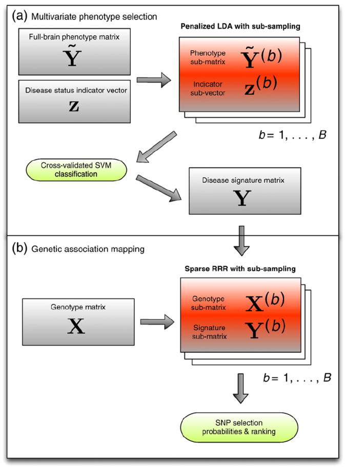
Flowchart illustrating the entire procedure followed for this application. In step (a) the phenotypes, consisting of the most discriminative voxels, are defined using penalized LDA and in step (b) these are used within the sRRR model in search of imaging genetic associations.

3. Results

3.1. Disease signatures from longitudinal imaging data

We report on the three classification experiments separately: AD vs CN, P-MCI vs CN, and P-MCI vs S-MCI. For each experiment, the selection of discriminative voxels was carried out according to the classification procedure described in the Penalized linear discriminant analysis for voxel filtering section combined with the model selection procedure, described in the Stability selection section. We fix the regularization parameter to estimate the direction vector with a fixed number of non-zero elements, and estimate the frequency of selection of each voxel across B = 100 random sub-samples.

In order to determine a probability threshold for the final selection of voxels to be retained in the signature, we assess the discriminative power of the selected set of voxels for different probability thresholds. To do this we apply the SVM classifier with a Gaussian kernel. With this choice of classifier, there are three parameters to be optimized, which we collect in a parameter vector θ = {π, σ, C}: π controls the voxels selected in S during the feature selection stage with penalized LDA, whereas σ and C are the kernel width and the regularization parameter of the SVM classifier, respectively. The optimal parameter vector θ* = {π*, σ*, C*} was obtained by 10-fold cross validation of three performance measures: accuracy, sensitivity and specificity. These cross validated performance measures are all reported in Table 2. The accuracy index, representing the percentage of correctly classified individuals, is between 82.1% (for the P-MCI vs S-MCI group) and 90.3% (for the AD vs CN group) and requires less than 13k voxels in all cases. In Fig. 2 we illustrate the two-dimensional patterns of the imaging signatures, extracted using multidimensional scaling. Notably, a non-linear classifier, as the one used here seems more suitable for separating the different classes of individuals.

Table 2.

Number of selected voxels (vox) and 10-fold cross validated performance measures in % – accuracy (acc), sensitivity (sen) and specificity (spe) – using a SVM classifier with Gaussian kernel.

Groups	vox	acc	sen	spe
AD vs CN	11,394	90.3	87.5	92.1
P-MCI vs CN	12,664	86.9	81.2	90.9
P-MCI vs S-MCI	10,593	82.1	81.5	82.9

Fig. 2.

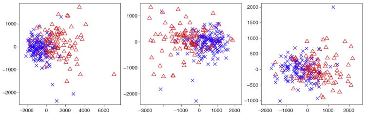
Two-dimensional representation of all the subjects obtained by multi-dimensional scaling of the imaging signatures identified by sparse LDA: AD versus CN (left), P-MCI versus CN (middle) and P-MCI versus S-MCI (right). The blue crosses refer to the ‘healthy’ class, that is the CN individuals in the left and middle plots and the S-MCI individuals in the right plot. The red triangles refer to ‘diseased’ class, that is AD patients in the left and the P-MCI patients in the middle and right plots.

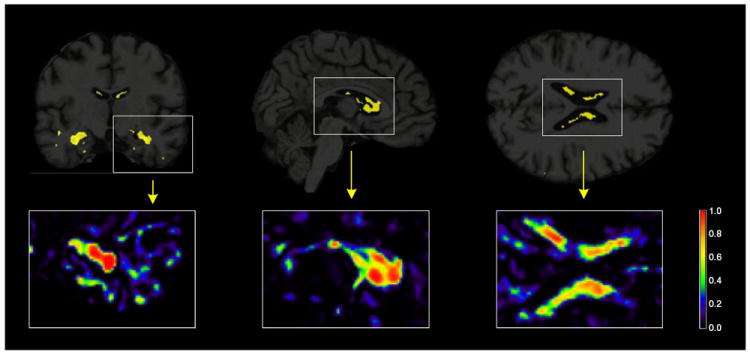
Figs. 3-5 show MRI scans with voxels in Ŝ (π*) in yellow, for all comparisons in Table 2. As an illustration, the insets show the whole range of selection probabilities P̂_j for all the voxels, without any thresholding. The most discriminative voxels are mostly clustered in the hippocampus and lateral ventricles. Parts of the temporal lobe, amygdala and caudate nucleus are also amongst the other key structures contributing to the selected voxels in the AD vs CN and P-MCI vs CN comparisons. A more widespread pattern of selected voxels is obtained from the P-MCI versus S-MCI comparison, where again the main selected structures are the lateral ventricles and the hippocampus but several parts of the brain lobes also contribute a relatively large amount of voxels. The distribution of the entire sets of selected voxels in the brain are given in the Supplementary Tables 1, 3 and 5 for the AD vs CN, P-MCI vs CN and P-MCI vs S-MCI comparisons, respectively. These patterns of widespread atrophy are in agreement with previous findings from both neuropathological studies as well as baseline and longitudinal morphological studies (Braak et al., 1999; Cuingnet et al., 2011; Hua et al., 2009; Leow et al., 2009; Misra et al., 2009). Being highly discriminative, the selected voxels provide a quantitative characterization of the disease that can be used as a phenotype in gene mapping studies.

Fig. 3.

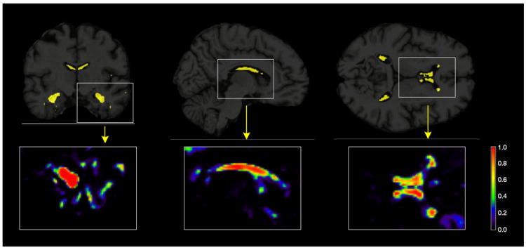
Brain images showing the results from the penalized LDA analysis of the AD versus CN comparison. The selected voxels are illustrated in yellow for the 3 plane of views of the brain (coronal, sagittal and axial from left to right). Illustrations of the actual selection probabilities are shown in color scale in the insets below.

Fig. 5.

Brain images showing the results from the penalized LDA analysis of the P-MCI versus S-MCI comparison. The selected voxels are illustrated in yellow for the 3 plane of views of the brain (coronal, sagittal and axial from left to right). Illustrations of the actual selection probabilities are shown in color scale in the insets below.

In order to assess the statistical significance of the accuracy of the estimated signatures, reported in Table 2, we carried out non-parametric inference using permutation testing. Holding the optimal θ* constant, we randomly permuted the individual class labels, z, and repeated this procedure M times. For each m, with m = 1,…, M, we applied the SVM classifier to the data containing the selected voxels and the permuted class indicator vector and produced the corresponding 10-fold cross-validated accuracy measure. This procedure approximates the sampling distribution of the accuracy index under the null hypothesis of no association between the voxel intensities in Ŝ(π*) and the class indicators, and an empirical p-value can be easily computed. Using M = 1000 permuted data sets, the accuracy results in Table 2 were all found to be highly significant (p-values <0.001).

3.2. Genetic association results

We searched for genetic associations with the sets of discriminative voxels, selected from each comparison, as shown in Figs. 3-5, by conducting the three corresponding imaging genetics studies. We do so using the sRRR model, described in the Sparse reduced-rank regression section. By fixing the regularization parameter λ_b such that a fixed number of SNPs are included in the model, we examine a possible range of number of selected SNPs. Using stability selection, with the number of extracted sub-samples B = 500, we are able to rank the SNPs based on their importance in the model. For each study, we report on the top 10 SNPs with maximum selection probability (across the path of the regularization parameter) greater than or equal to 0.5. Note that, in each case, in order to move to the following rank we fix the selection probability threshold to be equal to 0.5 and regress out the effect of the variables exceeding this threshold as shown in Eq. (5). As mentioned in the Sparse reduced-rank regression section, different ranks of the model are expected to capture different genetic effects on the disease phenotypes. Some remarks on several top scoring SNPs, corresponding to genes that are implicated in AD or that show potential susceptibility, are given below.

AD versus CN analysis

The top ten SNPs with selection probability exceeding 0.5, from the first three ranks of the sRRR model, are summarized in Table 3 and a complete list of the SNPs with selection probability ≥0.5 is given in Supplementary Table 2. The corresponding selection probabilities for all the SNPs are illustrated in Fig. 6. Here, the APOE-ε4 variant of the APOE gene scores top of the list with a selection probability approximately equal to 1. This means that the allele was chosen as an important variable in almost all of the 500 sub-samples. This variant of the APOE gene has long been known as the main high risk factor for AD, and has been replicated in numerous studies, including case control studies as well as studies involving biomarkers extracted from brain images (Barabash et al., 2009; Filippini et al., 2009; Zuo et al., 2006). As reviewed by Braskie et al. (2011), the APOE gene has been associated with a number of brain regions, including hippocampus, parahippocampal gyrus, amygdala and temporal lobe, which also constitute the regions within which the majority of our selected voxels lie. While the ε4 variant is associated with an increased risk of developing the disease, the ε2 variant is considered to be protective and is associated with a lower disease risk, whereas the ε3 variant is supposed to have a neutral effect on disease risk. Accordingly, the variants of the APOE gene are expected to be involved in the aggregation and clearance of the amyloid β protein, which provides a possible explanation for its key role in AD (Kim et al., 2009). The APOE gene also shows regulation and alternative splicing in the temporal lobe of AD patients compared to controls (Twine et al., 2011).

Table 3.

The top ten SNPs with maximum selection probabilities ≥0.5 (ranked according to their selection probabilities) for ranks 1, 2 and 3 of the AC versus CN sRRR analysis. For each marker also provided are: the corresponding gene annotation, where applicable, the chromosome, the MAF, the HWE p-value and the selection probability.

AD vs CN
SNP		Gene	Chr	MAF	HWE	P̂xj
Rank 1	APOE-ε4	APOE	19	0.276	0.083	0.996
	rs2075650	TOMM40	19	0.252	0.868	0.944
	rs3815501	BZW1	2	0.154	0.470	0.758
	rs11132507		4	0.284	0.643	0.705
	rs11132508		4	0.284	0.643	0.705
	rs1681052	LOC647946	18	0.077	0.647	0.681
	rs7761213		6	0.303	0.458	0.675
	rs17345545		1	0.266	0.422	0.647
	rs13340334	PDZD2	5	0.112	0.336	0.611
	rs17103124		14	0.152	0.623	0.605
Rank 2	rs9263844		6	0.161	1.000	0.772
	rs9263846		6	0.161	1.000	0.772
	rs7999394	MTRF1	13	0.408	0.027	0.746
	rs3794328	MTRF1	13	0.408	0.027	0.746
	rs11590365		1	0.114	0.547	0.621
	rs11204949		1	0.114	0.547	0.621
	rs11204971		1	0.114	0.547	0.621
	rs12405278	FLG	1	0.114	0.547	0.621
	rs215340		12	0.248	1.000	0.593
	rs7603289		2	0.345	0.330	0.585
Rank 3	rs727432	ADCY2	5	0.282	0.877	0.709
	rs11783329		8	0.398	0.435	0.589
	rs7114756	MAML2	11	0.161	0.059	0.581
	rs17309585		8	0.406	1.000	0.526
	rs10491327		5	0.183	0.143	0.520
	rs12534148	PDE1C	7	0.270	0.153	0.506

Fig. 6.

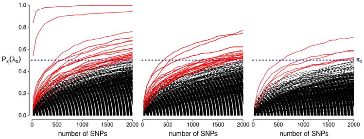
Stability selection probabilities for the AD versus CN analysis for ranks 1, 2 and 3 (from left to right). Each line corresponds to each SNP in the analysis and represents its selection probability (y-axis) while varying the number of SNPs to be retained in the model (x-axis). Lines corresponding to SNPs with maximum selection probabilities greater than or equal to the threshold π_x = 0.5 are illustrated in red. This probability threshold is illustrated by a horizontal blue line at P_xj(λ_b) = 0.5.

The SNP rs2075650, which belongs to the TOMM40 gene, also scores very highly with a selection probability of 0.94. The TOMM40 gene is located in close proximity to the APOE gene and has also been linked to AD in some more recent studies. For example, an association between the same SNP rs2075650 with hippocampus and amygdala was reported by Shen et al. (2010), who performed a MULM genome-wide association analysis with 142 phenotypes extracted from baseline MRI scans, and observed on 733 individuals from the ADNI study. Other studies reporting association with this SNP and AD include the works by Potkin et al. (2009) and Harold et al. (2009). In a phylogenetic analysis, Roses et al. (2009) have shown, from two independent cohorts, that the rs10524523 marker, also located in the TOMM40 gene, is associated with increased disease risk. They also highlighted some possible interactions with the APOE gene, and in particular with the APOE-ε3 variant which, as mentioned earlier, is supposed to have a neutral effect in AD (Grossman et al., 2010). This gene codes for the translocase of the outer mitochondrial membrane through which proteins are imported into mitochondria. Mitochondrial dysfunction is also known to contribute to neurodegeneration leading to the onset of AD (Wang et al., 2009).

The BZW1 gene, coding for basic leucine zipper and W2 domains 1, scores third in the list, with selection probability of 0.76. No prior association between BZW1 and AD has been previously reported. However, the gene was listed amongst the differentially expressed genes (with a p-value 0.026), from a microarray analysis on a mouse model related to a neurodegenerative disease called amyotrophic lateral sclerosis (Brockington et al., 2010). It has also shown differential expression in the central nervous system of mice during infection with mouse-adapted scrapie agents (Booth et al., 2004).

The PDZD2 gene, coding for the protein containing PDZ domain 2, has been selected with a probability of 0.61. This gene is known to interact with CST3 (Lindahl et al., 1992), which codes for cystatin 3 protein and has been previously reported as a susceptibility risk factor in AD. However, the results regarding the association of the CST3 gene with AD are conflicting; while several studies have reported an association with the CST3 gene (e.g. (Cathcart et al., 2005)), others failed to do so (e.g. (Monastero et al., 2005)). Three SNPs in the YES1 gene also score highly in the rank 1 results with selection probabilities around 0.5 (see Supplementary Table 2). A possible link between this gene and AD has been suggested (Stephanie, 2008).

The second rank analysis selects with probability 0.75 two SNPs in MTRF1, which is a gene encoding mitochondrial translational release factor 1. There is no evidence associating this gene with AD in the literature, however its function may suggest a possible contribution to mitochondrial dysfunction related to the disease. In the third rank, the model selects the ADCY2 gene, coding for adenylate cyclase 2, ranked top with a selection probability of 0.71. In a gene expression study in mice, Tsolakidou et al. (2010) revealed new pathways related to stress response, expressed in the periventricular nucleus of the hypothalamus, involving the ADCY2 gene together with the well-established early onset AD risk factor, the APP gene.

To examine the expression of the selected genes in the brain, we used the Allen Human Brain atlas.⁵ This atlas provides the tools to visualize histology and gene expression data from microarray and in situ hybridization studies on the brain. We were able to confirm that the reported genes are expressed in areas where our selected voxels lie such as in the hippocampus region, the inferior and middle temporal gyrus, the occipitotemporal gyrus, the parahippocampal gyrus, the fusiform gyrus, the amygdala and the caudate nucleus.

P-MCI versus CN analysis

The top ten SNPs with selection probability exceeding 0.5 from the P-MCI versus CN experiment are given in Table 4 and a complete list of the SNPs with selection probability ≥0.5 is given in Supplementary Table 4. The corresponding selection probabilities for all the SNPs are illustrated in Fig. 7. The APOE-ε4 variant again scores top of the list with a selection probability approximately equal to one. The same TOMM40 SNP that scored second in the AD vs CN rank 1 comparison, also scored among the top SNPs in the P-MCI vs CN comparison with a selection probability of 0.59. MYO3B, coding for the myosin III B protein, is another gene amongst the top scoring genes in the rank 1 analysis. This gene is known to be expressed in the retina and is possibly associated with visual disorders (Brown and Bridgman, 2004). RBFOX1 coding for the ataxin-2 binding protein 1 (also known as A2BP1) also scored highly with probability 0.57. This gene has been associated to autism, bipolar disorder, mental retardation and epilepsy (Baum et al., 2008; Bhalla et al., 2004; Hamshere et al., 2009; Martin et al., 2007).

Table 4.

The top ten SNPs with maximum selection probabilities ≥0.5 (ranked according to their selection probabilities) for ranks 1, 2 and 3 of the P-MCI versus CN sRRR analysis. For each marker also provided are: the corresponding gene annotation, where applicable, the chromosome, the MAF, the HWE p-value and the selection probability.

P-MCI vs CN
SNP		Gene	Chr	MAF	HWE	P̂xj
Rank 1	APOE-ε4	APOE	19	0s.271	0.083	0.982
	rs2883782	MYO3B	2	0.483	0.387	0.746
	rs2798062		9	0.256	0.105	0.712
	rs10934170		3	0.146	0.619	0.681
	rs17826780		4	0.102	0.318	0.665
	rs7843577		8	0.448	1.000	0.617
	rs2075650	TOMM40	19	0.246	0.180	0.589
	rs1405443		7	0.135	1.000	0.583
	rs758491	RBFOX1	16	0.352	1.000	0.566
	rs914166		21	0.150	0.624	0.548
Rank 2	rs13132552	SORBS2	4	0.348	1.000	0.792
	rs12633719		3	0.233	0.490	0.671
	rs11069874		13	0.158	0.242	0.661
	rs885339		13	0.158	0.242	0.661
	rs2381958		5	0.204	0.343	0.655
	rs10041184		5	0.217	0.146	0.639
	rs4265409		1	0.440	0.706	0.627
	rs7584948	ANTXR1	2	0.187	0.105	0.623
	rs501435	ODZ4	11	0.150	0.811	0.599
	rs1001684		5	0.265	0.874	0.595
Rank 3	rs705837	PRSS12	4	0.375	0.895	0.639
	rs11856999	MAP2K5	15	0.148	0.227	0.605
	rs7653663	MGLL	3	0.165	0.111	0.601
	rs12597064		16	0.240	1.000	0.570
	rs633398	NDST3	4	0.373	0.895	0.546
	rs631271	NDST3	4	0.371	1.000	0.544
	rs1529442	AQPEP	5	0.323	0.201	0.542
	rs6864491	AQPEP	5	0.450	0.802	0.534
	rs10445932	NRXN1	2	0.106	0.750	0.518
	rs885120	AQPEP	5	0.489	0.621	0.512

Fig. 7.

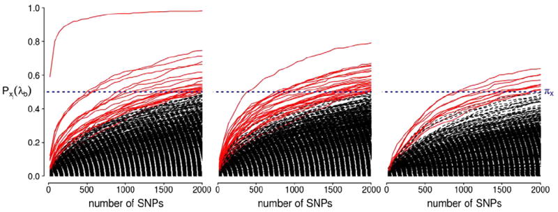
Stability selection probabilities for the P-MCI versus CN analysis for ranks 1, 2 and 3 (from left to right). Each line corresponds to each SNP in the analysis and represents its selection probability (y-axis) while varying the number of SNPs to be retained in the model (x-axis). Lines corresponding to SNPs with maximum selection probabilities greater than or equal to the threshold π_x = 0.5 are illustrated in red. This probability threshold is illustrated by a horizontal blue line at P_xj(λ_b) = 0.5.

Two SNPs of the COX7A2L gene, coding for the cytochrome c oxidase subunit VIIa polypeptide 2 like, are also amongst the top results of the rank 1 analysis, selected with probabilities around 0.53 (see Supplementary Table 4). This COX7A2L gene belongs in the ‘Alzheimer’s disease’ KEGG pathway⁶ (Kanehisa et al., 2010) and is involved in the mitochondrial dysfunction network. Recently, Lambert et al. (2010) performed a GWA gene set enrichment analysis using a large sample of AD patients and controls, and found the ‘Alzheimer’s disease’ KEGG pathway to be significantly over-represented in their sample, with a p-value 0.001, after false discovery correction. Within this pathway, 46 genes, including the COX72AL gene and other key AD risk factors, showed significant associations with the disease (uncorrected p-values ≤0.01) and thus were mostly involved in the over-representation of this pathway. Moreover, physical interactions between the key AD risk factor TOMM40 and the COX7A2L gene have been previously reported (McFarland et al., 2008).

The SORBS2 gene, coding for the sorbin and SH3 domain protein 2, scored top in the second rank of the analysis with a selection probability of 0.79. This gene is known to interact with the SYNJ1 gene, coding for the synaptojanin protein (Zucconi et al., 2001). The latter seems to be highly expressed in the brain and it has shown possible associations with a number of neurological diseases including schizophrenia and bipolar disorder (Stopkova et al., 2004a, 2004b), as well as Down’s syndrome (Chang and Min, 2009). It is also reported to interact with the BIN1 gene (Micheva et al., 1997), one of the top 10 susceptibility genes in AD, according to the Alzgene database as of July 2011.

The NRXN1 gene, coding for the neurexin 1 protein, is among the top results in rank 3 of the P-MCI vs CN analysis with a selection probability of 0.52. This gene was mentioned in Ravetti et al. (2010) who analyzed hippocampal gene expression data. In this study, using a sample consisting of subjects with different degrees of disease severity, from control to severe AD, the authors calculated the Jensen–Shannon divergence of each individual from the average control profile and from the average severe AD profile. They then computed the correlation coefficients between the gene expressions and the divergence measures, and reported the top 100 genes correlated with the control divergence, and the top 100 genes correlated with the severe AD divergence. The expression of NRXN1 was among these lists, showing a relatively high positive correlation (0.748) with the average severe AD profile, and a negative correlation (−0.706) with the average control profile. The NRXN1 has also been linked to schizophrenia and autistic spectrum disorder (Mühleisen et al., 2011; Reichelt et al., in press).

We examined the expressions of these genes in the brain using the Allen Brain Atlas. We found that these were expressed in the regions where the selected voxels mostly lie, including the hippocampus region, the inferior, middle and superior temporal gyrus, the occipitotemporal gyrus, the parahippocampal gyrus, the fusiform gyrus, the amygdala, the caudate nucleus and the insula.

P-MCI versus S-MCI analysis

In Table 5 we report the top ten SNPs with selection probabilities exceeding 0.5 for the P-MCI versus S-MCI experiment. A complete list of the SNPs with selection probability ≥0.5 is given in Supplementary Table 6. The corresponding selection probabilities for all the SNPs are illustrated in Fig. 8. The APOE-ε4 variant again scores top of the rank 1 results with high selection probability. The MGMT gene also scores highly. Using the Allen Brain Atlas, we confirmed that the MGMT gene is expressed in the brain regions where our selected voxels mostly lie, including the hippocampus, the amygdala and the temporal and frontal lobes. However, its association with AD is not clear. These results are associated with disease progression rather than development which is a possible reason for the limited validation through the current literature.

Table 5.

The top ten SNPs with maximum selection probabilities ≥0.5 (ranked according to their selection probabilities) for ranks 1, 2 and 3 of the P-MCI versus S-MCI sRRR analysis. For each marker also provided are: the corresponding gene annotation, where applicable, the chromosome, the MAF, the HWE p-value and the selection probability.

P-MCI vs S-MCI
SNP		Gene	Chr	MAF	HWE	P̂xj
Rank 1	APOE-ε4	APOE	19	0.346	0.300	0.903
	rs2038358		14	0.240	0.459	0.774
	rs2615945		11	0.405	0.889	0.685
	rs2602629		2	0.498	0.005	0.683
	rs9633774		10	0.423	0.217	0.653
	rs12356435		10	0.312	0.876	0.641
	rs11256463		10	0.405	0.328	0.623
	rs7068256	MGMT	10	0.240	0.063	0.607
	rs8014021		14	0.158	0.801	0.599
	rs965566		5	0.319	0.644	0.588
Rank 2	rs12420917		11	0.401	0.576	0.573
Rank 3	rs10751709		12	0.292	0.418	0.754
	rs2703862		8	0.104	0.067	0.617
	rs2507717		8	0.106	0.079	0.597
	rs9295895		6	0.247	0.366	0.581
	rs10082970		12	0.215	0.432	0.548
	rs10503991		8	0.111	0.158	0.512
	rs6468370		8	0.111	0.158	0.512

Fig. 8.

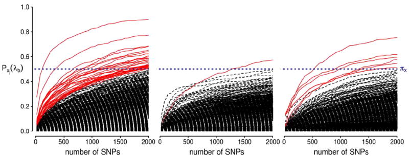
Stability selection probabilities for the P-MCI versus S-MCI analysis for ranks 1, 2 and 3 (from left to right). Each line corresponds to each SNP in the analysis and represents its selection probability (y-axis) while varying the number of SNPs to be retained in the model (x-axis). Lines corresponding to SNPs with maximum selection probabilities greater than or equal to the threshold π_x = 0.5 are illustrated in red. This probability threshold is illustrated by a horizontal blue line at P_xj(λ_b) = 0.5.

4. Discussion

AD is a highly prevalent disease with an estimate of 5.4 million patients, in the US alone (Alzheimer’s Association, 2011). As the risk for developing the disease increases with age, and due to the aging population, numbers are expected to increase dramatically over the next few decades, making Alzheimer’s one of the greatest concerns to society. Elucidating the genetic etiology of the disease holds great promise for uncovering its pathogenesis and thus contributing to an earlier diagnosis and treatment of the disorder. Much effort has been spent on identifying such genetic risk factors, but only a few markers have been detected and successfully replicated so far, mostly due to the lack of statistical power of existing case–control studies, which requires very large cohorts. The genetic variants discovered through these efforts are believed to account for only a small proportion of the total heritability.

Over the last few years, imaging genetics studies in AD and other neurodegenerative disorders have become popular as brain phenotypes extracted using neuroimaging techniques may constitute superior indicators of gene effects, as compared to categorical disease phenotypes, and are expected to ultimately yield higher statistical power. Although mass-univariate linear modeling is the commonly used approach, it suffers from a number of shortcomings, most notably due to its inability to detect small effects from multiple SNPs, or joint effects on multiple phenotypes, and the hypothesis testing framework involves a serious multiple testing problem. In this work we took a predictive modeling and variable selection approach, and examined the joint effects of multiple genetic markers to multiple imaging phenotypes in three genome-wide association studies with the objective to discover risk factors responsible for the progression of the disease.

A critical issue in the design of imaging genetics studies involves the definition and extraction of an appropriate multivariate disease phenotype. For our studies, we took voxel-wise Jacobian determinants, each one representing the longitudinal change observed between baseline and 24 month follow up images. Since AD is a progressive disorder with patterns of widespread brain atrophy that develop over time, longitudinal changes observed in MRI scans provide sensitive biomarkers reflecting disease development and progression. A separate issue concerns the selection of the specific voxels to be used in the study, and whether or not to take summary measures instead of individual voxels, in an attempt to reduce the dimensionality of the phenotype at the cost of losing some information. For instance, in cases when an anatomical atlas is available, it is common to average across all voxels within each ROI, thus drastically reducing the number of measurements that define the phenotype. In this paper we take an alternative approach and reduce the number of noise voxels by first detecting a localized signature of the disease consisting of as fewer voxels as possible. Our initial feature selection step was intended to reduce the dimensionality while also detecting regions that are subjected to change over time in a data-driven fashion, without any prior knowledge or subjective assumptions. Similar arguments have been made in other studies, for example by Hua et al. (2009) and Chen et al. (2010) who observed increased power in detecting AD-related changes, when using data-driven ROIs estimated from training samples, compared to using anatomically defined ROIs.

Voxel selection was achieved using a penalized LDA procedure which enabled the extraction of subsets of voxels that are highly discriminative of the two groups of individuals considered in each comparison. Alternative variable selection approaches such as penalized logistic regression or even simple univariate t-tests could have also been used for this purpose. In the derivation of the penalized LDA algorithm, we estimate the within-group scatter matrix to be diagonal, which is commonly done for problems such as ours in which the data points lie in extremely high dimensional spaces. Although the resulting approach then becomes more similar to a univariate one, the penalized LDA formulation is attractive for a number of reasons. Firstly, one can find better estimates of the within-group scatter matrix and use that for the derivation of the algorithm. Second, different penalties can be easily adapted in the penalized LDA formulation that better exploit the structural patterns observed in the brain images.

The voxels selected by penalized LDA, in each one of the three comparisons, mostly formed connected regions in the hippocampus and lateral ventricles, reflecting hippocampal atrophy and ventricular enlargement. These findings are fully consistent with patterns of AD atrophy demonstrated in previous neuropathological and morphological studies (Braak et al., 1999; Cuingnet et al., 2011; Leow et al., 2009; Misra et al., 2009, for example). The accuracy of the selected sets of voxels was assessed using a SVM classifier with Gaussian kernel. The classification performance reported was comparable to findings documented in the literature. For instance, for the AD versus CN comparison, typical classification accuracy has been reported to vary from 85% to 95% (Batmanghelich et al., 2009; Fan et al., 2008a; Klöppel et al., 2008; Vemuri et al., 2008), whereas for the P-MCI versus CN group comparison the accuracy varies between 70% and 81.8% (Batmanghelich et al., 2009; Fan et al., 2008a) and for the P-MCI versus S-MCI between 70% and 81.5% (Misra et al., 2009). Our results compare favorably to a recent meta-analysis (Cuingnet et al., 2011) of classification methods on a similar subset of baseline MRI images from the ADNI cohort. While our results for AD versus CN classification were comparable to the best results reported in this study, we achieved significantly better results for P-MCI versus CN classification and for the clinically most interesting discrimination of progressive from stable MCI subjects (P-MCI vs S-MCI).

Although we have found that the selected voxels all cluster in compact regions of the brain, fewer isolated voxels can still found to be scattered in other disconnected regions, whose association to disease status may be less clear. The penalized LDA approach could be further extended to introduce some form of spatial regularization. For example, the l_{2, 1} group penalty combined with the l₁ penalty (Friedman et al., 2010) could be used to select subsets of voxels within ROIs defined according to an anatomical atlas. This extra information can further eliminate the noisy variables from our sets of selected voxels, by encouraging voxels within a ROI to stay grouped together during the voxel selection process.

Gene association mapping was carried out by searching for genetic variants that are highly predictive of the imaging signatures detected in the first analysis stage. This was accomplished by the means of sparse reduced-rank regression, a penalized regression model that encourages the identification of joint effects of multiple genetic markers onto multiple phenotypes. Due to the strong structural patterns observed in brain images, true genetic associations are expected to show homogeneous patters in neighboring voxels, forming localized regions. Hence, combining the voxel filtering technique with the multivariate imaging genetics analysis, our experiments greatly benefit from the enhanced signals of association present at the phenotypes, being highly discriminative for the disease, as well as from the structural homogeneity, by taking into account the simultaneous genetic effects on nearby voxels. At the cost of additional model complexity, sRRR can be extended in a straightforward manner to induce sparsity in the phenotypic level, and enable the identification of even smaller brain regions that manifest a heritable component (Vounou et al., 2010). We opted not to follow this approach here, to keep the model as simple as possible, and avoid introducing additional regularization parameters. Moreover, the initial discriminative analysis allowed us to detect specific disease-related brain regions to use as phenotypes.

The difficult model selection problem, and in particular the selection and ranking of SNPs, was approached using a data re-sampling technique. Rather than using some cross-validated measures of predictive performance to guide the variable selection process, our data re-sampling scheme puts more emphasis on estimating the relative importance of each SNP by mimicking the process of extracting small random samples from the underlying population, and fitting a penalized model on each sample. This procedure provides a mechanism to rank SNPs based on the frequency in which they have been selected across all the sub-samples. The selection probability of a SNP then represents a robust metric for ranking purposes that more accurately reflect the relative importance that each marker plays in predicting the phenotype. The sRRR model also assumes that the underlying contributions from multiple SNPs will be captured by different hidden factors, or ranks. For each factor, the penalization term in the model forces the selection of only a few important SNPs contributing to it.

An important lesson learned from the extensive simulation experiments presented in Vounou et al. (2010) was that, when the signal to noise ratio is very small, the first rank may capture spurious associations with the disease, and therefore more than one rank is needed to be extracted to detect all potential and meaningful associations. An important issue is then how many latent factors or ranks to extract, and how to remove the genetic effects found in previous ranks before moving on to the next ones. In the studies presented here, we thresholded the SNP selection probabilities associated to a given latent factor so that the effects of all SNPs having a selection probability at least as high as 0.5 were removed prior to extracting the consecutive factor. A threshold of 0.5 means that any SNP selected in at least half of all the sub-samples are deemed to be important for that factor, and their effect will be removed before re-fitting the model and extracting the next rank. Although a higher and therefore stricter threshold may be used, we opted for a less conservative one, and examined up to three ranks.

All three GWA studies presented here identified the APOE-ε4 variant of the APOE gene as the most important marker to explain the longitudinal phenotypes. In all experiments this SNP ranked first with a selection probability greater than 0.9. This consistent result reflects both the importance of the APOE-ε4 variant in disease development but also its key involvement in the progression from MCI to AD. Together with APOE-ε4, the rs2075650 marker from TOMM40 gene, another key risk factor of AD, was also selected amongst the top results of the AD versus CN and P-MCI versus CN analysis. Remarkably this marker did not rank high in the P-MCI versus S-MCI analysis. Among our other reported results, the COX7A2L and NRXN1 genes from the P-MCI versus CN analysis also seem particularly interesting. The first is known to contribute in the mitochondrial dysfunction network of a KEEG pathway related to AD, while the latter has shown to be differentially expressed in AD. The other factors identified from our analyses were novel, in that they haven’t been reported in the literature before in association with AD. Among these we highlighted a number of genes, including BZW1, PDZD2, YES1, ADCY2, RBFOX1 and SORBS2. Some of these have been previously associated with other neurological disorders, whereas others had possible links to AD through interactions with other susceptibility markers. Further biological investigations of the reported results are necessary in order to validate their involvement in the disease.

5. Conclusions

In this work, we made a number of contributions, summarized as follows: (a) we extended the sRRR model and proposed a sub-sampling strategy for the selection and ranking of SNPs associated to a multivariate phenotype; (b) we presented a framework for quantifying the loss of statistical power that is expected when averaging across voxels, rather than using the voxels directly, thus formalizing the intuition that a voxel-wise approach is to be preferred, provided that the majority of voxels being considered as phenotypes are highly representative of the disease; (c) to detect reliable signatures of the disease, we carried out feature selection using penalized discriminative analysis, with a classification performance comparable with state-of-art results; and (d) we applied the sRRR model for the detection of genetic biomarkers in Alzheimer’s disease using data from the ADNI, carried out three genome-wide association studies, and reported on genetic associations detected by the sRRR model in each study. Our results confirmed the important role of known risk-bearing genes such as APOE-ε4 and TOMM40, but also highlighting other potential candidates that warrant further investigation.

Motivated by the promising results reported here, disease signatures derived from multiple imaging modalities are currently being considered. A number of recent studies indicate that superior discriminative performance between different clinical groups can be achieved by combining different imaging phenotypes. In particular, Kohannim et al. (2010) combined multiple biomarkers, including MRI and FDG-PET measures as well as CSF and other biomarkers for disease status classification using SVM classifiers and reported an increase in power to predict future decline. In another recent study, Li et al. (2012) obtained improved classification performance when considering a combination of features representing both static and longitudinal measures, as well as summary measures from constructed brain networks. Using a kernel approach, Zhang et al. (2011) also integrated information from baseline MRI, FDG-PET and CSF biomarkers, which were then used for classification using SVMs. According to their findings, a remarkable improvement is observed when fusing multiple modalities. Evidence from other similar studies suggest that more complex phenotypes derived from combining cross-sectional and longitudinal changes, from multiple modalities, and possibly taking into account connectivity networks, may carry higher discriminative power, and therefore provide higher signal to detect associations with the disease (Fan et al., 2008b; Vemuri et al., 2009; Walhovd et al., 2010, for instance). Finally, the sRRR model can be easily extended to use prior information on gene function by grouping genes and associated SNPs into gene sets or pathways (Silver and Montana, in press). By jointly considering the effects of multiple SNPs or genes within a biological pathway, significant associations might be identified that would otherwise be missed when considering markers individually.

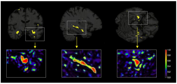
Fig. 4.

Brain images showing the results from the penalized LDA analysis of the P-MCI versus CN comparison. The selected voxels are illustrated in yellow for the 3 plane of views of the brain (coronal, sagittal and axial from left to right). Illustrations of the actual selection probabilities are shown in color scale in the insets below.

Appendix A

ROI averages and potential loss of power

Extracting ROI summaries, such as the average value across all voxels within a ROI (e.g. an anatomical region), is a common procedure in imaging genetics as an attempt to reduce dimensionality. In this appendix we propose a simple mathematical framework demonstrating that such an approach can potentially yield a smaller SNR, compared to the alternative approach that uses all voxels directly, without any summarization. We consider the case where all voxels have been grouped into K disjoint anatomical ROIs, and a single average is taken to represent each ROI. We show that a notable reduction in signal is expected when only a small subregion of a ROI is truly dependent on the genetic factors. When this is the case, taking averages will decrease the statistical power to detect the true genetic associations.

We start by introducing some notation. We assume that, within a ROI k, there are exactly g_k voxels, and we refer to this group of voxels within ROI k as f_k, for k = 1,…,K. Furthermore, we denote the reduced n×g_k matrix corresponding to ROI k observed on all n subjects by Ỹ_fk, and take ỹ_fkj, to be the vector containing the n observations for the jth voxel in ROI k. We then construct the n×K matrix, $\overline{\stackrel{\sim }{\mathbf{Y}}}$, such that its kth column, ${\overline{\stackrel{\sim }{\mathbf{y}}}}_k$, represents the average of the voxels across the kth ROI. We aim to quantify the SNR of both Ỹ and $\overline{\stackrel{\sim }{\mathbf{Y}}}$, to study whether taking averages across ROIs decreases the SNR. This is achieved by assuming an additive genetic model, according to which we pose that

$$\stackrel{\sim }{\mathbf{Y}}=\mathbf{Xb}a+\mathbf{E}$$

where the 1×g coefficient vector a has non-zero entries only for the voxels that are assumed to be involved in the disease. The p×1 vector b contains the genetic coefficients, which can be zero for those genetic marker that do not contribute to explain the variability in the response. The n×g matrix E corresponds to the model residuals.

Suppose that, among all the available ROIs, only d<K depend on genetic effects, whereas the remaining ones do not. For notational simplicity, we arrange the K ROIs f_k in the following order: the first d ROIs, that is those indexed k = 1,…,d, are the affected ones, and the remaining ones, indexed by k = d + 1,…,K are the unaffected ones. Furthermore, we assume that the signal of genetic association is localized in a percentage 0< t_k ≤ 1 of the overall number of voxels contained in a ROI, for k = 1,…,d, constituting the affected voxels. We call these t_kg_k voxels the signal voxels, and we also assume that these are ordered to appear first in each group f_k. Fig. 9 provides a schematic illustration of a set of K ROIs (in this case, a brain atlas): a selected ROI k (colored in dark yellow), could either contain all signal voxels, all having the same signal intensity (all denoted in black), or only contain a varying number of signal voxels, each one having varying signal intensities (denoted by grades of black).

Fig. 9.

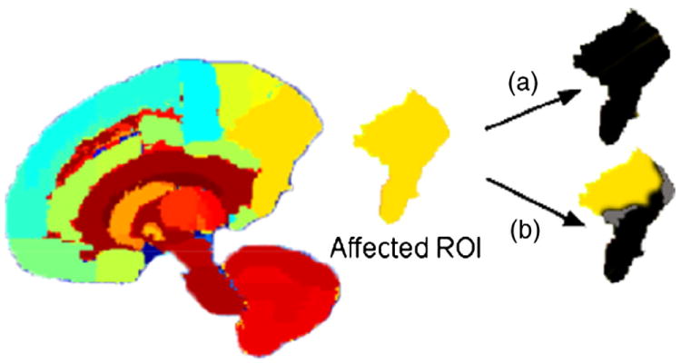
Sagittal view of a color-coded atlas of the brain. A ROI k (in dark yellow) has been picked to illustrate two possible scenarios: (a) all the voxels within the ROI are signal voxels, (b) the signal is gathered in a smaller subregion of the ROI. The signal intensity is represented by shades of black.

According to this model, the jth voxel in ROI f_k is then modeled such that

$${\stackrel{\sim }{\mathbf{y}}}_{f_{\mathit{kj}}}=\mathbf{Xb}{a}_{f_{\mathit{kj}}}+e_{f_{\mathit{kj}}}$$

for k = 1,…,d and j = 1,…, t_kg_k, or otherwise is e_fkj, where a_fkj is the coefficient corresponding to the jth voxel of ROI k. Extracting ROI averages then amounts to estimating the kth column of the n×K matrix $\overline{\stackrel{\sim }{\mathbf{Y}}}$ by

$${\overline{\stackrel{\sim }{\mathbf{y}}}}_k=\{\begin{array}{ll}\frac{1}{g_k}\mathbf{Xb}\sum _{j=1}^{t_k{g}_k}{a}_{f_{\mathit{kj}}}+\frac{1}{g_k}\sum _{j=1}^{g_k}{e}_{f_{\mathit{kj}}}& \mathrm{for}k=1,\dots ,d\\ \frac{1}{g_k}\sum _{j=1}^{g_k}{e}_{f_{\mathit{kj}}}& \mathrm{otherwise}.\end{array}$$

Having introduced these quantities, we can define the SNR for the jth voxel in ROI k as

$${\mathrm{SNR}}_{\stackrel{\sim }{\mathbf{y}}}{f}_{\mathit{kj}}=\frac{a_{f_{\mathit{kj}}}^2{\mathbf{b}}^{\prime }\mathrm{Var}(\mathbf{X})\mathbf{b}}{\mathrm{Var}\left(e_{f_{k_j}}\right)}$$

for k = 1,…,d and j = 1,…, t_kg_k, or otherwise this is 0. Analogously, the average SNR for the entire set of voxels, denoted by SNR_Ỹ, can be found to be

$${\mathrm{SNR}}_{\stackrel{\sim }{\mathbf{Y}}}=\frac{1}{g}{\mathbf{b}}^{\prime }\mathrm{Var}(\mathbf{X})\mathbf{b}\sum _{k=1}^K\sum _{j=1}^{t_k{g}_k}\frac{a_{f_{k_j}}^2}{\mathrm{Var}\left(e_{f_{k_j}}\right)}.$$ (6)

This expression may be simplified further by imposing that the coefficients in a are such that their weighted sum of squares, with weights given by the inverse of the variances, is constrained to be 1, that is

$$\sum _{k=1}^K\sum _{j=1}^{t_k{g}_k}\frac{a_{f_{k_j}}^2}{\mathrm{Var}\left(e_{f_{k_j}}\right)}=1,$$

which means that Eq. (8) reduces to

$${\mathrm{SNR}}_{\stackrel{\sim }{\mathbf{Y}}}=\frac{1}{g}{\mathbf{b}}^{\prime }\mathrm{Var}(\mathbf{X})\mathbf{b}.$$ (7)

On the other hand, the SNR for the kth ROI average is given as

$${\mathrm{SNR}}_{\overline{\stackrel{\sim }{\mathbf{y}}}k}=\frac{{\left({\sum }_{j=1}^{t_k{g}_k}{a}_{f_{\mathit{kj}}}\right)}^2\mathbf{b}\prime \mathrm{Var}(\mathbf{X})\mathbf{b}}{\mathrm{Var}\left({\sum }_{j=1}^{g_k}{e}_{f_{k_j}}\right)}$$

for k = 1,…,d and 0 otherwise. From this, it can be seen that the average SNR for the entire set of ROI averages, denoted by $\mathrm{SNR}\overline{\stackrel{\sim }{\mathbf{Y}}}$, is given by

$${\mathrm{SNR}}_{\overline{\stackrel{\sim }{\mathbf{Y}}}}=\frac{1}{K}\sum _{k=1}^d\frac{{\left({\sum }_{j=1}^{t_k{g}_k}{a}_{f_{\mathit{kj}}}\right)}^2\mathbf{b}\prime \mathrm{Var}(\mathbf{X})\mathbf{b}}{\mathrm{Var}\left({\sum }_{j=1}^{g_k}{e}_{f_{k_j}}\right)}.$$ (8)

Taking the ratio between Eqs. (7) and (8), we obtain that

$$\frac{{\mathrm{SNR}}_{\overline{\stackrel{\sim }{\mathbf{Y}}}}}{{\mathrm{SNR}}_{\stackrel{\sim }{\mathbf{Y}}}}=Q$$

where Q is given by

$$Q=\frac{g}{K}\sum _{k=1}^d\frac{{\left({\sum }_{j=1}^{t_k{g}_k}{a}_{f_{\mathit{kj}}}\right)}^2}{\mathrm{Var}\left({\sum }_{j=1}^{g_k}{e}_{f_{k_j}}\right)}.$$ (9)

and the variance of the sum of residuals in ROI k is

$$\mathrm{Var}\left(\sum _{j=1}^{g_k}{e}_{f_{k_j}}\right)=\sum _{j=1}^{g_k}\mathrm{Var}\left(e_{f_{k_j}}\right)+2\sum _{s=1}^{g_k}\sum _{j>s}^{g_k}\mathrm{Cov}\left(e_{f_{\mathit{kj}}},e_{f_{\mathit{ks}}}\right).$$

A value of Q less than 1 means that extracting ROI averages leads to a lower SNR than the one present at the voxel level.

As the number of possible scenarios is too large, we consider here only one case consisting in a single affected ROI containing a proportion t_k of signal voxels, as in Fig. 9. Furthermore, we assume that all the non-zero coefficients in a are equal, thus a_fkj = m for j = 1,…,t_kg_k and 0 otherwise, with m satisfying

$$m^{-2}=\sum _{j=1}^{t_k{g}_k}{\mathrm{Var}}^{-1}\left(e_{f_{k_j}}\right)$$

so that a also satisfies the earlier assumption on the weighted sum of squares. Under these assumptions, Q simplifies to

$$Q=\frac{t_k^{2}g}{K{m}^{-2}\mathrm{Var}\left(\frac{1}{g_k}{\sum }_{j=1}^{g_k}{e}_{f_{k_j}}\right)}.$$

By assuming that everything but t_k is fixed in this expression, we can see that the maximum value of Q is reached when all of the voxels within the affected ROI are signal voxels, that is t_k = 1, and Q decreases towards its minimum value as t_k decreases. Moreover, Q decreases with increasing residual variances and increasing (positive) residual pairwise covariances between the voxels in the affected ROI, thus increasing the variance of the average $\frac{1}{g_k}{\sum }_{j=1}^{g_k}{e}_{f_{k_j}}$. In particular, $\mathrm{SNR}\overline{\stackrel{\sim }{\mathbf{Y}}}$ becomes smaller than SNR_Ỹ when the residual variance term satisfies

$$m^{-2}\mathrm{Var}\left(\frac{1}{g_k}\sum _{j=1}^k{e}_{f_{k_j}}\right)>\frac{t_k^{2}g}{K}.$$

According to this model, when the proportion of signal voxels is small or when the residual variances and covariances are large, we expect a potential power loss when using ROI averages as the phenotypes to be tested for genetic association.

The ratio Q is also directly proportional to the number of voxels in the data, g, meaning that Q is increasing/decreasing with increasing/decreasing g. When g is extremely large, as in whole brain studies, a large proportion of voxels are expected to only contribute to noise, in terms of the disease. In that case, the SNR of Ỹ would be very small, making the ratio Q more favorable towards $\overline{\stackrel{\sim }{\mathbf{Y}}}$. In this case, even though the signal is reduced by taking the average across the entire ROI, the SNR in the ROI phenotypes is larger than the one present in the voxel-wise phenotypes where a large amount of noise voxels are also considered. These observations suggest that removing all noise voxels, that is voxels that are not detectably associated with the disease, prior to the imaging genetics study may increase the statistical power.

Appendix B

ADNI

ADNI was launched in 2003 by the National Institute on Aging (NIA), the National Institute of Biomedical Imaging and Bioengineering (NIBIB), the Food and Drug Administration (FDA), private pharmaceutical companies and non-profit organizations, as a $60 million, 5-year public-private partnership. The primary goal of ADNI has been to test whether serial MRI, positron emission tomography (PET), other biological markers, and clinical and neuropsychological assessment can be combined to measure the progression of MCI and AD. Determination of sensitive and specific markers of very early AD progression is intended to aid researchers and clinicians to develop new treatments and monitor their effectiveness, as well as lessen the time and cost of clinical trials. The Principle Investigator of this initiative is Michael W. Weiner, M.D., VA Medical Center and University of California-San Francisco. ADNI is the result of efforts of many co-investigators from a broad range of academic institutions and private corporations, and subjects have been recruited from over 50 sites across the U.S. and Canada. The initial goal of ADNI was to recruit 800 adults, ages 55 to 90, to participate in the research – approximately 200 cognitively normal older individuals to be followed for 3 years, 400 people with MCI to be followed for 3 years, and 200 people with early AD to be followed for 2 years. For up-to-date information see www.adni-info.org.

References

- Alzheimer’s Association. Alzheimer’s disease facts and figures. Alzheimer’s Dement. 2011;7(2):208–244. doi: 10.1016/j.jalz.2011.02.004. [DOI] [PubMed] [Google Scholar]
- Atiya M, Hyman B, Albert M, Killiany R. Structural magnetic resonance imaging in established and prodromal Alzheimer disease: a review. Alzheimer Dis Assoc Disord. 2003;17(3):177–195. doi: 10.1097/00002093-200307000-00010. [DOI] [PubMed] [Google Scholar]
- Barabash A, Marcos A, Ancin I, Vazquez-Alvarez B, de Ugarte C, Gil P, Fernández C, Encinas M, López-Ibor J, Cabranes J. APOE, ACT and CHRNA7 genes in the conversion from amnestic mild cognitive impairment to Alzheimer’s disease. Neurobiol Aging. 2009;30(8):1254–1264. doi: 10.1016/j.neurobiolaging.2007.11.003. [DOI] [PubMed] [Google Scholar]
- Batmanghelich N, Taskar B, Davatzikos C. Information Processing in Medical Imaging. Springer; 2009. A general and unifying framework for feature construction, in image-based pattern classification; pp. 423–434. [DOI] [PubMed] [Google Scholar]
- Baum A, Akula N, Cabanero M, Cardona I, Corona W, Klemens B, Schulze T, Cichon S, Rietschel M, Nöthen M, et al. A genome-wide association study implicates diacylglycerol kinase eta (DGKH) and several other genes in the etiology of bipolar disorder. Mol Psychiatry. 2008;13(2):197–207. doi: 10.1038/sj.mp.4002012. [DOI] [PMC free article] [PubMed] [Google Scholar]
- Bertram L, McQueen M, Mullin K, Blacker D, Tanzi R. Systematic meta-analyses of Alzheimer disease genetic association studies: the AlzGene database. Nat Genet. 2007;39(1):17–23. doi: 10.1038/ng1934. [DOI] [PubMed] [Google Scholar]
- Bertram L, Lill C, Tanzi R. The genetics of Alzheimer disease: back to the future. Neuron. 2010;68(2):270–281. doi: 10.1016/j.neuron.2010.10.013. [DOI] [PubMed] [Google Scholar]
- Bhalla K, Phillips H, Crawford J, McKenzie O, Mulley J, Eyre H, Gardner A, Kremmidiotis G, Callen D. The de novo chromosome 16 translocations of two patients with abnormal phenotypes (mental retardation and epilepsy) disrupt the A2BP1 gene. J Hum Genet. 2004;49(6):308–311. doi: 10.1007/s10038-004-0145-4. [DOI] [PubMed] [Google Scholar]
- Booth S, Bowman C, Baumgartner R, Sorensen G, Robertson C, Coulthart M, Phillipson C, Somorjai R. Identification of central nervous system genes involved in the host response to the scrapie agent during preclinical and clinical infection. J Gen Virol. 2004;85:3459–3471. doi: 10.1099/vir.0.80110-0. [DOI] [PubMed] [Google Scholar]
- Boyes RG, Rueckert D, Aljabar P, Whitwell J, Schott JM, Hill DL, Fox NC. Cerebral atrophy measurements using Jacobian integration: comparison with the boundary shift integral. NeuroImage. 2006;32(1):159–169. doi: 10.1016/j.neuroimage.2006.02.052. [DOI] [PubMed] [Google Scholar]
- Braak H, Braak E. Neuropathological stageing of Alzheimer-related changes. Acta Neuropathol. 1991;82(4):239–259. doi: 10.1007/BF00308809. [DOI] [PubMed] [Google Scholar]
- Braak E, Griffing K, Arai K, Bohl J, Bratzke H, Braak H. Neuropathology of Alzheimer’s disease: what is new since A. Alzheimer? Eur Arch Psychiatry Clin Neurosci. 1999;249(9):14–22. doi: 10.1007/pl00014168. [DOI] [PubMed] [Google Scholar]
- Braskie M, Ringman J, Thompson P. Neuroimaging measures as endophenotypes in Alzheimer’s disease. Int J Alzheimers Dis. 2011;2011:490140. doi: 10.4061/2011/490140. [DOI] [PMC free article] [PubMed] [Google Scholar]
- Breiman L. Stacked regressions. Mach Learn. 1996;24(1):49–64. [Google Scholar]
- Breiman L, Friedman J. Predicting multivariate responses in multiple linear regression. J R Stat Soc B Methodol. 1997:3–54. [Google Scholar]
- Brockington A, Heath P, Holden H, Kasher P, Bender F, Claes F, Lambrechts D, Sendtner M, Carmeliet P, Shaw P. Downregulation of genes with a function in axon outgrowth and synapse formation in motor neurones of the VEGFδ/δ mouse model of amyotrophic lateral sclerosis. BMC Genomics. 2010;11(1):203. doi: 10.1186/1471-2164-11-203. [DOI] [PMC free article] [PubMed] [Google Scholar]
- Brown M, Bridgman P. Myosin function in nervous and sensory systems. J Neurobiol. 2004;58(1):118–130. doi: 10.1002/neu.10285. [DOI] [PubMed] [Google Scholar]
- Cathcart H, Huang R, Lanham I, Corder E, Poduslo S. Cystatin C as a risk factor for Alzheimer disease. Neurology. 2005;64(4):755–757. doi: 10.1212/01.WNL.0000151980.42337.44. [DOI] [PubMed] [Google Scholar]
- Chang K, Min K. Upregulation of three Drosophila homologs of human chromosome 21 genes alters synaptic function: implications for Down syndrome. Proc Natl Acad Sci. 2009;106(40):17117–17122. doi: 10.1073/pnas.0904397106. [DOI] [PMC free article] [PubMed] [Google Scholar]
- Chen K, Langbaum J, Fleisher A, Ayutyanont N, Reschke C, Lee W, Liu X, et al. Twelve-month metabolic declines in probable Alzheimer’s disease and amnestic mild cognitive impairment assessed using an empirically pre-defined statistical region-of-interest: findings from the Alzheimer’s Disease Neuroimaging Initiative. NeuroImage. 2010;51(2):654–664. doi: 10.1016/j.neuroimage.2010.02.064. [DOI] [PMC free article] [PubMed] [Google Scholar]
- Chiang M, Barysheva M, McMahon K, de Zubicaray G, Johnson K, Martin N, Toga A, Wright M, Thompson P. Biomedical Imaging: From Nano to Macro, 2011 IEEE International Symposium on. IEEE; 2011. Hierarchical clustering of the genetic connectivity matrix reveals the network topology of gene action on brain microstructure: an N = 531 twin study; pp. 832–835. [Google Scholar]
- Chun H, Keleş S. Sparse partial least squares regression for simultaneous dimension reduction and variable selection. J R Stat Soc B Stat Methodol. 2010;72(1):3–25. doi: 10.1111/j.1467-9868.2009.00723.x. [DOI] [PMC free article] [PubMed] [Google Scholar]
- Corder E, Saunders A, Strittmatter W, Schmechel D, Gaskell P, Small G, Roses A, Haines J, Pericak-Vance M. Gene dose of apolipoprotein E type 4 allele and the risk of Alzheimer’s disease in late onset families. Science. 1993;261(5123):921–923. doi: 10.1126/science.8346443. [DOI] [PubMed] [Google Scholar]
- Csernansky J, Wang L, Swank J, Miller J, Gado M, McKeel D, Miller M, Morris J. Preclinical detection of Alzheimer’s disease: hippocampal shape and volume predict dementia onset in the elderly. NeuroImage. 2005;25(3):783–792. doi: 10.1016/j.neuroimage.2004.12.036. [DOI] [PubMed] [Google Scholar]
- Cuingnet R, Gerardin E, Tessieras J, Auzias G, Lehéricy S, Habert M, Chupin M, Benali H, Colliot O. Automatic classification of patients with Alzheimer’s disease from structural MRI: A comparison of ten methods using the ADNI database. NeuroImage. 2011;56(2):766–781. doi: 10.1016/j.neuroimage.2010.06.013. [DOI] [PubMed] [Google Scholar]
- Davatzikos C, Xu F, An Y, Fan Y, Resnick S. Longitudinal progression of Alzheimer’s-like patterns of atrophy in normal older adults: the SPARE-AD index. Brain. 2009;132(8):2026–2035. doi: 10.1093/brain/awp091. [DOI] [PMC free article] [PubMed] [Google Scholar]
- DeKosky S, Marek K. Looking backward to move forward: early detection of neurodegenerative disorders. Science. 2003;302(5646):830–834. doi: 10.1126/science.1090349. [DOI] [PubMed] [Google Scholar]
- Duda R, Hart P, Stork D. Pattern Classification. Vol. 2. John Wiley & Sons; 2001. [Google Scholar]
- Eyler L, Prom-Wormley E, Fennema-Notestine C, Panizzon M, Neale M, Jernigan T, Fischl B, Franz C, Lyons M, Stevens A, et al. Genetic patterns of correlation among subcortical volumes in humans: results from a magnetic resonance imaging twin study. Hum Brain Mapp. 2011;32:641–653. doi: 10.1002/hbm.21054. [DOI] [PMC free article] [PubMed] [Google Scholar]
- Fan J, Li R. Variable selection via nonconcave penalized likelihood and its oracle properties. J Am Stat Assoc. 2001;96(456):1348–1360. [Google Scholar]
- Fan Y, Batmanghelich N, Clark CM, Davatzikos C. Spatial patterns of brain atrophy in MCI patients, identified via high-dimensional pattern classification, predict subsequent cognitive decline. NeuroImage. 2008a;39(4):1731–1743. doi: 10.1016/j.neuroimage.2007.10.031. [DOI] [PMC free article] [PubMed] [Google Scholar]
- Fan Y, Resnick S, Wu X, Davatzikos C. Structural and functional biomarkers of prodromal Alzheimer’s disease: a high-dimensional pattern classification study. NeuroImage. 2008b;41(2):277–285. doi: 10.1016/j.neuroimage.2008.02.043. [DOI] [PMC free article] [PubMed] [Google Scholar]
- Ferreira M, Purcell S. A multivariate test of association. Bioinformatics. 2009;25(1):132–133. doi: 10.1093/bioinformatics/btn563. [DOI] [PubMed] [Google Scholar]
- Filippini N, Rao A, Wetten S, Gibson RA, Borrie M, Guzman D, Kertesz A, Loy-English I, Williams J, Nichols T, Whitcher B, Matthews PM. Anatomically-distinct genetic associations of APOE ε4 allele load with regional cortical atrophy in Alzheimer’s disease. NeuroImage. 2009;44(3):724–728. doi: 10.1016/j.neuroimage.2008.10.003. [DOI] [PubMed] [Google Scholar]
- Fisher R, et al. The use of multiple measurements in taxonomic problems. Ann Eugenics. 1936;7:179–188. [Google Scholar]
- Folstein MF, Folstein SE, McHugh PR. Mini-mental state: a practical method for grading the cognitive state of patients for the clinician. J Psychiatr Res. 1975;12(3):189–198. doi: 10.1016/0022-3956(75)90026-6. [DOI] [PubMed] [Google Scholar]
- Friedman J, Hastie T, Tibshirani R. A note on the group lasso and a sparse group lasso. arXiv:1001.0736 2010 [Google Scholar]
- Grossman I, Lutz M, Crenshaw D, Saunders A, Burns D, Roses A. Alzheimer’s disease: diagnostics, prognostics and the road to prevention. EPMA J. 2010:1–11. doi: 10.1007/s13167-010-0024-3. [DOI] [PMC free article] [PubMed] [Google Scholar]
- Hamshere M, Green E, Jones I, Jones L, Moskvina V, Kirov G, Grozeva D, Nikolov I, Vukcevic D, Caesar S, et al. Genetic utility of broadly defined bipolar schizoaffective disorder as a diagnostic concept. Br J Psychiatry. 2009;195(1):23–29. doi: 10.1192/bjp.bp.108.061424. [DOI] [PMC free article] [PubMed] [Google Scholar]
- Harold D, Abraham R, Hollingworth P, Sims R, Gerrish A, Hamshere M, Pahwa J, Moskvina V, Dowzell K, Williams A, et al. Genome-wide association study identifies variants at CLU and PICALM associated with Alzheimer’s disease. Nat Genet. 2009;41(10):1088–1093. doi: 10.1038/ng.440. [DOI] [PMC free article] [PubMed] [Google Scholar]
- Hua X, Lee S, Yanovsky I, Leow A, Chou Y, Ho A, Gutman B, Toga A, Jack C, Jr, Bernstein M, et al. Optimizing power to track brain degeneration in Alzheimer’s disease and mild cognitive impairment with tensor-based morphometry: an ADNI study of 515 subjects. NeuroImage. 2009;48(4):668–681. doi: 10.1016/j.neuroimage.2009.07.011. [DOI] [PMC free article] [PubMed] [Google Scholar]
- Hunter D, Lange K. A tutorial on MM algorithms. Am Stat. 2004;58(1):30–37. [Google Scholar]
- Izenman A. Reduced-rank regression for the multivariate linear model. J Multivar Anal. 1975;5(2):248–264. [Google Scholar]
- Jack CR, Jr, Bernstein MA, Fox NC, Thompson P, Alexander G, Harvey D, Borowski B, Britson PJ, Whitwell JL, et al. The Alzheimer’s Disease Neuroimaging Initiative (ADNI): MRI methods. J Magn Reson Imaging. 2008;27(4):685–691. doi: 10.1002/jmri.21049. [DOI] [PMC free article] [PubMed] [Google Scholar]
- Jovicich J, Czanner S, Greve D, Haley E, van der Kouwe A, Gollub R, Kennedy D, Schmitt F, Brown G, MacFall J, Fischl B, Dale A. Reliability in multi-site structural MRI studies: effects of gradient non-linearity correction on phantom and human data. NeuroImage. 2006;30(2):436–443. doi: 10.1016/j.neuroimage.2005.09.046. [DOI] [PubMed] [Google Scholar]
- Kanehisa M, Goto S, Furumichi M, Tanabe M, Hirakawa M. KEGG for representation and analysis of molecular networks involving diseases and drugs. Nucleic Acids Res. 2010;38(suppl 1):D355. doi: 10.1093/nar/gkp896. [DOI] [PMC free article] [PubMed] [Google Scholar]
- Kim J, Basak J, Holtzman D. The role of apolipoprotein E in Alzheimer’s disease. Neuron. 2009;63(3):287–303. doi: 10.1016/j.neuron.2009.06.026. [DOI] [PMC free article] [PubMed] [Google Scholar]
- Klöppel S, Stonnington CM, Chu C, Draganski B, Scahill RI, Rohrer JD, Fox NC, Jack CR, Ashburner J, Frackowiak RSJ. Automatic classification of MR scans in Alzheimer’s disease. Brain. 2008;131(3):681–689. doi: 10.1093/brain/awm319. [DOI] [PMC free article] [PubMed] [Google Scholar]
- Kohannim O, Hua X, Hibar D, Lee S, Chou Y, Toga A, Jack C, Jr, Weiner M, Thompson P. Boosting power for clinical trials using classifiers based on multiple biomarkers. Neurobiol Aging. 2010;31(8):1429–1442. doi: 10.1016/j.neurobiolaging.2010.04.022. [DOI] [PMC free article] [PubMed] [Google Scholar]
- Kohannim O, Hibar D, Stein J, Jahanshad N, Jack C, Weiner M, Toga A, Thompson P. Biomedical Imaging: From Nano to Macro, 2011 IEEE International Symposium on. IEEE; 2011. Boosting power to detect genetic associations in imaging using multi-locus, genome-wide scans and ridge regression; pp. 1855–1859. [Google Scholar]
- Lambert J, Grenier-Boley B, Chouraki V, Heath S, Zelenika D, Fievet N, Hannequin D, Pasquier F, Hanon O, Brice A, et al. Implication of the immune system in Alzheimer’s disease: evidence from genome-wide pathway analysis. J Alzheimers Dis. 2010;20(4):1107–1118. doi: 10.3233/JAD-2010-100018. [DOI] [PubMed] [Google Scholar]
- Le Cao K, Rossouw D, Robert-Granie C, Besse P. A sparse PLS for variable selection when integrating Omics data. Stat Appl Genet Mol Biol. 2008;7(1):35. doi: 10.2202/1544-6115.1390. [DOI] [PubMed] [Google Scholar]
- Leow A, Yanovsky I, Parikshak N, Hua X, Lee S, Toga A, Jack C, Jr, Bernstein M, Britson P, Gunter J, et al. Alzheimer’s Disease Neuroimaging Initiative: a one-year follow up study using tensor-based morphometry correlating degenerative rates, biomarkers and cognition. NeuroImage. 2009;45(3):645–655. doi: 10.1016/j.neuroimage.2009.01.004. [DOI] [PMC free article] [PubMed] [Google Scholar]
- Li Y, Wang Y, Wu G, Shi F, Zhou L, Lin W, Shen D. Discriminant analysis of longitudinal cortical thickness changes in Alzheimer’s disease using dynamic and network features. Neurobiol Aging. 2012;33(2):427.e15–427.e30. doi: 10.1016/j.neurobiolaging.2010.11.008. Electronic publication ahead of print. [DOI] [PMC free article] [PubMed] [Google Scholar]
- Lindahl P, Abrahamson M, Björk I. Interaction of recombinant human cystatin C with the cysteine proteinases papain and actinidin. Biochem J. 1992;281:49–55. doi: 10.1042/bj2810049. [DOI] [PMC free article] [PubMed] [Google Scholar]
- Lounici K, Pontil M, Tsybakov A, Van De Geer S. Oracle inequalities and optimal inference under group sparsity. arXiv:1007.1771v3 2010 [Google Scholar]
- Martin C, Duvall J, Ilkin Y, Simon J, Arreaza M, Wilkes K, Alvarez-Retuerto A, Whichello A, Powell C, Rao K, et al. Cytogenetic and molecular characterization of A2BP1/FOX1 as a candidate gene for autism. Am J Med Genet B Neuropsychiatr Genet. 2007;144(7):869–876. doi: 10.1002/ajmg.b.30530. [DOI] [PubMed] [Google Scholar]
- Mazziotta J, Toga A, Evans A, Fox P, Lancaster J. A probabilistic atlas of the human brain: theory and rationale for its development. The International Consortium for Brain Mapping (ICBM) NeuroImage. 1995;2(2):89–101. doi: 10.1006/nimg.1995.1012. [DOI] [PubMed] [Google Scholar]
- McFarland M, Ellis C, Markey S, Nussbaum R. Proteomics analysis identifies phosphorylation-dependent α-synuclein protein interactions. Mol Cell Proteomics. 2008;7(11):2123–2137. doi: 10.1074/mcp.M800116-MCP200. [DOI] [PMC free article] [PubMed] [Google Scholar]
- Meinshausen N, Bühlmann P. Stability selection. J R Stat Soc B Stat Methodol. 2010;72(4):417–473. [Google Scholar]
- Micheva K, Kay B, McPherson P. Synaptojanin forms two separate complexes in the nerve terminal. J Biol Chem. 1997;272(43):27239–27245. doi: 10.1074/jbc.272.43.27239. [DOI] [PubMed] [Google Scholar]
- Misra C, Fan Y, Davatzikos C. Baseline and longitudinal patterns of brain atrophy in MCI patients, and their use in prediction of short-term conversion to AD: results from ADNI. NeuroImage. 2009;44(4):1415–1422. doi: 10.1016/j.neuroimage.2008.10.031. [DOI] [PMC free article] [PubMed] [Google Scholar]
- Monastero R, Camarda C, Cefalu A, Caldarella R, Camarda L, Noto D, Averna M, Camarda R. No association between the cystatin C gene polymorphism and Alzheimer’s disease: a case–control study in an Italian population. J Alzheimers Dis. 2005;7(4):291–296. doi: 10.3233/jad-2005-7404. [DOI] [PubMed] [Google Scholar]
- Mühleisen T, Basmanav F, Forstner A, Mattheisen M, Priebe L, Herms S, Breuer R, Moebus S, Nenadic I, Sauer H, et al. Resequencing and follow-up of neurexin 1 (NRXN1) in schizophrenia patients. Schizophr Res. 2011;127(1–3):35–40. doi: 10.1016/j.schres.2011.01.001. [DOI] [PubMed] [Google Scholar]
- Parkhomenko E, Tritchler D, Beyene J. Sparse canonical correlation analysis with application to genomic data integration. Stat Appl Genet Mol Biol. 2009;8(1):1. doi: 10.2202/1544-6115.1406. [DOI] [PubMed] [Google Scholar]
- Petersen R. Mild cognitive impairment as a diagnostic entity. J Intern Med. 2004;256(3):183–194. doi: 10.1111/j.1365-2796.2004.01388.x. [DOI] [PubMed] [Google Scholar]
- Potkin S, Guffanti G, Lakatos A, Turner J, Kruggel F, Fallon J, Saykin A, Orro A, Lupoli S, Salvi E, et al. Hippocampal atrophy as a quantitative trait in a genome-wide association study identifying novel susceptibility genes for Alzheimer’s disease. PLoS One. 2009;4(8):e6501. doi: 10.1371/journal.pone.0006501. [DOI] [PMC free article] [PubMed] [Google Scholar]
- Ravetti M, Rosso O, Berretta R, Moscato P. Uncovering molecular biomarkers that correlate cognitive decline with the changes of hippocampus’ gene expression profiles in Alzheimer’s disease. PLoS One. 2010;5(4):e10153. doi: 10.1371/journal.pone.0010153. [DOI] [PMC free article] [PubMed] [Google Scholar]
- Reichelt A, Rodgers R, Clapcote S. The role of neurexins in schizophrenia and autistic spectrum disorder. Neuropharmacology. doi: 10.1016/j.neuropharm.2011.01.024. in press. [DOI] [PubMed] [Google Scholar]
- Reinsel G, Velu R. Multivariate Reduced-Rank Regression. Springer; New York: 1998. [Google Scholar]
- Roses A, Lutz M, Amrine-Madsen H, Saunders A, Crenshaw D, Sundseth S, Huentelman M, Welsh-Bohmer K, Reiman E. A TOMM40 variable-length polymorphism predicts the age of late-onset Alzheimer’s disease. Pharmacogenomics J. 2009;10(5):375–384. doi: 10.1038/tpj.2009.69. [DOI] [PMC free article] [PubMed] [Google Scholar]
- Rueckert D, Sonoda LI, Hayes C, Hill DLG, Leach MO, Hawkes DJ. Nonrigid registration using free-form deformations: application to breast MR images. IEEE Trans Med Imaging. 1999;18(8):712–721. doi: 10.1109/42.796284. [DOI] [PubMed] [Google Scholar]
- Saykin A, Shen L, Foroud T, Potkin S, Swaminathan S, Kim S, Risacher S, Nho K, Huentelman M, Craig D, et al. Alzheimer’s Disease Neuroimaging Initiative biomarkers as quantitative phenotypes: genetics core aims, progress, and plans. Alzheimers Dement. 2010;6(3):265–273. doi: 10.1016/j.jalz.2010.03.013. [DOI] [PMC free article] [PubMed] [Google Scholar]
- Shen L, Kim S, Risacher S, Nho K, Swaminathan S, West J, Foroud T, Pankratz N, Moore J, Sloan C, et al. Whole genome association study of brain-wide imaging phenotypes for identifying quantitative trait loci in MCI and AD: a study of the ADNI cohort. NeuroImage. 2010;53(3):1051–1063. doi: 10.1016/j.neuroimage.2010.01.042. [DOI] [PMC free article] [PubMed] [Google Scholar]
- Silver M, Montana G. Fast identification of biological pathways associated with a quantitative trait using group lasso with overlaps. Statistical Applications in Genetics and Molecular Biology. doi: 10.2202/1544-6115.1755. in press. [DOI] [PMC free article] [PubMed] [Google Scholar]
- Skup M, Zhu H, Wang Y, Giovanello K, Lin J, Shen D. Sex differences in grey matter atrophy patterns among AD and AMCI patients: results from ADNI. NeuroImage. 2011;56:890–906. doi: 10.1016/j.neuroimage.2011.02.060. [DOI] [PMC free article] [PubMed] [Google Scholar]
- Sled JG, Zijdenbos AP, Evans AC. A nonparametric method for automatic correction of intensity nonuniformity in MRI data. IEEE Trans Med Imaging. 1998;17(1):87–97. doi: 10.1109/42.668698. [DOI] [PubMed] [Google Scholar]
- Smola A, Schölkopf B. A tutorial on support vector regression. Stat Comput. 2004;14(3):199–222. [Google Scholar]
- Stein JL, Hua X, Lee S, Ho AJ, Leow AD, Toga AW, Saykin AJ, Shen L, Foroud T, Pankratz N, Huentelman MJ, Craig DW, Gerber JD, Allen AN, Corneveaux JJ, Dechairo BM, Potkin SG, Weiner MW, Thompson P. Voxelwise genomewide association study (vGWAS) NeuroImage. 2010;53(3):1160–1174. doi: 10.1016/j.neuroimage.2010.02.032. [DOI] [PMC free article] [PubMed] [Google Scholar]
- Stephanie C. Genes associated with Alzheimer’s disease — Hltdip. 12/117,845 US Patent App. 2008
- Stopkova P, Saito T, Papolos D, Vevera J, Paclt I, Zukov I, Bersson Y, Margolis B, Strous R, Lachman H. Identification of PIK3C3 promoter variant associated with bipolar disorder and schizophrenia. Biol Psychiatry. 2004a;55(10):981–988. doi: 10.1016/j.biopsych.2004.01.014. [DOI] [PubMed] [Google Scholar]
- Stopkova P, Vevera J, Paclt I, Zukov I, Lachman H. Analysis of SYNJ1, a candidate gene for 21q22 linked bipolar disorder: a replication study. Psychiatry Res. 2004b;127(1–2):157–161. doi: 10.1016/j.psychres.2004.03.003. [DOI] [PubMed] [Google Scholar]
- Stranger B, Stahl E, Raj T. Progress and promise of genome-wide association studies for human complex trait genetics. Genetics. 2011;187(2):367–383. doi: 10.1534/genetics.110.120907. [DOI] [PMC free article] [PubMed] [Google Scholar]
- Thompson P, Hayashi K, De Zubicaray G, Janke A, Rose S, Semple J, Herman D, Hong M, Dittmer S, Doddrell D, et al. Dynamics of gray matter loss in Alzheimer’s disease. J Neurosci. 2003;23(3):994–1005. doi: 10.1523/JNEUROSCI.23-03-00994.2003. [DOI] [PMC free article] [PubMed] [Google Scholar]
- Tibshirani R. Regression shrinkage and selection via the lasso. J R Stat Soc B. 1996;58(1):267–288. [Google Scholar]
- Tsolakidou A, Czibere L, Putz B, Trumbach D, Panhuysen M, Deussing J, Wurst W, Sillaber I, Landgraf R, Holsboer F, et al. Gene expression profiling in the stress control brain region hypothalamic paraventricular nucleus reveals a novel gene network including amyloid beta precursor protein. BMC Genomics. 2010;11(1):546. doi: 10.1186/1471-2164-11-546. [DOI] [PMC free article] [PubMed] [Google Scholar]
- Twine N, Janitz K, Wilkins M, Janitz M. Whole transcriptome sequencing reveals gene expression and splicing differences in brain regions affected by Alzheimer’s disease. PLoS One. 2011;6(1):e16266. doi: 10.1371/journal.pone.0016266. [DOI] [PMC free article] [PubMed] [Google Scholar]
- Vemuri P, Gunter JL, Senjem ML, Whitwell JL, Kantarci K, Knopman DS, Boeve BF, Petersen RC, Jack CR. Alzheimer’s disease diagnosis in individual subjects using structural MR images: validation studies. NeuroImage. 2008;39(3):1186–1197. doi: 10.1016/j.neuroimage.2007.09.073. [DOI] [PMC free article] [PubMed] [Google Scholar]
- Vemuri P, Wiste H, Weigand S, Shaw L, Trojanowski J, Weiner M, Knopman D, Petersen R, Jack C. MRI and CSF biomarkers in normal, MCI, and AD subjects: predicting future clinical change. Neurology. 2009;73(4):294–301. doi: 10.1212/WNL.0b013e3181af79fb. [DOI] [PMC free article] [PubMed] [Google Scholar]
- Vounou M, Nichols T, Montana G. Discovering genetic associations with high-dimensional neuroimaging phenotypes: a sparse reduced-rank regression approach. NeuroImage. 2010;53(3):1147–1159. doi: 10.1016/j.neuroimage.2010.07.002. [DOI] [PMC free article] [PubMed] [Google Scholar]
- Waaijenborg S, de Witt Hamer V, Philip C, Zwinderman A. Quantifying the association between gene expressions and DNA-markers by penalized canonical correlation analysis. Stat Appl Genet Mol Biol. 2008;7(1):3. doi: 10.2202/1544-6115.1329. [DOI] [PubMed] [Google Scholar]
- Walhovd K, Fjell A, Brewer J, McEvoy L, Fennema-Notestine C, Hagler D, Jr, Jennings R, Karow D, Dale A. Combining MR imaging, positron-emission tomography, and CSF biomarkers in the diagnosis and prognosis of Alzheimer disease. Am J Neuroradiol. 2010;31(2):347–354. doi: 10.3174/ajnr.A1809. [DOI] [PMC free article] [PubMed] [Google Scholar]
- Wang X, Su B, Zheng L, Perry G, Smith M, Zhu X. The role of abnormal mitochondrial dynamics in the pathogenesis of Alzheimer’s disease. J Neurochem. 2009;109:153–159. doi: 10.1111/j.1471-4159.2009.05867.x. [DOI] [PMC free article] [PubMed] [Google Scholar]
- Witten D, Tibshirani R. Penalized classification using Fisher’s linear discriminant. Journal of the Royal Statistical Society: Series B. 2011;73(5):753–772. doi: 10.1111/j.1467-9868.2011.00783.x. [DOI] [PMC free article] [PubMed] [Google Scholar]
- Witten D, Tibshirani R, Hastie T. A penalized matrix decomposition, with applications to sparse principal components and canonical correlation analysis. Biostatistics. 2009;10(3):515–534. doi: 10.1093/biostatistics/kxp008. [DOI] [PMC free article] [PubMed] [Google Scholar]
- Wolz R, Aljabar P, Hajnal J, Hammers A, Rueckert D. LEAP: Learning Embeddings for Atlas Propagation. NeuroImage. 2010a;49(2):1316–1325. doi: 10.1016/j.neuroimage.2009.09.069. [DOI] [PMC free article] [PubMed] [Google Scholar]
- Wolz R, Heckemann R, Aljabar P, Hajnal J, Hammers A, Lötjönen J, Rueckert D. Measurement of hippocampal atrophy using 4D graph-cut segmentation: application to ADNI. NeuroImage. 2010b;52(1):109–118. doi: 10.1016/j.neuroimage.2010.04.006. [DOI] [PubMed] [Google Scholar]
- Yuan M, Lin Y. Model selection and estimation in regression with grouped variables. J R Stat Soc B. 2006;68(1):49–67. [Google Scholar]
- Zhang C. Nearly unbiased variable selection under minimax concave penalty. Ann Stat. 2010;38(2):894–942. [Google Scholar]
- Zhang D, Wang Y, Zhou L, Yuan H, Shen D. Multimodal classification of Alzheimer’s disease and mild cognitive impairment. NeuroImage. 2011;55:856–867. doi: 10.1016/j.neuroimage.2011.01.008. [DOI] [PMC free article] [PubMed] [Google Scholar]
- Zondervan K, Cardon L. The complex interplay among factors that influence allelic association. Nat Rev Genet. 2004;5(2):89–100. doi: 10.1038/nrg1270. [DOI] [PubMed] [Google Scholar]
- Zucconi A, Dente L, Santonico E, Castagnoli L, Cesareni G. Selection of ligands by panning of domain libraries displayed on phage lambda reveals new potential partners of synaptojanin 1. J Mol Biol. 2001;307(5):1329–1339. doi: 10.1006/jmbi.2001.4572. [DOI] [PubMed] [Google Scholar]
- Zuo L, Van Dyck C, Luo X, Kranzler H, Yang B, Gelernter J. Variation at APOE and STH loci and Alzheimer’s disease. Behav Brain Funct. 2006;2:13. doi: 10.1186/1744-9081-2-13. [DOI] [PMC free article] [PubMed] [Google Scholar]
Associated Data
This section collects any data citations, data availability statements, or supplementary materials included in this article.