

Abstract
Modern non-invasive brain imaging technologies, such as diffusion weighted magnetic resonance imaging (DWI), enable the mapping of neural fiber tracts in the white matter, providing a basis to reconstruct a detailed map of brain structural connectivity networks. Brain connectivity networks differ from random networks in their topology, which can be measured using small worldness, modularity, and high-degree nodes (hubs). Still, little is known about how individual differences in structural brain network properties relate to age, sex, or genetic differences. Recently, some groups have reported brain network biomarkers that enable differentiation among individuals, pairs of individuals, and groups of individuals. In addition to studying new topological features, here we provide a unifying general method to investigate topological brain networks and connectivity differences between individuals, pairs of individuals, and groups of individuals at several levels of the data hierarchy, while appropriately controlling false discovery rate (FDR) errors. We apply our new method to a large dataset of high quality brain connectivity networks obtained from High Angular Resolution Diffusion Imaging (HARDI) tractography in 303 young adult twins, siblings, and unrelated people. Our proposed approach can accurately classify brain connectivity networks based on sex (93% accuracy) and kinship (88.5% accuracy). We find statistically significant differences associated with sex and kinship both in the brain connectivity networks and in derived topological metrics, such as the clustering coefficient and the communicability matrix.
Keywords: Anatomical brain connectivity, Complex networks, Diffusion weighted MRI, Topological analysis, Hierarchical analysis, False discovery rate, Sex and kinship brain network differences
Introduction
Modern non-invasive imaging technologies such as Diffusion Weighted Magnetic Resonance imaging (DWI) make it possible to estimate the local orientation of neural fiber bundles in the white matter, providing reliable anatomical information on brain connectivity and anatomical networks (Bassett et al., 2011; Bullmore and Bassett, 2011; Bullmore and Sporns, 2009; Gigandet et al., 2008; Hagmann et al., 2007, 2008; Iturria-Medina et al., 2007). Topological properties of complex networks, such as those describing brain connectivity, have been analyzed and compared to random networks using traditional (Blondel et al., 2008; Boccaletti et al., 2006; Onnela et al., 2005; Rubinov and Sporns, 2010; Sporns and Kotter, 2004) and new topological metrics (Bassett et al., 2010, 2011; Bullmore and Bassett, 2011; Easley and Kleinberg, 2010; Estrada, 2010; Estrada and Higham, 2010; Lohmann et al., 2010; Shepelyansky and Zhirov, 2010). Still, relatively little is known about how functional and structural brain networks differ between different populations, and how their properties are associated with, for example, age, sex, and genetic factors. Large datasets, as presented here, are vital for making robust statements about network properties and factors that consistently affect them.
Recent work has identified effects of sex, age, heritability, and neurological disorders on some aspects of brain networks derived from structural and functional MRI. Pattern recognition methods, such as feature selection, dimension reduction, and classification, have been used to predict brain maturity (Dosenbach et al., 2010; Thomason et al., 2011) and activity (Richiardi et al., 2011) from functional MRI (fMRI), and also the effects of aging on brain connectivity measured from DWI scans (de Boer et al., 2011). In recent work, we identified significant sex and genetic differences using network data at the edge (node-to-node connectivity) level, from Diffusion Tensor Imaging (DTI) (Jahanshad et al., 2010) and High Angular Resolution Diffusion Imaging (HARDI) scans (Jahanshad et al., 2011). In general, these anatomical studies create a connectivity matrix that describes the proportion of detected brain fibers that interconnect all pairs of regions, taken from a set of regions of interest. This results in a matrix of connectivity values, that can be treated as an N×N image and analyzed using voxel-based statistical analysis approaches (Jahanshad et al., 2011). Additional studies have reported age and sex differences in DWI data and in global topological metrics (Gong et al., 2009); genetic effects (Fornito et al., 2011). Abnormalities in patients with schizophrenia (Rubinov and Bassett, 2011) have also been reported in connectivity studies using fMRI.
Here we propose a unifying, robust and general method to investigate brain connectivity differences among individuals, pairs of individuals, and groups of individuals (classes), at several levels of the network hierarchy: global, node, and node-to-node or network subgraphs. We use robust pattern recognition techniques to identify brain connectivity/network differences at the individual level (which also includes pairs of individuals). We also describe families of hypothesis tests to identify differences at the group or class level. We apply this method to a large dataset of high quality brain connectivity networks, obtained from HARDI. This allows us to study organizational differences between the human brain and random networks, and brain connectivity differences associated with sex and kinship.
Our method has the following unique characteristics:
Robust feature selection using Support Vector Machines (SVMs) and n-fold cross-validation.
Robust overall classification performance evaluation using n-fold cross-validation and permutation tests.
Hierarchical analysis of brain connectivity network differences, simultaneously studying the networks at multiple structural levels.
Robust overall control of the false discovery rate (FDR) error, especially with hierarchies of multiple families of hypothesis tests.
Analysis of a large high quality dataset that involves a robust normalization step.
Using this method, we set out to answer the following questions (research lines):
Can we classify individuals in terms of sex or pairs of individuals in terms of kinship using the HARDI-derived connectivity matrices?
Can we classify individuals in terms of sex or pairs of individuals in terms of kinship using topological measures of the associated network digraphs?
Are there any differences in the connectivity matrices attributable to sex differences or kinship?
Do brain connectivity networks and random networks differ in topology?
Is some proportion of the variance in brain network topology attributable to sex or kinship?
This study of sex and kinship from connectivity networks illustrates the framework and address key biological questions.
The topological metrics considered here can be arranged in a hierarchical tree, from global to node-to-node (Fig. 1). Network differences at the individual level (including pairs of individuals) are covered by the proposed research lines 1 and 2. Research lines 3 and 5 refer to class (sex and kinship) properties. We also look for global topological differences between real and random networks, research line 4, as these have been frequently reported in the literature (Bassett et al., 2010, 2011; Fornito et al., 2011; Gong et al., 2009; Iturria-Medina et al., 2007). Here, we study brain connectivity differences using a wide variety of traditional and recent global, cortical (node), and inter-cortical (node to node) topological metrics not used before on a single large scale study of high quality diffusion MRI data.
Fig. 1.
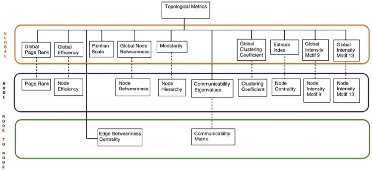
Hierarchy of multiple families of hypothesis testing.
Our relatively large number of high quality diffusion MRI data allows us to consider more related individuals than have been studied before for analyzing structural connectivity. We consider all possible pair-wise comparisons between the different kinships.
The rest of the paper is organized as follows: Estimation of brain structural connectivity section describes the diffusion MRI data we analyze. We describe how the data is processed to produce the anatomical brain connectivity information and networks. Methods section introduces the questions we address and our proposed approach using robust pattern recognition methods and multiple hypothesis testing, while controlling the FDR. Results section reports results for sex and kinship classification based on the brain connectivity matrices and network topology measures. Results section also presents results of hypothesis tests on the brain connectivity and brain topological network differences due to sex and kinship, as well as topological differences between human and random brain networks. Discussion section discusses the results, and some caveats and limitations. Conclusion section presents the conclusions of this work.
Estimation of brain structural connectivity
Diffusion MRI data acquisition and processing
The raw dataset consists of 4 T HARDI and standard T1-weighted structural MRI images, for 303 individuals (193 women and 110 men), between 20 and 30 years old (mean age: 23.5±1.9 SD years). From these subjects, we are able to form different pair-wise kinship relationships between identical twins (50), non-identical multiples (64 non-identical twins and a non-identical triplet, forming 67 pair-wise relationships), and non-twin siblings (35).1 In addition, there are 35 unrelated individuals, from whom we can obtain (35×34)/2=595 pairs of unrelated people, but we only choose at random 100 of them, to avoid unbalancing the number of pairs chosen for each class. In summary, we have 50+67+35+100=252 pairwise relationships for our kinship analysis.
All MR images were collected using a 4 T Bruker Medspec MRI scanner, with a transverse electromagnetic (TEM) head coil, at the Center for Magnetic Resonance, University of Queensland, Australia. T1-weighted images were acquired with an inversion recovery rapid gradient echo sequence (TI/TR/TE=700/1500/3.35 ms; flip angle=8°; slice thickness=0.9 mm, with a 2563 acquisition matrix). Diffusion-weighted images were acquired using single-shot echo planar imaging with a twice-refocused spin echo sequence to reduce eddy-current induced distortions. Imaging parameters were: TR/TE=6090/91.7 ms, 23 cm FOV, with a 128×128 acquisition matrix. Each 3D volume consisted of 55 2-mm thick axial slices with no gap, and a 1.79×1.79 mm2 in-plane resolution. We acquired 105 images per subject: 11 with no diffusion sensitization (i.e., b0 images) and 94 diffusion-weighted (DW) images (b=1159 s/mm2) with gradient directions evenly distributed on the hemisphere, as is required for unbiased estimation of white matter fiber orientations. Scan time was 14.2 min. Non-brain regions were automatically removed from each T1-weighted MRI scan, and from a b0 image obtained from the DWI dataset using the BET FSL tool.2 A trained neuroanatomical expert manually edited the T1-weighted scans to further refine the brain extraction. All T1-weighted images were linearly aligned using FSL (with 9 DOF3) to a common space, (Holmes et al., 1998), with 1 mm isotropic voxels and a 220×220×220 voxel matrix.
Raw diffusion-weighted images were corrected for eddy current distortions using the eddy current distortions correction FSL tool. For each subject, the 11 non-diffusion-weighted images (with no diffusion sensitization) were averaged and resampled and linearly aligned to a down-sampled version of the same subject, corresponding to a T1-weighted anatomical image (110×110×110, 2×2×2 mm). Averaged b0 maps were then elastically registered to the structural scan using an inverse consistent registration algorithm with a mutual information cost function (Leow et al., 2005), to compensate for high-field echo-planar imaging (EPI) induced susceptibility artifacts. This elastic registration further refines the linear intra-subject registration.
Thirty-five cortical labels per hemisphere (Table S1, in the supplementary material) were automatically extracted from all high resolution aligned T1-weighted structural MRI scans using FreeSurfer4 (Fischl et al., 2004). The output labels from FreeSurfer (1–35) for each hemisphere were combined into a single image. As a linear registration is performed within the software, the resulting T1-weighted images and cortical models were aligned to the original T1 input image space and down-sampled using nearest neighbor interpolation (to avoid intermixing of labels) to the space of the DWIs. To ensure tracts would intersect labeled cortical boundaries, labels were dilated simultaneously (to prevent overlap) with an isotropic box kernel of 5 voxels.
Tractography is performed by randomly choosing seed voxels of the white matter with a prior probability based on the fractional anisotropy (FA) value derived from the diffusion tensor model (Basser and Pierpaoli, 1996). We use a global probabilistic approach inspired by the voting procedure of the popular Hough transform (Duda and Hart, 1972; Gonzales and Woods, 2008). The tractography algorithm tests a large number of candidate 3D curves originating from each seed voxel, assigning a score to each, and returns the curve with the highest score as the estimated pathway. The score of each curve is computed from the agreement between the estimated curve and fiber orientations as derived from the Orientation Distribution Functions (ODFs) (Aganj et al., 2010). At each voxel of the DWI dataset, ODFs are computed using the normalized and dimensionless ODF estimator, derived for HARDI in Aganj et al. (2010), which is mathematically more accurate and also outperforms the original Q-Ball Imaging (QBI) definition (Tuch, Dec., 2004), e.g., it improves the resolution of multiple fiber orientations (Aganj et al., 2010).
As it is an exhaustive search, this algorithm avoids entrapment in local minima within the discretization resolution of the parameter space. Furthermore, the specific definition of the candidate’s tract score attenuates noise by integrating the real-valued local votes derived from the diffusion data.5 Further details of the method can be found in Aganj et al. (2010).
Elastic deformations obtained from the EPI distortion correction, mapping the average b0 image to the T1-weighted image, were then applied to the tracts 3D coordinates. To avoid considering small noisy tracts, tracts with fewer than 15 fibers were filtered out.
Computing connectivity matrices and brain networks
From the cortical labeling and tractography, symmetric matrices of connectivity (70×70) are built, one per subject. Each entry contains the number of fibers connecting each pair of cortical regions (Table S1) within and across each brain hemisphere. Connectivity matrices based on fiber counts should always be normalized to the [0, 1] range, as the number of fibers detected varies from individual to individual. In addition, there is a bias in the number of fibers detected by tractography that starts or end in any given cortical region, due to fiber crossings, fiber tract length, volume of the cortical region, and proximity to large tracts like the corpus callosum (Bassett et al., 2011; Hagmann et al., 2007, 2008; Jahanshad et al., 2011). However, there is no unique way to normalize the fiber tract count (Bassett et al., 2011).
We decided not to use the normalizations proposed in Bassett et al. (2011), and Hagmann et al. (2007, 2008), as they involve geometric measures including the volume of the cortical regions and the mean path length of fibers connecting each two regions. Instead, we considered three purely topological normalizations, since, as in Gong et al. (2009), we want to find pure topological network differences due to, e.g., sex and kinship:
| (1) |
| (2) |
| (3) |
where, aij represents the entries in the original fiber count matrix, A, and wij the entries (weights) of the now normalized 70×70 connectivity matrix, W.
Eq. (1) (used in our previous work, Jahanshad et al., 2011) normalizes the fiber count for each pair of regions by the total number of fibers in the entire brain, reducing variability among the connectivity matrices due to differences in the total number of fibers found. In practice, this normalization can provide biased weights, since it does not take into account that a higher number of fibers will be found in some regions, e.g., in the vicinity of the corpus callosum, and also more fibers would be counted in cortical regions with larger areas (Bassett et al., 2011; Hagmann et al., 2008).
Eq. (3), first proposed by Behrens et al. (2007) in the context of tractography, can be interpreted as the probability of connecting cortical regions i and j, given that there are aij fibers between them and there are Σj aij fibers available on cortical region i. Eq. (2), (Crofts and Higham, 2009), divides the number of fibers between any two cortical regions by the geometric mean of the number of fibers leaving either region. The assumption here is stronger than that of Eq. (3), as it assumes the same total number of fibers on each pair of brain regions. This can lead to bias due to large differences in the total number of fibers on each region (locally), but it should be correct on average (globally). An equivalent normalization was used in Gong et al. (2009), where instead of the geometric mean, they used an arithmetic mean, averaging wij and wji on Eq. (3).
Eqs. (1) and (2) lead to undirected connectivity graphs, which are typical in structural brain connectivity analysis. Eq. (3), on the other hand, leads to directed graphs (digraphs). To see this, note that in general Σiaij ≠ Σjaij, i.e. the total number of fibers on cortical regions i and j can be different on either side of the connection, hence, in general, wij ≠ wji on Eq. (3). Normalizations (1)-(3) are further modified as , where wij is defined as indicated in Eqs. (1)-(3), in order to reduce the differences among different connectivity matrices (different subjects), thereby making max{wij}=1. Eqs. (2), (3), modulated by max{wij}, reduce significantly the mean effect of brain size differences between men and women (see the regression analysis in Appendix A), which is a known confounding factor in analyses of sex differences (Leonard et al., 2008).
Here, we work with the normalization provided by Eq. (3),6 because it reduces the effect of brain size. Connectivity matrices are asymmetric–this coming from the normalization and not from the tractography results. This is beneficial as it uses all available entries in the matrix, while traditional symmetric matrices, as obtained from the other two normalizations, only use half of the matrix to store network information. This extra information is not an artifact of the normalization–it provides more information about differences between two connected brain regions. Two cortical regions are connected by the same number of fibers, but the proportion of fibers dedicated to that particular connection can be very different within each cortical region. For instance, consider the case where cortical region i connects exclusively to region j, but region j connects not only to i, but also to many other regions. In terms of probability of connection, pij=1, pik=0, k≠j, since i connects exclusively to j (pij being the probability of connecting region i with region j). However, pji<1, and pjk≠0 for some k regions, satisfying in both cases Σi pij = Σj pjk = 1 (all the regions must be connected), hence, pij≠pji. In the general case, each cortical region connects to a different number of other cortical regions, so in general, pij≠pji, as on Eq. (3). We consider that capturing this asymmetry in the connectivity matrices W is important, and this is validated in the experimental results.
In summary, we derived 303, one per subject, normalized connectivity (network) 70×70 matrices W, by applying probabilistic tractography to HARDI at 4 T. These matrices provide our basis for studying anatomical brain connectivity, as described next.
Methods
The research lines addressed here (see the Introduction) are independent as they answer different questions and there is no interaction or inference among them. It is important to state the independence of these research lines, as it implies that there is no need for an overall FDR error control, other than the FDR control on each research line (Benjamini and Hochberg, 1995; Yekutieli, 2008). The first two research lines are addressed simultaneously using robust pattern recognition methods that extend well to unobserved data (Classification section). The last three research lines are going to be addressed using statistical hypothesis testing (non-parametric bootstrap), where the corresponding null hypotheses are stated as:
There are no differences in the connectivity matrix. Given that there are O(n2) weights on a connectivity matrix of n nodes, there are O(n2) local null hypothesis to be tested, one for each connection, forming a large family of hypothesis testing. As n=70 in our case, we could have up to 4900 hypotheses to test for differences in the connectivity matrices.7
There are no global topological differences between real networks and random networks. In general, we can have m global topological metrics (see Fig. 1 and Topological metrics section for details), forming a single family of hypothesis testing.
There are no topological differences, at any scale, on the directed networks due to sex or kinship (Fig. 1). Hence, we have m hypotheses to test at the global level, possibly m families of hypothesis at the node level (one for each global hypothesis), having each one O(n), n=70, null hypothesis to test for differences at each node, and several families of hypotheses at the node-to-node level, where each family corresponds to a topological metric at the node-to-node level (Fig. 1), and each family consists of O(n2) hypothesis to test, one for each pair of nodes.
The first two null hypotheses require only a single (albeit possibly large) family of hypothesis tests, while the last one requires several families of hierarchically related hypothesis tests, where families of hypotheses at the node-to-node level can consist of O(n2) local hypotheses (up to 4900 hypotheses in our case, n=70).
At the population level, we consider only average network differences in the connectivity matrix (research line 3, see Introduction), or in the topological metrics of the associated graphs (research line 5 in the Introduction), resulting from sex and kinship, as we know a priori that the variability between the connectivity matrices of individuals can be as large as the variability between the connectivity matrices within the same group (same sex or same kinship relationship)–an observation derived both from previous studies (Bassett et al., 2011), and from our own dataset.
We consider the two classes women and men, based on sex; and the four classes identical twins, non-identical multiples, non-twin siblings, and unrelated individuals, based on kinship relationships. These are used for classification at the individual (including pairs of individuals for kinship) level and for hypothesis testing at the group level.
Our analysis of kinship follows previous genetic studies of brain connectivity (Fornito et al., 2011; Jahanshad et al., 2010, 2011; Rubinov and Bassett, 2011; Thompson et al., 2001). One traditional line of analysis in genetic studies uses a classical twin design to compute intra-pair (or intra-class) correlations between measures of cortical gray matter density (Thompson et al., 2001), connectivity matrices (Jahanshad et al., 2010, 2011), or wavelets representing the connectivity matrices (Fornito et al., 2011), however, these correlation operations reduce the data to a single matrix of correlations, and heritability statistics for all pairs of subjects in the same group.
For kinship analysis, we work with the absolute value of the differences in the connectivity matrix and with network differences in the topological metrics considered, between pairs of individuals. These pair-wise differences are differences between pairs of identical twins, differences between pairs of non-identical multiples, differences between siblings who are not twins, and finally differences between pairs of unrelated people. We use pairwise differences within and across families, as they allow us to detect genetically-mediated effects in pairings with different degrees of known genetic affinity (Thompson et al., 2001).
To avoid losing pairs of subjects in the kinship analyses, we did not constrain the pairwise differences between individuals to be of the same sex, which in our study corresponds approximately to half the non-identical multiples considered. The statistical power of the tests of kinship differences might be reduced by the confounding effects of sex differences, but at the same time, we are also increasing the statistical power of the test (Winer, 1971), by considering a larger number of pairwise differences.
Classification
Here, we want to classify individual brain connectivity networks in terms of sex (women and men) and pairs of individuals in terms of kinship, using the connectivity matrices or the associated network topology metrics at the node or node-to-node level.
In classification, we encounter the multiple comparisons problem (MCP), which arises whenever we test multiple hypotheses simultaneously. If we do not correct for this, then the more hypotheses tested, the higher the probability of obtaining at least one false positive.
This can be dealt with in classification via n-fold cross-validation. In fact, cross-validation can be more effective than Bonferroni-type corrections (Jensen and Cohen, 2000), as it does not test on the same data used to derive the model. Here we use 10-fold cross-validation, a good trade-off between robustness to unobserved data and using as much data as possible to train the classifiers (Refaeilzadeh et al., 2009). In addition to cross-validation, we also use permutation tests (see Appendix A for details), to non-parametrically evaluate the null hypothesis that the classifiers might have obtained good classification accuracies just by chance (Ojala and Garriga, 2010). In this work, we use Support Vector Machine (SVM) classifiers, as they extend well to unobserved data, (Vapnik, 1998), and deal with the MCP problem by reducing the number of comparisons to the number of support vectors.
Given the high dimensionality (ℝn2, n = 70 nodes) of the brain connectivity networks and associated topological metrics consider here (see Topological metrics section for their full description), we use feature selection methods to reduce the effective dimensionality of the data. We call here feature, any of the connectivity or topological network differences at the node-to-node and single node levels. Feature selection methods can significantly improve classification accuracy, even for classifiers that exploit the higher discrimination possibilities in high dimensional spaces, such as SVMs (Guyon and Eliseeff, 2003; Vapnik, 1998). In general, there are three methods used for feature selection: filters, wrappers, and embedded methods (Guyon and Eliseeff, 2003). Filter methods employ ranking criteria such as the Pearson cross-correlation (used for example in Dosenbach et al. (2010)), Mutual Information, Fisher criterion, and so on, and a given threshold to filter out low ranked features. Wrappers use the classifier itself to evaluate the importance of each feature and explore the whole feature space using for instance, gradient based methods, genetic algorithms or greedy algorithms. Filter methods are very fast and independent of the selected classifier, however, they can lead to the selection of redundant features (Guyon and Eliseeff, 2003). They also disregard features with relatively small individual influence that can potentially have an influential effect as a group. Wrappers, on the other hand, can avoid redundant features and identify influential subgroups of features. However, they are computationally intensive, since the subset feature selection problem is NP-hard (Amaldi and Kann, 1998), and are strongly dependent on the classifier used (Guyon and Eliseeff, 2003). Embedded methods also use a classifier to evaluate the importance of subgroup of features. Hence, they are wrappers. However, they provide a trade-off between other wrappers and filter methods, in terms of computational efficiency and reduced number of features, since they introduce a penalty term that enforces small number of features (Guyon and Eliseeff, 2003).
An alternative to feature selection methods are dimension reduction methods such as Principal Components Analysis (PCA) and Independent Component Analysis (ICA). See Hartmann (2006), for a comparison of both methods in the context of machine learning. Here, we preferred feature selection methods, as the features in dimension reduction methods are in general functions of the original features,8 and cannot be associated to a unique “physical” feature in the original data space. In particular, we use the SVM-based embedded feature selection algorithm proposed by Guyon et al. (2002). When selecting features with a classifier there is a risk of “double-dipping,” i.e., training the feature selection algorithm and testing it with the same data, which leads to unrealistic high accuracies (over-fitting) that do not extend well to unseen data (Kriegeskorte et al., 2009; Refaeilzadeh et al., 2009). To avoid this, the feature selection algorithm uses 10-fold cross validation, 9 selecting the features that contribute more to classification, but that are also more stable across the different cross-validation sets of data (Kriegeskorte et al., 2009; Refaeilzadeh et al., 2009). In the proposed framework, feature selection algorithms extract the m ≪ n2 most relevant features from the digraph matrices taken as high dimensional vectors in ℝn2, n = 70, then use the m selected features to classify the reduced features in ℝm.
We tested classification performance using the following standard measures:
The overall classification accuracy.
The sensitivity and specificity.10
The balanced error rate (BER), which corresponds to the average of the errors on each class.
The area under the receiver operating characteristic (ROC) curve, which measures the probability that the classifier can actually discriminate the true class from the incorrect one(s).
The kappa statistic, which measures the agreement of the classifier with the labels taking into account the probability that the agreement has been obtained by chance. It uses the confusion matrix to make this assessment.
Permutation tests p-values, which non-parametrically assess the probability that the classification results were obtained by chance by estimating the null hypothesis distribution.
For space considerations, the confusion matrices were not included here, and can be found in the supplementary material.
Topological metrics
In addition to studying node-to-node connections, e.g., just the entries of the matrix W as stand-alone features, we would like to consider features that indicate higher levels of interactions between the studied regions.
As we do not know a priori which topological metrics would provide statistically significant differences between different classes of brain connectivity networks, we have to limit ourselves to a few selected ones, to control the FDR error within each research line. We consider 11 representative topological metrics at the global, node, and node-to-node level (Fig. 1). While some have been studied for brain networks, all these topological features have found relevance in other disciplines, such as social networks (Easley and Kleinberg, 2010), and provide interesting insights into the overall organization of the brain.
Node-to-node level
At the node-to-node level we consider the edge betweenness centrality (EBC), a new subgraph based centrality (SGC), and the communicability measures (COM) (Estrada, 2010; Estrada and Higham, 2010). The weighted edge betweenness centrality is defined as (Rubinov and Sporns, 2010),
| (4) |
where is the number of shortest paths between nodes h and k that contain edge ij and ρhk is the number of shortest paths between h and k. EBC measures the fraction of all shortest paths in the network that contain edge ij, and hence, the importance of each edge in the communication among cortical regions.
To understand the subgraph centrality (SGC) and communicability (COM) measures (Estrada, 2010; Estrada and Higham, 2010), let us first decompose the connectivity matrix as W = ΛW + W̃, where ΛW is a diagonal matrix, with non-zero entries corresponding to the diagonal of W, and W̃ is the resulting matrix of making zero the diagonal of W. Notice that ΛW contains the self-connections of each node, while W̃ the connections between each pair of nodes. Let us define (Estrada, 2010; Estrada and Higham, 2010),
| (5) |
where, In is the identity matrix of size n × n and we have used the definition of the exponential of a matrix. The product w̃ih1 w̃h1h2…w̃hk−1j measures the strength of the walk (i, h1, ots, hk−1, j) of length k, between nodes i and j. A walk is a list of connected nodes that can be visited more than once, contrary to a path, where the nodes are visited at most once. Hence, the elements of W̃k account for the strength of all possible walks of length k between nodes i and j. Also, the entries of P̃ correspond to the weighted sum of the strength of all possible walks of length one and higher, between nodes i and j, providing thus a measure of how strong the communication is between them (communicability, Estrada and Higham, 2010; Estrada, 2010). Given that the number of walks increases with length, the weight k! is selected to compensate for this effect, penalizing long walks.
Now, we can define (Estrada, 2010; Estrada and Higham, 2010),
| (6) |
Hence, the subgraph centrality of a node SGCi corresponds to the communicability of a node with itself, while COMij corresponds to the communicability between two different nodes i≠j.
Notice that the diagonal of matrix P̃ is a weighted sum of all closed walks (information transfer) of lengths two and higher around each node. The information provided by the closed walks of length zero in the connectivity matrix (ΛW) is lost, however, since it is not used anywhere. To recover it, we define here P = P̃ + ΛW as the generalized communicability matrix, since it provides all possible communications among all nodes of length zero and above, without including self-loops other than the one in the starting node itself.
The communicability matrix has no zero entries, except along the diagonal, which implies 4900–70 (4830) hypothesis tests for our data (n=70), one for each non-zero entry. Hence, a spectral analysis of the communicability matrix can be performed, (Crofts and Higham, 2009; Estrada, 2010), to obtain a family of tests of order O(n), where n are the number of eigenvalues of the communicability matrix. In particular, the above defined matrix COM can be decomposed in terms of its eigenvalues and eigenvectors as
| (7) |
where λk are the eigenvalues of COM, and vk its eigenvectors, k=1,…,n.
Global and node levels
The undirected network efficiency (E) and clustering coefficient (C), have been previously reported as indicative of sex and age differences (Gong et al., 2009). Here, we use the directed weighted versions, defined as (Rubinov and Sporns, 2010),
| (8) |
| (9) |
where, n represents the number of nodes, dij the weighted directed shortest path length between nodes i and j, and Ni the neighborhood of node i (nodes connected to node i by a single link). Network efficiency measures how fast information can be transmitted in the network, globally (E), and locally at each node (Ei). The clustering coefficient measures how much nodes in a graph tend to cluster together, globally (C) and locally at the node level (Ci). Basically, the directed weighted clustering coefficient measures the probability that neighbors of a node are also connected between themselves, hence, forming clusters around a node.
Additional traditional topological metrics at the global and node levels are the weighted directed betweenness centrality (BC), weighted modularity (Q), and motifs (Rubinov and Sporns, 2010). The weighted directed node betweenness centrality is defined as (Rubinov and Sporns, 2010),
| (10) |
where, represents the number of shortest paths from nodes h and j that go through i, and ρhj the total number of shortest paths between h and j. The directed weighted node betweenness centrality measures how important each node is in the communication between neighboring nodes.
The weighted modularity (Q) is defined as (Rubinov and Sporns, 2010),
| (11) |
where the network is assumed to be fully subdivided into non-overlapping clusters or modules (M), with Mi being the module that contains node i, and δMi, Mj=1 if Mi=Mj and zero otherwise. This is a global measure of the modularity of the network, that is, how tightly nodes are connected within a module. Identifying modules is of course a first step in analyzing the structure of the brain at a higher scale. This global topological measure has a local hierarchical representation, where we can have hierarchies of modules (clusters). Modules can be found using, for instance, the Louvain hierarchical modularity algorithm (Blondel et al., 2008), a graph partitioning algorithm that tries to find the partition maximizing Eq. (11). Since graph partitioning is in general an NP-complete problem, the Louvain algorithm computes a local optimum by greedy optimization. Fig. S1, in the supplementary material, is an example of hierarchical module graph partitioning using the full dataset.
Network motifs (Onnela et al., 2005; Rubinov and Sporns, 2010), are also topological metrics that measure the intensity or frequency of certain subgraph patterns such as directed connections forming a triangle, a square, etc. The intensity of a weighted motif (Fmotif) is defined as,
| (12) |
where motif indicates a given motif, h a node, the set of nodes forming the motif at node h, and |Lmotif| the number of directed links in the motif. Motifs are considered the building blocks of information processing in the network and can be measured globally (Fmotif) or locally at the node level . Fig. S2, in the supplementary material, shows the 13 possible directed motifs of size three.
New topological metrics, while popular in studies of other network data, have not yet been used for anatomical brain networks. We will also consider the PageRank (PR) (Easley and Kleinberg, 2010; Lohmann et al., 2010; Shepelyansky and Zhirov, 2010) and the Rentian scale, (Bassett et al., 2010) here. In essence, the PageRank (critical in Internet network analysis and search engines performance) is a measure of how important a node is, based on the importance of its neighbors. Hence, this is a recursive metric that starts with all the nodes having the same measure of importance. More formally (Brin and Page, 1998),
| (13) |
where again n is the number of nodes, Ni the neighborhood of node i, α is a damping parameter set in the [0,1] range, and t=1,2,… the iterations until convergence, defined as |PR(t+1)−PR(t)|≤silon, for some small number ε. The PageRank tries to identify nodes that are influential in the network, not only because they have many connections with other nodes, but also because those neighboring nodes are influential themselves. This may be a better definition of node importance than traditional hubs, which account only for the number of connections of a node (node degree).
The Rentian scale11 is a measure of the wiring modular complexity of the network that is self similar (fractal) at different scales. This is a metric of modularity that differs from the previous one (Q) in that it is hierarchically represented as modules within modules at different network scales. More formally (Bassett et al., 2010),
| (14) |
where EC is the number of external connections to a module, k a proportionality constant, N the number of nodes in the module, and r the Rentian exponent. Here, we use the physical Rentian scale, which uses the physical coordinates of the brain cortical regions. In order to avoid introducing the obvious differences in the brain size due to sex, we use the same physical coordinates for all brain cortical regions, corresponding to a single brain.
The Rentian scale is computed as the mean Rentian exponent on Eq. (14), by partitioning the network into halves, quarters, and so on in physical space, providing EC and N values at different scales. The constant k and Rentian scale r are computed by least squares minimization of the linearized Eq. (14), log(EC)=log(k) + r log(N) for all values of EC and N obtained from such partition (Bassett et al., 2010).
Some node-to-node topological metrics can lead to global metrics. For instance, the trace of ΛP̃ is a global measure of node importance called the Estrada index. The EBC can also be made global, by averaging it over the entire network. Nevertheless, this kind of large averaging might destroy local differences at the edge level and will not be considered here.
FDR error control
Single family of hypothesis testing
To control the FDR for the single families of hypothesis corresponding to the research lines “are there any global topological differences between real brain connectivity networks and random networks;” and “are there any mean differences between connectivity matrices due to sex and kinship?,” we use here the linear step-up algorithm of Benjamini–Hochberg (Benjamini and Hochberg, 1995), hereafter BH-FDR. The BH-FDR algorithm has been applied in many recent multiple hypothesis testing studies, including brain connectivity analysis (Gong et al., 2009; He et al., 2007; Jahanshad et al., 2010).
Other approaches to control the FDR in multiple hypothesis testing that are less conservative than the BH-FDR algorithm have been proposed in the literature (Benjamini and Hochberg, 2000; Benjamini and Yekuteli, 2001, 2005; Storey, 2002; Storey et al., 2004; Westfall et al., 1997), but they require either independence of the hypotheses being tested or a known correlation structure (Reiner-Benaim, 2007). The BH-FDR algorithmis still the most widely used, as it is simple and it controls the FDR for normally distributed tests with any correlation structure (Benjamini et al., 2009; Reiner-Benaim, 2007). As we are working with mean differences in a large number of connectivity matrices, we can assume that the mean follows a normal distribution, by the central limit theorem (Fisher, 2011). Hence, the simple BH-FDR error control is quite appropriate here. For completeness, we provide here the basic BH-FDR algorithm (Benjamini and Hochberg, 1995; Yekutieli, 2008):
Algorithm 1. BH-FDR
Sort in increasing order all the p-values of the null hypothesis: p1≤p2≤…≤pL.
Let r = maxi{pi ≤ q/L}, define the threshold pth = pr. If no r could be found, define pth = q/L (pure Bonferroni).
Reject all null hypothesis with pi ≤ pth.
where, L is the number of null hypothesis and q the desired family-wise confidence level.
Multiple families of hypothesis testing
As explained before, we have a tree of topological metrics at different levels of resolution (Fig. 1). Hence, we need to test each topological metric at the global, node-to-node, and node levels. Nevertheless, testing the topological metrics at the node-to-node and node levels consists of testing families of hypothesis of sizes O(n) and O(n2), respectively, where n corresponds to the number of nodes in the network. Hence, we have multiple families of hypothesis testing and we need to control the overall FDR on each of the proposed research lines.
The FDR error control has been limited so far to a single family of multiple hypothesis testing. The implicit assumption in many large studies has been that there is no need to control the FDR when multiple families of hypotheses are being performed on the same dataset, other than the FDR control on each family of hypotheses (Yekutieli, 2008). However, in general, the FDR control separately applied to each family of hypothesis does not imply FDR control for the entire study (Benjamini and Yekutieli, 2005; Yekutieli, 2008). If a separate control of the FDR is performed on each family of hypotheses, then the overall FDR error corresponds to the sum of FDR errors of each family, which can quickly make the overall p-value of the study too large to be of any use. As we compare different topological metrics at different levels, we have different families of multiple hypothesis tests that require overall control of the FDR for each research line.
To control the overall FDR error, we proceed in a hierarchical way, testing from lower to higher resolutions, as suggested by Yekutieli (2008) and Yekutieli et al. (2006). This strategy makes sense since it avoids testing first at higher resolutions, where the number of hypotheses to be tested on each family could go up to 4900 (n=70). If the fraction of null rejections is small, then the FDR error control becomes as stringent as Bonferroni correction (Yekutieli, 2008), which significantly increases the chance of not rejecting any false null hypotheses (false negatives or Type II error).
Fig. 1 shows the tree of possible hypotheses while testing the topological differences due to sex and kinship at three levels: global, node (cortical regions), and node-to-node (shortest paths and communicability). The dashed lines in Fig. 1 indicate that the higher resolution hypotheses are only tested if the parent null hypothesis was rejected, as indicated by Yekutieli (2008).
A specific example (see Fig. 1) is the communicability matrix (COM), which contains O(n2) non-zero entries, and hence, O(n2) hypotheses to test. We can test instead its eigenvectors (Eq. (7)), which requires only O(n) hypothesis tests to determine if COM might be significant.
Let H0 = { , i = 1, … L0} be the set of hypothesis to be tested at the lowest resolution level, and Hk = { , i = 1,…Lk, j ∈ Hk − 1} be the set of hypothesis at resolution levels k=1,…,K. In our case, K=2, where K=0 corresponds to the topological metrics at the global level, K=1 to the topological metrics at the node level, and K=2 to the topological metrics at the node-to-node level (again, see Fig. 1). Hence, we have a hierarchy of hypotheses, where the FDR error is controlled at each level simultaneously on all families of hypotheses, using the BH-FDR algorithm (see Single family of hypothesis testing section), imposing as mentioned above the condition that higher resolution hypotheses are tested only if the parent hypothesis has been rejected
If the p-values corresponding to the hypotheses being tested are independently distributed, true null hypotheses p-values have uniform distributions, and for false null hypotheses, the conditional marginal distribution of all the p-values is uniform, orstochastically smaller than uniform (Yekutieli, 2008). In such cases, the overall FDR for the whole tree of hypotheses is bounded to FDR ≤2δq, where q is the family-wise confidence level and δ≈1.0 for most cases, but can be as large as δ≈1.4 for thousands of hypothesis with few discoveries. Hence, controlling the FDR on each level at q=0.05 will bound the overall FDR at 0.1 in most cases or at 0.14, when thousands of hypotheses are tested and the number of discoveries is relatively small compared to the number of hypothesis tested (see Yekutieli, 2008).
Testing for all the required conditions on the p-values and computing δ to bound the overall FDR as defined before, are daunting tasks that have been tackled in the past by modeling and multiple simulations with synthetic data (Reiner-Benaim et al., 2007; Yekutieli, 2008). Instead, we can use the fact that the bound of the overall FDR is the sum over k=0,…,K of the bounds for the FDR at each level, FDR(k) (Yekutieli, 2008; Yekutieli et al., 2006). Hence, the overall tree FDR ≤(K + 1)q, where K+1 is the number of levels in the tree. Here K=2, hence, FDR ≤3q=0.15, for a family-wise confidence level of 0.05 at each level, which is quite close to the predicted (most conservative) theoretical overall bound with δ=1.4.
Screening
Despite the overall control of the FDR described before, for large studies, it is quite possible that the BH-FDR control would become equivalent to a simple (too conservative) Bonferroni correction, and no single null hypothesis could be rejected (Benjamini and Yekutieli, 2005). Most large studies, e.g., the expression levels of thousands of genes in microarrays, nowadays use screening methods to reduce the number of hypotheses tested, improving the overall statistical power of the FDR control, especially when the fraction of rejections of the null hypothesis is small (Benjamini and Yekutieli, 2005). Screening to eliminate some uninteresting hypotheses is valid, so long as the null hypothesis of the screening method is independent of the null hypothesis being tested (Yekutieli, 2008). Since the null hypothesis in most tests is that mean differences are zero, a valid screening method is an ANOVA single effects F-ratio screening (Reiner-Benaim et al., 2007), in which the null hypothesis depends on the variance of the data (see details in Appendix A).
In addition to reducing the number of hypotheses to be tested, it has been also proposed to use thresholds on the connectivity matrices themselves to get rid of noisy connections, avoiding thus unnecessary tests on those connections. To avoid ad-hoc thresholds, we screen the connectivity matrix using a set of increasing thresholds that produce different connectivity matrices at different sparsity levels (Achard and Bullmore, 2007; Bassett et al., 2008; Bullmore and Bassett, 2011; Rubinov and Sporns, 2010). This data screening technique reveals statistical differences at different levels of sparsity that are not seen with a single ad-hoc threshold (Gong et al., 2009). Optionally, a single robust threshold can be used on the connectivity matrices themselves, using the BH-FDR error control (Abramovich and Benjamini, 1996). Here, we screen the normalized connectivity matrices with thresholds in the [0, 0.05] range,12 as in Gong et al. (2009) given that the BH-FDR based threshold is too stringent and may miss important discoveries. Fig. S3 illustrates how these thresholds affect the sparsity of the thresholded matrices.
Here, we use then the simple screening method of thresholding the connectivity matrices at different sparsity levels proposed by Achard and Bullmore (2007), Bassett et al. (2008), Bullmore and Bassett (2011), and Rubinov and Sporns (2010), given its simplicity and independence of the hypothesis being tested. Then, we apply an ANOVA single effects F-ratio screening test to eliminate remaining uninteresting hypotheses (see Appendix A for details). This kind of selective inference has not yet received proper theoretical or practical consideration in the context of screening uninteresting hypotheses and the less obvious connection between the screening test and the follow-up one (Benjamini et al., 2009; Reiner-Benaim, 2007). Better FDR error control algorithms are needed, especially for cases where the number of null hypotheses is large and the FDR methods reduce to a simple Bonferroni correction.
Bootstrapping
We need to describe how are we going to compute the p-values that the BH-FDR error control requires. As we are working with average connectivity and topological network differences between different groups of individuals (including pairs of individuals), then by the central limit theorem, those averages should asymptotically follow a Gaussian distribution (Fisher, 2011). Nevertheless, there could be some small variations from the Gaussian distribution on real finite samples, so we use a non-parametric approach. Bootstrapping can improve the reliability of inference compared with conventional asymptotic tests (Davison and MacKinnon, 1999). We use bootstrapping with replacement to obtain 20,000 samples of the mean for each metric, scale, and class. The p-values (p) required by the BH-FDR error control can be easily computed from the bootstrapped distribution of the mean differences,
| (15) |
where B is the number of bootstrapped samples, c=1 for single-tailed tests, c=2 for double-tailed tests, si are the bootstrapped sample differences, and I(si) the frequency of those samples. Sample differences are for instance differences in the clustering coefficient at a given brain region (node) i, or differences in the communicability matrix taken as a columnvector at the entry i, due to sex. As in Gong et al. (2009), we consider positive and negative differences in the connectivity matrices and topological metrics of the associated digraphs for both sex and kinship differences, so we will use one-tailed p-values.
Z-scores global topological metrics
As the global topological metrics of the brain connectivity networks and their corresponding random networks are independent, the Z-score of their differences is
| (16) |
where M̅ indicates the mean of metric M and M̅R the mean metric for the corresponding random network. Here we use a parametric t-test, as there are enough samples of the population to assume Gaussianity, and being consistent with previous results comparing real and random networks (Boccaletti et al., 2006; Rubinov and Sporns, 2010).
Results
We show here the results obtained from the 303 HARDI-derived connectivity matrices, with a formal statistical analysis of the topological features as described before. For space considerations, the detailed lists of features are presented in the supplement, with corresponding p-values and mean differences.
The figures in the next sections showing the features selected by the machine learning methods described in Classification section are color coded according to the score provided by the feature selection algorithm. This score accounts for the effects of each feature on the classification accuracy and its stability across the n-fold cross-validation runs (see more details on the tools employed in Appendix A). We do not indicate here which are the top ranked features, since all the features selected are important for classification purposes, even if they ranked the lowest. For instance, if we only take the 10 top ranked features and use them for classification, the performance would be relatively poor.
Figures in the next sections showing the statistically significant features found in hypothesis testing (FDR error control section) are color coded according to their Z-score and the sign of the difference, magenta for positive and cyan for negative. As the sign of the difference depends on the order of the operands, we specify in the corresponding text and on each figure what is the meaning of each color.13
Classification
Tables S2–S4 compare the classification results for the three node-to-node level metrics considered here, the “raw” connectivity matrices, generalized communicability matrix (P), and edge betweenness (EBC), using the three normalizations indicated in Estimation of brain structural connectivity section. The performances of sex classification for the connectivity matrices, generalized communicability, and edge betweenness, using Eq. (3), are 93%, 92.2%, and 92.5%, respectively. The corresponding performances for Eq. (1) are 88.1%, 88.1%, and 93.7%, respectively, and for Eq. (2) are 89.9%, 88.3%, and 80.7%, respectively. The performances of kinship classification for the connectivity matrices, generalized communicability, and edge betweenness, using Eq. (3), are 88.5%, 88.5%, and 87.3%, respectively. The corresponding performances for Eq. (1) are 89.7%, 85.8%, and 75.2%, respectively, and for Eq. (2) are 87.4%, 83.6%, and 75.5%, respectively.
Notice, that in some cases, Eq. (1) produces slightly better classification results than Eq. (3), however, as indicated in Appendix A, only Eqs. (2)-(3) reduce significantly the confounding effects of brain size. In addition, Eq. (3) produces the best overall classification results, considering all the classes and topological metrics.
Classification performance was just slightly better than chance for all topological metrics at the node level (Fig. 1), and hence, they were not compared here using Eqs. (1)-(3). Next sections show in more detail the classification results using Eq. (3).
Connectivity matrices
We start with the classification results when the “raw” connectivity matrices are used, one per individual and one per pair of individuals. Tables 1 and S5 (for the confusion matrix, provided in the supplementary material) compare sex classification performance using all features (probabilities of connection between the n=70 cortical regions) of the connectivity matrix against feature selection. Feature selection greatly improves classification performance–the selected features provide more information to distinguish between sexes. Overall, classification accuracy improved from 49.5% using up to 2763 features of the connectivity matrices, to 93% after feature selection that reduced the number of features to 297. According to our permutation tests, the probability of achieving this classification performance by chance is 0.001 or lower. Fig. 2a shows the features that provide the best classification results for sex, in the raw connectivity matrix. Table S7 in the supplement lists the selected features in more detail.
Table 1.
Sex classification performance (see Classification section) obtained from the connectivity matrix (node-to-node level). We observe significantly improved results when feature selection is incorporated.
| Test | All features (2763) | Feature selection (297) |
|---|---|---|
| Classification accuracy (%) | 49.5 | 93.0 |
| Sensitivity (%) | 56.5 | 95.5 |
| Specificity (%) | 37.3 | 88.5 |
| Balanced error rate (BER) | 0.5313 | 0.0797 |
| Area under the ROC curve | 0.473 | 0.9203 |
| Kappa statistic | −0.067 | 0.8470 |
| p-value | – | 0.001 |
Fig. 2.

Selected features on the connectivity matrix for a) sex and b) kinship classification.
The feature selection algorithm selected 70 inter-hemispheric features as influential for sex classification purposes and about the same number of features on the left (113) and right (114) hemispheres (Fig. 2a).
Tables 2 and S6 (for the confusion matrix, in the supplementary material) compare kinship classification performance using all features of the connectivity matrix versus feature selection. Here, the overall classification accuracy improved from 63.5% using up to 2763 features of the connectivity matrix to 88.5% using the 250 features, automatically selected by feature selection. Permutation tests indicate that the probability of arriving to this classification performance by chance is equal or below to 0.001. Fig. 2b shows the features that provide the best classification results for kinship, in the connectivity matrix. Table S8 in the supplementary material list the corresponding selected features in more detail.
Table 2.
Kinship classification performance (see Classification section) obtained from the connectivity matrix (node-to-node level).
| Test | All features (2763) | Feature selection (250) |
|---|---|---|
| Accuracy (%) | 63.49 | 88.5 (0.010) |
| Sensitivity identical twins (%) | 28.0 | 80.4 |
| Specificity identical twins (%) | 88.2 | 94.5 |
| Sensitivity non-identical twins (%) | 46.8 | 86.2 |
| Specificity non-identical twins (%) | 77.8 | 96.0 |
| Sensitivity siblings (%) | 28.6 | 72.2 |
| Specificity siblings (%) | 92.5 | 97.4 |
| Sensitivity unrelated people (%) | 100.0 | 99.9 |
| Specificity unrelated people (%) | 88.3 | 96.9 |
| BER | 0.3671 | 0.1535 (0.016) |
| ROC area | 0.759 | 0.904 (0.01) |
| Kappa | 0.4796 | 0.838 (0.017) |
| p-value | – | 0.001(0) |
The feature selection algorithm selected 59 inter-hemispheric features as influential for kinship classification purposes and about the same number of features selected on the left (97) and right (94) hemispheres (Fig. 2b).
Topological metrics
The best results at the node level correspond to the clustering coefficient and for sex classification, as indicated in Table 3. Overall classification accuracy improved from 55.4% using the clustering coefficient on all 70 nodes to 62.7% using the 53 (not a significant reduction) nodes selected using automatic feature selection.
Table 3.
Sex classification performance (see Classification section) using the clustering coefficient (node level).
| Test | All features (70) | Feature selection (53) |
|---|---|---|
| Classification accuracy (%) | 55.4 | 62.7 |
| Sensitivity (%) | 64.8 | 89.6 |
| Specificity (%) | 37.0 | 25.2 |
| Balanced error rate (BER) | 0.4983 | 0.4261 |
| Area under the ROC curve | 0.502 | 0.7309 |
| Kappa statistic | 0.0035 | 0.5214 |
| p-value | – | 0.001 |
On the other hand, good classification results were obtained for sex and kinship using the node-to-node topologicalmetrics: edge betweenness centrality (EBC) and the generalized communicability matrix (P), respectively. The results from the generalized communicability matrix are slightly better than those using EBC for sex, while those from EBC are slightly better for kinship. Hence, we present here the best classification performances.
Tables 4 and S9 in the supplement (confusionmatrices) showthe sex classification performance using the generalized communicability matrix. For comparison purposes, we also compute the classification performance using FDR (Abramovich and Benjamini, 1996) to select the most statistically significant elements of the generalized communicability matrix at the q=0.05 level. Sex classification accuracy improved from 51.8% using all 4900 features of the generalized communicability matrix to 92.2%14 using the 301 features automatically selected by feature selection. The overall accuracy of sex classification degraded to 46.2% using the 935 features selected by FDR thresholding.
Table 4.
Sex classification performance (see Classification section) using the generalized communicability matrix (node-to-node level).
| Test | All features (4900) | FDR thresholding (935) | Feature selection (298) |
|---|---|---|---|
| Accuracy (%) | 51.8 | 46.2 | 92.2 |
| Sensitivity (%) | 58.0 | 45.1 | 93.7 |
| Specificity (%) | 26.4 | 30.9 | 89.6 |
| BER | 0.5268 | 0.5780 | 0.0835 |
| ROC area | 0.473 | 0.429 | 0.917 |
| Kappa | −0.054 | −0.139 | 0.832 |
| p-val | – | – | 0.001 |
Tables 5 and S10 in the supplement show the kinship classification performance using edge betweenness centrality, where as before, we included the classification performance using FDR for feature selection. The overall kinship classification accuracy improved from 57.1% using 2388 features of P to 87.3% using the 251 features selected by feature selection. The overall accuracy of kinship classification degraded to 32.1% using the 1031 features selected by FDR thresholding.
Table 5.
Kinship classification performance (see Classification section) using edge betweenness centrality (node-to-node level).
| Test | All features (2388) | FDR thresholding (1031) | Feature selection (251) |
|---|---|---|---|
| Accuracy (%) | 57.1 | 32.14 | 87.3 |
| Sensitivity identical twins (%) | 22.0 | 16.0 | 76.4 |
| Specificity identical twins (%) | 84.7 | 85.6 | 97.0 |
| Sensitivity non-Identical Twins (%) | 40.3 | 31.3 | 86.7 |
| Specificity non-Identical Twins (%) | 82.2 | 71.9 | 92.0 |
| Sensitivity siblings (%) | 25.7 | 11.4 | 70.9 |
| Specificity siblings (%) | 91.2 | 90.8 | 97.5 |
| Sensitivity unrelated people (%) | 97.0 | 48.0 | 98.8 |
| Specificity unrelated people (%) | 83.6 | 53.9 | 96.1 |
| BER | 0.5636 | 0.8870 | 0.1677 |
| ROC area | 0.708 | 0.511 | 0.8945 |
| Kappa | 0.3843 | 0.0234 | 0.820 |
| p-val | – | – | 0.001 |
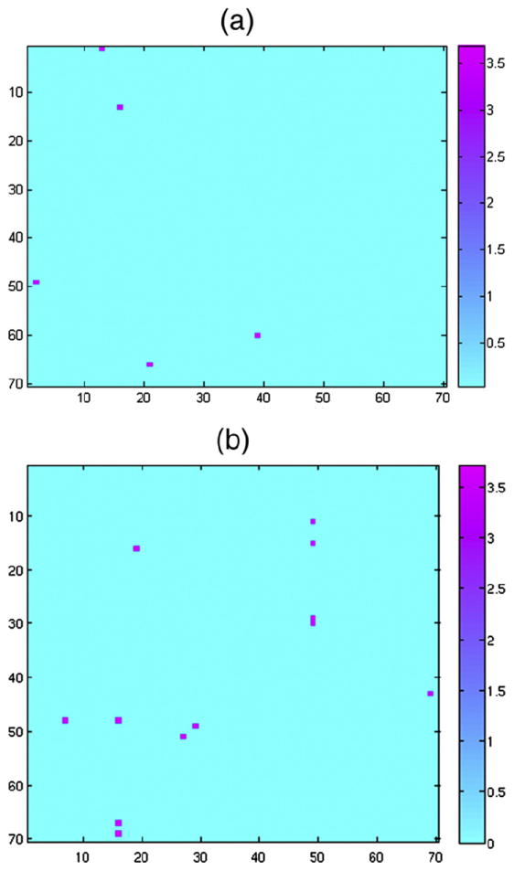
Fig. 3a shows the 301 features (entries) of the generalized communicability matrix that provide the best classification results for sex (listed in more detail on Table S11), while Fig. 3b shows the 251 features (edges) of the EBC metric that provide the best classification results for kinship (listed in more detail on Table S12). The 301 best entries of the communicability matrix for sex classification represent weighted walks of different lengths (or subgraphs, see Node-to-node level section) centered on the connections indicated on Fig. 3a.
Fig. 3.

a) Selected features on the communicability matrix for sex classification, b) selected features on the edge betweenness centrality matrix for kinship classification. Color code corresponds to the score given by the feature selection algorithm.
The total number of automatically selected entries of the communicability matrix was distributed as 99 centered on inter-hemispheric connections, 116 centered on the left hemisphere, and 86 on the right hemisphere. On the other hand, the 251 entries of the EBC for zygosity classification represent (see Node-to-node level section) the importance of each connection in the connectivity matrix in terms of shortest paths using such connections. In particular, the selected entries of the EBC were distributed as (Fig. 3b) 51 inter-hemispheric, 94 in the left hemisphere, and 107 in the right hemisphere.
Even though classification with cross-validation does not require Bonferroni correction, the p-values of the permutation tests do require correction, as each permutation test corresponds to testing the null hypothesis that the reported classification performance was obtained by chance (Ojala and Garriga, 2010). In these two lines of research (sex and kinship), we performed permutation tests for the 11 proposed topological metrics (not all shown here) indicated in Fig. 1 at the node and node-to-node levels, plus the permutation tests performed to compare Eqs. (1)-(3) and those to compare the generalized communicability matrix with the communicability matrix (also not shown for space reduction). Hence, we did in total 13 permutation tests for sex and 13 for kinship. The BH-FDR correction keeps the overall false discovery rate for the permutation tests to 0.001, since all tests rejected the null hypothesis at this confidence level.
Hypothesis testing
Connectivity matrices
We now present the results of hypothesis testing on differences in the connectivity matrix due to sex and kinship. Prior work on connectivity matrices for differentiating sex and kinship classes have focused on just a few connections (10) (Jahanshad et al., 2011). Previous work also did not consider all possible pair-wise comparisons between identical twins, non-identical multiples, non-twin siblings, and unrelated subjects.
Sex Differences
Fig. 4 shows the 36 statistically significant sex differences found in the connectivity matrices after BH-FDR error control, requiring a Z-score 1.75 or higher (p-value of 0.0405 or lower, for a single tailed normal distribution). The color map indicates where the probability of connection is higher for women (magenta) than for men (cyan). As seen in this figure, on average, women have higher brain connectivity than men in both hemispheres, on the directed connection pairs shown. Fig. 4 also shows that women have higher inter-hemispheric connectivity than men, in agreement with Jahanshad et al. (2011). Nevertheless, men have some higher probabilities of connection than women, mainly on the right hemisphere (Fig. 4). Table S13 in the supplement shows in more detail each pair of connection statistics (36) with their means and p-values. The first five largest relative differences with the lowest p-values were in the following connections: Pars Opercularis–Post Central and Frontal Pole–Caudal Anterior Cingulate, in the left hemisphere, Inferior Parietal–Corpus Callosum, in the right hemisphere, and the inter-hemispheric connections Cuneus (right)–Lateral Occipital (left) and Inferior Parietal (left)–Corpus Callosum (right).
Fig. 4.

Z-score sex differences from the connectivity matrix. The color map indicates where the probability of connection is higher for women (magenta) or for men (cyan). Color code corresponds to the score given by the feature selection algorithm.
Kinship differences
Fig. 5 shows the statistically significant differences between a) identical twins and non-identical multiples, b) identical twins and non-twin siblings, c) identical twins and unrelated pairs of individuals, d) non-identical multiples and non-twin siblings, e) nonidentical multiples and unrelated pairs of individuals, and f) non-twin siblings and unrelated pairs of individuals; covering thus all possible pair-wise comparisons between these four groups. The reported differences have a Z-score of 2.67 or higher as required by the FDR error control overall possible pair-wise comparisons. As may be expected for a genetically influenced trait (Thompson et al., 2001), greater differences are found between unrelated pairs of individuals and siblings than between non-twin siblings and twins. Also, greater differences are found between siblings and twins than between identical twins and non-identical multiples. The color map indicates where the differences are higher for the first group (magenta) or for the second (cyan).
Fig. 5.
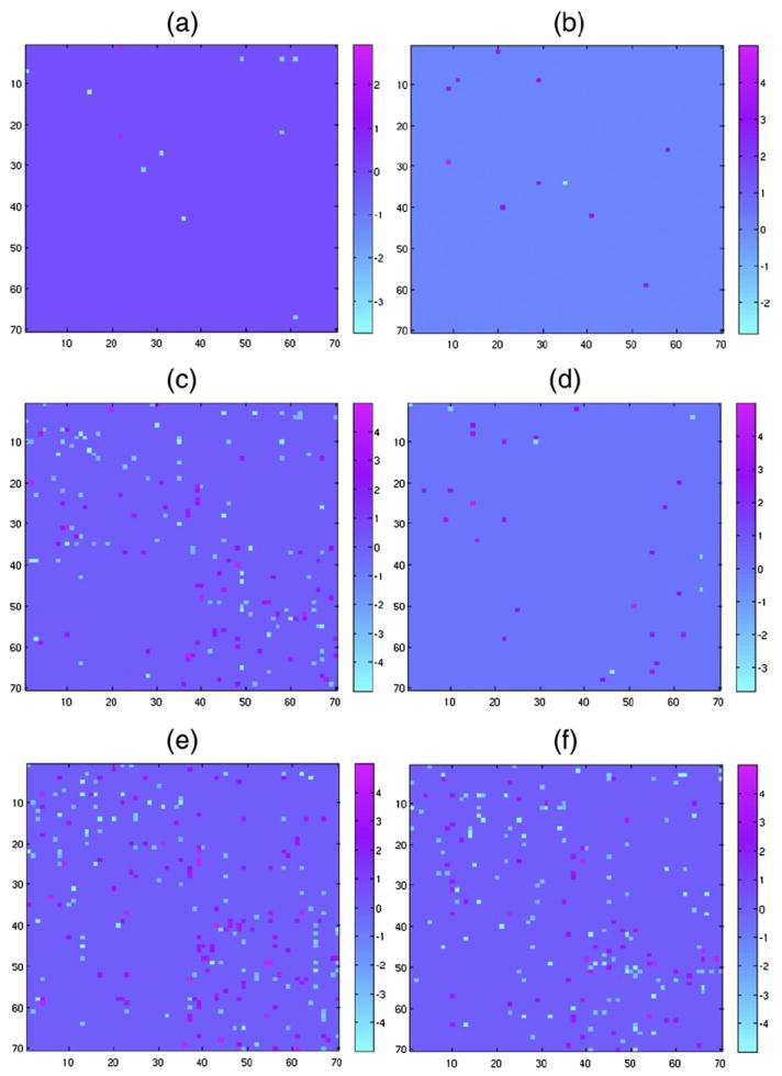
Z-score Kinship differences using the connectivity matrix. a) Identical twins vs non-identical multiples, b) identical twins vs siblings, c) identical twins vs unrelated, d) non-identical multiples vs siblings, e) non-identical multiples vs unrelated, and f) siblings vs unrelated. The color map indicates where the differences are higher for the first group (magenta) or for the second (cyan).
Of special interest are the connections that show the highest Z-score differences between identical twins and non-identical twins (Fig. 5): Lateral Orbitofrontal–Middle Temporal, Rostral middle frontal–Supra-marginal, and Supra–marginal–Rostral middle frontal, in the left hemisphere, and the inter-hemispheric connection Corpus callosum (left)–Medial Orbitofrontal (right). Most of the differentiating connections between identical twins and non-identical twins are either in the left hemisphere or in the inter-hemispheric connections. A similar behavior can be observed on the differences between identical twins and nontwin siblings.
Topological metrics
We now concentrate on the topological metrics and study their strength in distinguishing between the different groups and between real brain networks and random ones.
Random networks
We first report differences between real brain connectivity networks and random networks, obtained by rewiring, at random, the original brain connectivity networks while preserving the in and out node degrees (recall that following the normalization, the obtained networks are directed). Table 6 shows the mean and standard deviation (within parenthesis) of the topological metrics tested, and the Z-score for the difference between the real networks and the corresponding random networks for each topological metric.
Table 6.
Global topological metrics comparing brain connectivity with random networks.
| Metric | Human brain | Random | Z-score |
|---|---|---|---|
| γ | 2.84 (1.44) | – | – |
| Clustering coefficient | 0.0766 (0.0130) | 0.0148 (0.0019) | 13.6 |
| Characteristic path | 77.50 (18.9) | 77.5 (18.9) | 0 |
| Node betweenness | 155.17 (12) | 147.64 (8.72) | 0.51 |
| Modularity | 0.7029 (0.0195) | 0.3380 (0.0187) | 13.51 |
| Rentian scale | 0.6958 (0.0394) | 0.7957 (0.031) | 2.0 |
| PageRank | 0.0143 (0.0096) | 0.0143 (0.084) | 0 |
| Estrada index | 73.1 (0.87) | 71.78 (0.55) | 1.28 |
| Triangular motif 9 | 3.8680 (0.7077) | 0.589 (0.173) | 4.50 |
| Triangular motif 13 | 1.8591 (0.4685) | 0.042 (0.0253) | 3.87 |
The exponent γ of the scale-free, node degree truncated power law distribution (Boccaletti et al., 2006; Bullmore and Bassett, 2011), is also shown. From the 13 possible directed motifs of size three mentioned before (Fig. S2), only motifs 9 and 13 are present in the brain connectivity matrices analyzed here, and therefore only the intensity (Global and node levels section) of these two motifs are compared in the table.
The FDR multiple hypothesis testing error control rejects all null hypothesis with a Z-score equal or above 2.12, at a family-wise error control level of 0.05. Hence, the global clustering coefficient, modularity, and motifs 9 and 13, can be used to differentiate real brain connectivity networks from their corresponding random network.
As the nodes’ degree in the brain connectivity networks follows a truncated power law, we can say that these networks are scale-free.
Since the characteristic path of these networks is as efficient as that of the corresponding random networks, while the clustering coefficient and modularity are higher, we can infer that brain networks satisfy the small-world property, i.e., they combine high modularity with a robust number of inter-modular short paths (Boccaletti et al., 2006; Rubinov and Sporns, 2010).
We have then demonstrated small-worldness of anatomical brain connectivity networks using a relatively large number of samples, and found that, according to other topological metrics, the networks are non-random.
Sex differences
Following the hierarchical scheme of Multiple families of hypothesis testing section (see also Fig. 1), we threshold the connectivity matrices at different screening values and compute the one-tailed p-values obtained from the bootstrapped distributions of the mean (Eq. (15)), for each one of the 9 topological metrics considered. Fig. S4 details these results in terms of the Z-score for each topological metric, when the connectivity matrices are thresholded in the [0, 0.05] range, as well as the BH-FDR threshold. The BH-FDR method requires a minimum Z-score of 2.5, from which we conclude that only the clustering coefficient satisfies the FDR error control at the node level. In addition, the eigenvalues of the communicability matrix may be tested for statistical significance at this level (Fig. 1), to check if the communicability matrix should be tested at the node-to-node level.
Fig. 6a shows the Z-score for the differences in the clustering coefficient, due to sex, on each node; while Fig. 6b shows the Z-score for the eigenvalue differences of the communicability matrix, also due to sex. Higher clustering coefficients for women are shown in magenta, while higher clustering coefficients in men are indicated in cyan. Figs. 6a and b also indicate, in black dashed lines, the minimum Zscore (2.13) required by the BH-FDR error control on both families of tests, at q=0.05. Table S14 in the supplement details the sex differences in the clustering coefficient. In this figure, most differences are in the left hemisphere, which agrees with previous results indicating women have a higher brain connectivity than men in the left hemisphere (Gong et al., 2009; Jahanshad et al., 2011). Here, we obtained similar results with a relatively larger number of HARDI images and using all the brain regions indicated in Table S1.
Fig. 6.

Sex differences considering a) the clustering coefficient, b) the communicability eigenvalues.
We found that the following cortical regions in the left hemisphere have a larger clustering coefficient in women than in men: Caudal Anterior Cingulate, Pars Orbitalis, Rostral Anterior Cingulate, Rostral Middle Frontal. In the right hemisphere, we found that the Cuneus and Middle Temporal cortical regions have also a larger clustering coefficient in women than inmen.
Fig. 6b indicates that in the spectral decomposition of the communicability matrix (Node-to-node level section), one eigenvalue was found to be statistically significant for the differences between women (magenta) and men (cyan), so there are sex differences in the communicability matrix at the node-to-node level.
Figs. 7a and b show the Z-score for the statistically significant sex differences in the edge betweenness centrality (EBC) and the communicability matrix, respectively, due to sex. For simplicity, the figures only show the Z-scores for the sex differences exceeding the minimum Z-score (3.29) required by the BH-FDR error control over both families of hypothesis tests at the 0.05 level. In both figures, higher EBC or communicability values for women are indicated in magenta, while higher EBC or communicability values for men are indicated in cyan.
Fig. 7.
Sex differences considering a) the edge betweenness centrality, b) the communicability matrix.
As seen in Fig. 7a, only five entries in the EBC matrix are statistically significant at this confidence level, and are indicated in more detail in Table S15 (Supplementary material). In particular, the EBC metric is higher in women than in men for the following connections in the left hemisphere: Non-cortical–Lingual and Lingual–Parahippocampal. In the right hemisphere, we found that the EBC metric is higher in women than in men for the Precuneus–Corpus Callosum connection. Finally, the EBC metric on the inter-hemispheric connection Supra-marginal (left)–Peri-calcarine (right) is also higher in women than in men. The p-values are around 10−4, indicating a very high confidence level.
Fig. 7b shows that 12 differences in the directed communicability matrix are statistically significant. These differences are explained in more detail in Table S16 (supplementary material). In general, women have higher directed communicability values, in the inter-hemispheric region, than men. These communicability values are very small (3×10⁻⁸ to 7×10⁻⁴); this is because only long walks are present between the indicated nodes, and the contribution of those walks to the communicability matrix are significantly reduced by the factorial of the walk length on Eq. (15). For subsequent studies that focus on the communicability matrix, we recommend zooming in on longer walks, as suggested in Estrada (2010).
Most of the statistically significant differences found between women and men in the communicability matrix are in the interhemispheric region and the p-values of these differences are of the order of 10−4. In particular, the highest differences found were Middle Temporal (left)–Medial Orbitofrontal (right), Frontal pole (right)–Parahippocampal (left), Superior Temporal (left)–Medial Orbitofrontal (right), Transverse temporal (right)–Parahippocampal (left), and Lingual (right)–Parahippocampal (left).
Finally, the overall FDR for this line of research is FDR ≤3q=0.15 (see Topological metrics section).
Kinship differences
As in the previous section, we thresholded the connectivity matrices at different screening values and compute the one-tailed p-values obtained from the bootstrapped distributions of the mean (Eq. (15)), for each one of the 9 topological metrics considered and for all pair-wise comparisons of kinship groups. The BH-FDR method requires a minimum Z-score in the 2.8–3.0 range, depending on the threshold used (Fig. S5 shows these results in greater detail). None of the global topologicalmetricswas statistically significant, when controlling the false discoveries at the 0.05 or even at the 0.1 level. This is likely because there are 9×6=54 hypothesis tests for all possible pair-wise comparisons of kinship. ANOVA single factor F-ratio reduces this number to 34 on average, but still there are too many comparisons and most global metrics have very low Z-scores (high p-values). One possibility for future analysis would be to consider each case independently, providing different metrics for each pair-wise comparison. However, we decided to follow the hierarchical screening process (see Fig. 1), and test only the communicability matrix eigenvalues at the node level.
Fig. 8 shows the communicability eigenvalues for all possible pairwise comparisons. The communicability eigenvalues do not provide differentiation between identical twins and unrelated pairs of individuals at the minimum Z-score (2.12) required by the BH-FDR error control. This indicates that the communicability matrix might not be able to distinguish kinship relationships at the node-to-node level. The fact that the eigenvalues of the communicability matrix could not distinguish all kinship pair-wise comparisons does not necessarily imply that we cannot find differences using the communicability matrix. However, as explained in Multiple families of hypothesis testing section, we follow a conservative approach, and do not test the communicability matrix at the highest resolution. A complementary study focusing just on the communicability matrix could test it directly to see if it provides statistically significant differences in kinship.
Fig. 8.

Z-score kinship differences considering the communicability eigenvalues: a) Identical twins vs non-identical multiples, b) identical twins vs siblings, c) identical twins vs unrelated, d) non-identical multiples vs siblings, e) non-identical multiples vs unrelated, and f) siblings vs unrelated.
Fig. 9 shows the statistically significant edge betweenness centrality (EBC) differences for all pair-wise kinship comparisons. The EBC matrix does provide significant differences for kinship identification at the required BH-FDR error control (Z-score above 2.87). In particular, the connections that show the highest Z-score differences between identical twins and non-identical twins were (Fig. 9): Superior Frontal (right)–Caudal Anterior Cingulate (left), Middle temporal (right)–Parahippocampal (right), Precuneus (left)–Precuneus (right), Corpus Callosum (right)–Rostral Middle Frontal (right), and Parahippocampal (left)–Middle temporal (left).
Fig. 9.

Z-score kinship differences considering edge betweenness centrality: a) Identical twins vs non-identical multiples, b) identical twins vs siblings, c) identical twins vs unrelated, d) non-identical multiples vs siblings, e) non-identical multiples vs unrelated, and f) siblings vs unrelated.
The overall FDR for this line of research is FDR ≤3q=0.15 (see Topological metrics section).
Discussion
Normalization
In Computing connectivity matrices and brain networks section, we chose a normalization (Eq. (3)) that aims to reduce cortical volume differences (caused by brain size differences for instance). It would be very interesting to study how this normalization affects the results if there are global differences in brain size between groups. In a degenerative disease such as Alzheimer’s disease, for example, there is interest in whether network measures of brain connectivity are altered by the disease. If they are, it is incumbent on those analyzing the data to find out if the network differences are reducible to a simpler effect, such as the absolute or relative size of a cortical region becoming smaller. In Alzheimer’s disease and mild cognitive impairment, for example, we know that there is disproportionate atrophy in the temporal, entorhinal, and cingulate cortices (Apostolova and Thompson, 2008; Thompson et al., 2003), and so any changes in the counts and density of fibers innervating those areas should be tested to see if the changes are due to volume differences in the cortical projection areas. If the proportion of fibers connecting a given cortical region to the other cortical regions remains the same in an atrophic brain relative to a healthy brain, then the network properties of connectivity would not differ after such a normalization. However, if we do normalize the connectivity matrices for the sizes in the cortical regions, it would be possible to infer if the disease affects connectivity above and beyond what would be expected from the size of the cortical regions alone. Alzheimer’s disease is thought to preferentially impair temporal and limbic connectivity, at least early in the disease, and it is interesting to know if the level of cortical disconnection goes beyond what would be seen in a normal person with smaller cortical subregions in these areas. Normalization of network measures to cortical ROI size can achieve this. Most neurodegenerative diseases are expected to influence some connections more than others, generating a change in the proportion of fibers dedicated to each connection, when compared to the same cortical region and corresponding connections on a healthy brain. The overall network analysis framework here developed is currently under investigation for such studies, such as neurodenegeration in HIV where basal ganglia, motor and frontal circuits tend to be more greatly impaired than others (Thompson et al., 2005).
Classification using machine learning methods
Best overall classification performance was obtained using the normalization indicated by Eq. (3) (Estimation of brain structural connectivity and Classification sections). With this normalization, we classified brain connectivity networks, according to sex and kinship classes, with high accuracy, based on the raw connectivity matrices and their associated topological metrics, mainly at the node-to-node level. In particular, the edge betweenness and the generalized communicability matrix were powerful for this task. These results should extend well to unobserved data, as evaluated by the formal 10-fold cross-validation and permutation tests. On the other hand, sex and kinship classification results were weak using topological metrics at the node level. This makes sense due to the large variability of the connectivity matrices that live in a very high dimensional space (ℝn2, n = 70), requiring a higher number of features at the node-to-node resolution.
We cannot numerically compare our sex and kinship machine learning based classification results with previous work, since to the best of our knowledge, no previous work has performed such studies, starting from the raw connectivity matrices or associated topological metrics.15
A key advantage in achieving the classification results reported here was provided by the embedded SVM-based automatic feature selection algorithm (Classification section). This feature selection algorithm evaluates subgroups of features, eliminating redundancies and identifying features, that when considered individually might not be very influential, but can be so as a group. The number of features selected by this feature selection method is close to (but lower than) the number of samples. This hints that each connectivity matrix provides distinctive features, unobtainable from the remaining ones. Therefore, it will be interesting to investigate, as we increase the number of samples, where the number of features increases to a point where it saturates.
Of interest, also, would be to compare ranking versus wrappers feature selection methods; in combination with different classifiers such as logistic, Bayesian, neural networks. A larger study should be conducted to test these classifiers on different datasets and with different tractography algorithms (see Dependence on the tractography algorithm section for a discussion).
Hypothesis testing
Sex differences
We found significant statistical differences, due to sex, in the mean values of 36 edges in the connectivity matrices. In line with prior work, we found that there are, on average, structural brain connectivity differences between women and men. In particular, women have higher probability of inter-hemispheric connections than men, as well as higher probabilities of connections on both hemispheres (as defined in Estimation of brain structural connectivity section), with some exceptions of course (Fig. 4). This seems to suggest that on average, women have great structural connectivity supporting interhemispheric communication than men. The higher strength of the connections in both hemispheres seems to suggest that the communication between the cortical regions associated with those connections is slightly better supported structurally in women than in men.
We must point out here however that these differences are on average. Given the large variability of brain connectivity networks, we can always find individual men with higher connectivity values than some women, e.g., for the features indicated in Fig. 4 (and Table S10).
We also found here that the topological metrics mean clustering coefficient, communicability matrix, and edge betweenness centrality, allow us to distinguish between men and women. In particular, the mean clustering coefficient is higher in women than in men, especially in the left hemisphere and in the cortical regions indicated in Topological metrics section. On average, the neighborhood of these cortical regions is more strongly connected for women than for men. We also find that women have a statistically significant higher edge betweenness centrality metric in five connections (Topological metrics section). This means that these connections are more frequently used on shortest path communications in women than in men. Finally, we found that women have also statistically significant higher communicability values centered on the inter-hemispheric connections indicated in Topological metrics section. This suggest that the inter-hemispheric communication is stronger in women than in men, supporting the results from the connectivity matrices, but now at a higher scale that includes walks of any length.
Previous results on structural differences in the brain connectivity matrix (Jahanshad et al., 2011) and some topological metrics (different from the ones used here), on the associated graph (Gong et al., 2009), agree with the results of this work. In particular, these studies indicate that women have stronger inter-hemispheric connections than men (Jahanshad et al., 2011), that women show greater overall cortical connectivity, and that the underlying organization of their cortical networks is more efficient, both locally and globally (Gong et al., 2009), all in agreement with our results. We arrived here at the same overall conclusions using a larger number of high quality HARDI images, a larger number of topological metrics, and formal control of the overall FDR.
Kinship differences
We found significant statistical differences in the mean distribution of the pair-wise absolute differences in the connectivity matrices and associated topological metrics, allowing us to distinguish among the kinship classes of identical twins, nonidentical twins, non-twin siblings, and unrelated pairs of individuals. As expected from a genetically influenced trait, these differences increase as the pair of subjects is less and less related. For instance, the structural differences between identical twins and non-identical twins are less than the structural differences between twins and non-twin siblings. We cannot make the same kind of comparisons we did between females and males, since the differences reported correspond to differences among classes, where each class is constituted by within-class pairwise differences. The differences reported here were made explicitly for classification purposes, using machine learning methods and hypothesis testing.
Previous and complementary studies on structural brain connectivity differences due to inheritance (Jahanshad et al., 2010; Thompson et al., 2001) cannot be directly compared with our results, since those studies do not work directly with the raw connectivity matrices.
Overall the sex and kinship classification performances (with automatic feature selection) are very good using the communicability and edge betweenness topological metrics, but slightly inferior to using the connectivity matrices directly. We believe that the reason for this is that topological metrics are at a higher scale and offer less detail than edges.
Dependence on the tractography algorithm
A key issue in the repeatability of the findings of any study on structural brain differences based on the DWI-derived connectivity matrix, is the (possible) strong dependence on the tractography algorithm, and the parameters used for such algorithm. Indeed, this study, as well as previous studies on structural brain connectivity, assumes that the number of pathways connecting any pair of cortical regions has been correctly identified by tractography. Nevertheless, tractography results can vary significantly depending on the algorithm and its parameters, the signal to noise ratio of the data, and registration (see for instance Hagmann et al., 2006; Shimony et al., 2006). In particular, simple tensor-based tractography algorithms produce quite different results from ODF-based models (Hagmann et al., 2006), and even the most sophisticated tractography algorithms can produce different results when different parameters are employed.
Taking into account this caveat, we used a state-of-the-art probabilistic HARDI tractography algorithm (Estimation of brain structural connectivity section), performing an exhaustive search of all the possible anatomical connections, avoiding thus local minima, and hence being robust to the variability with respect to different parameters. The results presented here, as well as previous similar studies, are subject to the (unknown) accuracy of the tractography algorithm, and thus statistical results may vary.
In order to further increase the confidence on our results, in addition to the ODF-based probabilistic tractography algorithm used here, we tested a simpler, less robust but very popular tensor-based tractography algorithm implemented in the Trackvis toolbox.16 We do not report in detail the results from this tractography, since in general probabilistic tractography algorithms are superior (Hagmann et al., 2006), and in particular the one used here (Aganj et al., 2010). Nevertheless, we now briefly discuss how the results using this tensorbased tractography model compare with the detailed results reported in Results section. Selected snapshots of the results with this tractography are presented in the supplementary material, Figs. S6–S8.
Overall, the classification accuracies are similar using both tractography models. In addition, the overall sex differences are qualitatively the same: higher inter-hemispheric and overall within hemisphere connections in females than in males. We also obtained statistically significant features to discriminate all the kinship classes using the same topological metrics indicated before. However, the particular features identified as significant for classification, and using hypothesis testing, are different for both tractography algorithms. This is clearly not a failure of the methodology proposed here, but a limitation of the current state-of-the-art tractography algorithms. Moreover, the lower robustness of the tensor-based tractography algorithms is expected to lead to such difference in selected features, since for example, certain less-complex pathways can be more consistent and less affected by such lower tractography performance. Features selected by ODF-based probabilistic tractography are expected to be more reliable.
While the methodology here proposed is expected to be robust to small variations in the connectivity matrices, it can certainly be affected by artifacts coming from tractography or other sources that could seriously bias the connectivity matrices. The robustness of the proposed method relies in turn on the robustness of the feature selection, classification, performance evaluation, and FDR error control methods, that as shown in the Methods, have strong theoretical and practical foundations.
FDR error control
There is a general consensus in the scientific community that the FDR must be controlled when multiple hypotheses are being tested on the same data. There is however no general agreement on how to control the FDR when multiple families of hypotheses are tested along the same line of research. As shown in Hypothesis testing section, a strict FDR error control on multiple families of hypotheses can significantly reduce the number of null-hypotheses that are rejected, hence, the making of more discoveries.
This is an issue that has been seriously addressed recently, especially in gene expression studies, where multiple families of thousands of hypotheses must be tested on each gene (Yekutieli, 2008). We combined the screening method proposed by Rubinov and Sporns (2010), Bullmore and Bassett (2011), Achard and Bullmore (2007), Bassett et al. (2008), and the ANOVA F-ratio test, to reduce the number of uninteresting null-hypotheses, with the novel hierarchical approach of Yekutieli (2008), Benjamini and Yekutieli (2005), Yekutieli et al. (2006), to control the FDR, increasing thus the statistical power when compared to a naive overall FDR error control. In spite of this, we cannot reject any null-hypothesis on the kinship classes, at the topological global level, and only one of the hypotheses tested at this level was significant for sex differences. We could have dropped the control of the overall FDR error considering that is was too strict, but did not, because that undermines the essence of the FDR error control. Indeed, the same reason why we must control the false discovery rate on single families of hypotheses testing, subsists on multiple families of hypotheses testing (on the same research line): the higher the number of hypotheses being tested on the same data, the higher the probability of rejecting nullhypotheses by chance, especially, when most of the null-hypotheses are true or can barely be rejected either individually or at the family level.
There is however a need for less conservative FDR error control, especially when the expected proportion of true null-hypotheses is high, i.e., we expect few true discoveries among many true nullhypotheses. The high number of individuals considered here improves the accuracy of the estimated distribution of the mean (via bootstrapping). However, the FDR error control is blind to this, since the number of hypotheses being tested depends only on the number of features at each scale (see Methods), which, in our case, can be O(n2), n being the number of nodes in the network. The FDR error control penalizes all the same smaller and larger studies. Further studies should be conducted to make the FDR error control less conservative, especially, on larger population studies.
Conclusion
In this large scale HARDI study of 303 individuals, we introduced a unifying, robust and general method to investigate brain connectivity differences among individuals (including pairs of individuals) using machine learning and hypothesis testing methods. We also reported differences among groups or classes of individuals using multiple hypotheses tests at several levels of data hierarchy.
We considered both: raw connectivity matrices and derived topological metrics, at multiple levels: global, single node, and node-to-node. Feature selection using a wrapper (or embedded method) was critical to eliminate, for classification purposes, uninformative connections in the connectivity matrix or topological metrics on the associated digraphs.
Future work will focus on metrics at different scales and at the highest resolution scale (as was done with the connectivity matrices). The study will also be extended to larger datasets, permitting other kinds of genetic studies, and to denser connectivity matrices derived from various tractography methods. Of great interest is a formal study of the sensitivity of classification, feature selection, and multiple hypotheses testing to the tractography model.
Supplementary Material
Acknowledgments
Work partially supported by NIH P41 RR008079, NIH P30 NS057091, NIH R01 EB008432, ONR, NGA, NSF, NSSEFF/AFOSR, and ARO. NJ was additionally supported by NIH NLM Grant T15 LM07356. This study was supported by grant number RO1 HD050735 from the National Institute of Child Health and Human Development, USA, and Project Grant 496682 from the National Health and Medical Research Council, Australia. Additional support for algorithm development was provided by the NIA, NIBIB, and the National Center for Research Resources (AG016570, EB01651, RR019771 to PT). The authors would like to thank the feedback provided by Dr. Daniel Yekutieli in the correct interpretation of the hierarchical control of the FDR and also Dr. Ernesto Estrada for his feedback on the correct interpretation of the communicability matrix for directed graphs, and for providing us with further bibliography in the subject. We are also grateful to the twins for their willingness to participate in our studies, and research nurses, Marlene Grace and Ann Eldridge, Queensland Institute of Medical Research, for twin recruitment.
Appendix A
Additional implementation details
We used the publicly available implementations of topological metrics in the Brain Connectivity Toolbox (BCT),17 that works with weighted directed graphs. Newer metrics such as the PageRank and centrality and communicability measures, based on subgraphs, are not available in the BCT toolbox. Nevertheless, a free implementation of the PageRank can be found on the web,18 and Ernesto’s centrality and communicability measures can be easily obtained using the new matrix exponential function (expm) in Matlab.19
In this work, we use the Waikato Environment for Knowledge Analysis (weka) data mining software,20 which provides feature selection, classification, regression and n-fold cross-validation tools.21 Permutation tests were implemented in JAVA using the weka, libsvm,22 and Java Statistical Classes23 (jsc) libraries. The permutation tests consist on training the classifier with the selected features and 10-fold cross-validation, over 1000 random permutations of the dataset labels, in order to generate the null-hypothesis distribution. Since, the computed p-values of the permutation tests strongly depends on the performance of the classification being tested (Ojala and Garriga, 2010), we used the average of the classification performance over 1000 different random splittings of the dataset.24 In addition, the classification performance is not evaluated using a single parameter. We used here overall classification accuracy, Balanced Error Rate (BER)25 area under the Receiver Operating Characteristic (ROC), kappa statistic, and confusion matrices.
In general, classifier performance can be biased due to large differences in the number of samples for each class. The weka toolbox allows the use of a weight to compensate for the differences in the number of samples. Nevertheless, this weight did not produce significant classification differences as compared to the unweighted samples, as SVMs are less dependent on sample size, because they rely on a few support vectors.
Single effects F-ratio
Here, we will refer to populations, factors and treatments as it is usual in experimental design. The population here refers to the bootstrapped mean differences, due to sex for instance. Factors refer here to sex differences measured by each one of the topological metrics considered (Topological metrics section, Fig. 1), while treatments refer to the differences on each node or node to node that produce differences in the mean value of the topological metric at those scales. For instance, a factor is the clustering difference (measured by the clustering coefficient) due to sex, while the treatments correspond to the clustering differences on each node that lead to differences in the clustering coefficient on each node. Here, we use single factor ANOVA F-ratios to screen out treatments that are not statistically significant.
The single effects F-ratio is computed as the ratio of the mean square treatment (main) effect and the mean square (variance within) treatment error (Winer, 1971),
where dij are the observed differences at the ith node or node to node i=1,…,n and jth bootstrapped sample j=1,…,B, d̄i. the mean value of the bootstrapped samples at i, and d̄.., the overall population mean. Now, F-ratios where Fi≥F(q, 1, B − 1), being F the F-distribution, are considered statistically significant at the error control level q.
The usual ANOVA F-ratios divide main effects by the pooled experimental error, assuming that error variances (within treatment variability) are all equal, which is a strong assumption not usually met in practice. The F-ratio used here allows differences in the experimental error on each treatment. This implies that this F-ratio does not follow exactly an F-distribution, however, the sampling distribution of these F-ratios can be approximated by the F-distribution (Winer, 1971). In addition, ANOVA F-ratios also assume independence (no interaction) on each treatment. In general, this independence is not met in our case, since nodes are neighbors of other nodes. For instance the neighbors of a node with a high clustering coefficient might also have high clustering coefficient, since the neighbors are also in the same cluster. However, we are working here with differences and differences reduce or eliminate these positive interaction effects. Hence, in our case dependence among treatments should be weak. Nevertheless, if there is dependence among treatments, the results of the F-ratio test are optimistic (Winer, 1971), meaning that more treatments are accepted as influential. In our case, it means that the test never rejects a true influential effect, while non-influential treatments will be rejected by the subsequent FDR tests. The only purpose of this screening test is to reduce the number of non-interesting hypotheses to test using FDR error control, and as we have seen here, this test does just that despite its simplicity and assumptions.
The single effects F-ratio screening is performed here controlling the error rate at q=0.15 at the global and node level in order to avoid overly reducing the number of hypotheses to be tested, and a 0.05 level of significance at the node-to-node level, when thousands of hypotheses are present.
Regression analysis
We tested the statistical significance of different linear regression models including the variables sex (coded as −1 men, +1 women), brain volumes,26 age, and different degrees of interactions, in modeling the probability of connection on the whole dataset. We found that the following model has statistical significance modeling the connectivity matrices, on average,
| (17) |
where predictors S,B,A represent sex, brain volume, and age respectively, while SB represents the interaction between sex and brain volume. Given the strong correlation between sex and brain size, we employed ridge regression that provides regularization when there is strong collinearity between predictors. The used Matlab implementation of ridge regression also centers and standardizes the predictors internally, which improves stability and allow for proper comparison of the regression coefficients.
Using the normalization provided by Eq. (3), the regression coefficients were β1=6.15×10⁻³, β2=−1.87×10⁻⁵, β3=−2.12×10⁻⁴, β4=−6.23×10⁻³. Where we can see that the effect of sex is about 328 times larger than that of brain size and about 30 times larger than that of age. However, there is still strong negative interaction due to brain size.
We perform an F-test of significance of the regression model using the un-centered and un-standardized predictors. We found that we can reject the null hypothesis that all regression coefficients in the model are zero, with a level of significance of 0.002. Now, testing the significance of each factor (using standard t-test), we found that the sex and age coefficients are statistically significant with a level of significance of 2.8×10⁻⁴ and 0.048, respectively, but the brain volume coefficient and interaction term are not statistically significant. Given that the effect of age and interaction with brain volume are both negative and much lower than the effect of sex, we disregard those effects in the analysis. The effect of age and brain size (through interaction) causes a reduction in the statistical power of the analysis performed (since their effect is negative), which means that some brain connectivity differences due to sex that might have been influential could not be detected. This is a small price to pay in exchange for simplicity in the analysis and proves the importance of the normalization chosen.
The regression coefficients for the centered and standardized predictors using the normalization provided by Eq. (1) were β1=1.52×10⁻³, β2=7.93×10⁻⁴, β3=2.07×10⁻⁴, β4=−8.9×10⁻³, which means that the sex effect is about 2 times larger than that of brain size, 7 times larger than that of age, and about 2 times the interaction with brain size. Formally, the model is statistically significant, with a significance level of 7.5×10⁻⁴, and the t-test on each factor reveals that the coefficients of brain size and age are statistically significant with a significance level of 1.5×10⁻⁷ and 0.035, respectively, while the sex coefficient is only statistically significant at a significance level of 0.18. This means that the brain volume and age are more significant than sex differences and hence any differences found using this normalization alone (without further processing) could be false.
The regression coefficients for the centered and standardized predictors using the normalization provided by Eq. (2) were β1=7.58×10⁻³, β2=4.49×10⁻⁵, β3=3.7×10⁻⁴, β4=−7.6×10⁻³, which means that the sex effect is about 170 times larger than that of brain size, 20 times larger than that of age, and there is strong interaction with brain size. Formally, the model is statistically significant, with a significance level of 0.05, and the t-test on each factor reveals that the regression coefficients of sex and age are statistically significant with a significance level of 0.007 and 0.046, respectively, while brain size and its interaction with sex are not statistically significant. As can be seen this normalization is almost as good as Eq. (3), butwe preferred Eq. (3), since it is also superior in terms of classification performance (see Classification section) and holds the interpretation described above.
Footnotes
The group of non-twin siblings overlaps the group of twins and triplets, since an individual can have 2 or more siblings that are twins (or triplets).
The expected deformations are only translation, rotation, and anisotropic scaling; no shearing between T1s of the same subject.
In the near future, this algorithm will be released through the Neuroimaging Informatics Tools and Resources Clearinghouse (NITRC) online repository, and is available upon request.
The basic method introduced later for analyzing brain networks, in particular the features for undirected networks and the statistical analysis, can still be applied to the other possible normalizations as well.
Of course, we only look for statistically significant differences where the number of connections detected is more than zero.
PCA for instance is a projection of the original features onto the matrix eigen-space, and hence is a linear combination of the original features.
Training with 90% of the data and testing on the remaining 10%, and repeating the process 10 times with randomly selected training and testing samples.
As it is usual in binary classification, we report sensitivity and specificity for women only, given that the sensitivity for men is numerically the same as the specificity for women and the specificity for men is numerically the same as the sensitivity for women.
The Rentian scale does not use actual the weights or the direction information.
Recall that the normalized connectivity matrices are all in the [0, 1] range.
Recall that for the kinship classes, we will be comparing connectivity matrices that represent the absolute connectivity differences within each group, and not the connectivity of each individual or pairs of individuals. Hence, differences between two kinship classes refer here to differences between the two means of the within-group differences.
Notice in Tables S3–S4 that EBC has a slightly higher classification than communicability, but it has a higher BER error, hence we choose here the generalized communicability matrix.
Of course, other studies focusing on sex and inheritance differences have been conducted in the past, as mentioned in the text and cited in the bibliography.
http://read.pudn.com/downloads149/sourcecode/math/642925/pagerank.m__.htm or http://www.levmuchnik.net/Content/Networks/NetworkPackageReference.html#Algorithms.
Alternatively, the rapidMiner package provides multithreading and more flexibility than weka, at the expense of a steeper learning curve.
This is achieved in weka by changing at random the seed.
Chosen in the NIPS 2003 feature selection challenge as the main judging criterion.
The brain volume was calculated from the manually skull-stripped images in mm3 and then converted to liters.
Appendix B. Supplementary Data
Supplementary data to this article can be found online at doi:10. 1016/j.neuroimage.2011.10.096.
Contributor Information
Julio M. Duarte-Carvajalino, Email: duart022@umn.edu.
Neda Jahanshad, Email: neda.jahanshad@loni.ucla.edu.
Christophe Lenglet, Email: clenglet@umn.edu.
Katie L. McMahon, Email: katie.mcmahon@cai.uq.edu.au.
Greig I. de Zubicaray, Email: greig.dezubicaray@uq.edu.au.
Nicholas G. Martin, Email: Nick.Martin@qimr.edu.au.
Margaret J. Wright, Email: Margie.Wright@qimr.edu.au.
Paul M. Thompson, Email: thompson@loni.ucla.edu.
Guillermo Sapiro, Email: guille@umn.edu.
References
- Abramovich F, Benjamini Y. Adaptive thresholding of wavelet coefficients. Comput Stat Data Anal. 1996;22:351–361. [Google Scholar]
- Achard S, Bullmore ET. Efficiency and cost of economical brain functional networks. PLoS Comput Biol. 2007;3:e17. doi: 10.1371/journal.pcbi.0030017. [DOI] [PMC free article] [PubMed] [Google Scholar]
- Aganj I, Lenglet C, Sapiro G, Yacoub E, Ugurbil K, Harel N. Reconstruction of the orientation distribution function in single- and multiple-shell q-ball imaging within constant solid angle. Magn Reson Med. 2010;64(2):554–566. doi: 10.1002/mrm.22365. [DOI] [PMC free article] [PubMed] [Google Scholar]
- Amaldi E, Kann V. On the approximation of minimizing non zero variables or unsatisfied relations in linear systems. Theor Comput Sci. 1998;209:237–260. [Google Scholar]
- Apostolova L, Thompson PM. Mapping progressive brain structural changes in early Alzheimer’s disease and mild cognitive impairment. Neuropsycologia. 2008;46(6):1597–1612. doi: 10.1016/j.neuropsychologia.2007.10.026. [DOI] [PMC free article] [PubMed] [Google Scholar]
- Basser PJ, Pierpaoli C. Microstructural and physiological features of tissues elucidated by quantitative-diffusion-tensor MRI. J Magn Reson. 1996;111(3):209–219. doi: 10.1006/jmrb.1996.0086. [DOI] [PubMed] [Google Scholar]
- Bassett DS, Bullmore ET, Verchinski BA, Mattay VS, Weinberger DR, Meyer-Lindenberg A. Hierarchical organization of human cortical networks in health and schizophrenia. J Neurosci. 2008;28(37):9239–9248. doi: 10.1523/JNEUROSCI.1929-08.2008. [DOI] [PMC free article] [PubMed] [Google Scholar]
- Bassett DS, Greenfield DL, Meyer-Lindenberg A, Weinberger DR, Moore SW, Bullmore ET. Efficient physical embedding of topologically complex information processing networks in brains and computer circuits. PLoS Comput Biol. 2010;6(4):e1000748. doi: 10.1371/journal.pcbi.1000748. [DOI] [PMC free article] [PubMed] [Google Scholar]
- Bassett DS, Brown JA, Deshpande V, Carlson JM, Grafton S. Conserved and variable architecture of human white matter connectivity. Neuroimage. 2011;54(2):1262–1279. doi: 10.1016/j.neuroimage.2010.09.006. [DOI] [PubMed] [Google Scholar]
- Behrens TEJ, Berg HJ, Jbabdi S, Rushworth MFS, Woolrich MW. Probabilistic diffusion tractography with multiple fibre orientations: what can we gain? Neuroimage. 2007;34(1):144–155. doi: 10.1016/j.neuroimage.2006.09.018. [DOI] [PMC free article] [PubMed] [Google Scholar]
- Benjamini Y, Hochberg Y. Controlling the false discovery rate: a practical and powerful approach to multiple testing. J R Stat Soc B Met. 1995;57(1):289–300. [Google Scholar]
- Benjamini Y, Hochberg Y. On the adaptive control of the false discovery rate in multiple testing with independent statistics. J Educ Behav Stat. 2000;25(1):60–83. [Google Scholar]
- Benjamini Y, Yekuteli D. The control of the false discovery rate in multiple testing under dependency. Ann Stat. 2001;29(4):1165–1188. [Google Scholar]
- Benjamini Y, Yekuteli D. False discovery rate-adjusted multiple confidence intervals for selected parameters. J Am Stat Assoc. 2005;100:71–81. [Google Scholar]
- Benjamini Y, Yekutieli D. Quantitative trait loci analysis using the false discovery rate. Genetics. 2005;171(2):783–790. doi: 10.1534/genetics.104.036699. [DOI] [PMC free article] [PubMed] [Google Scholar]
- Benjamini Y, Heller R, Yekutieli D. Selective inference in complex research. Philos Trans R Soc Lond B Biol Sci. 2009;367(1906):4255–4271. doi: 10.1098/rsta.2009.0127. [DOI] [PMC free article] [PubMed] [Google Scholar]
- Blondel V, Guillaume J, Lambiotte R, Lefebvre E. Fast unfolding of communities in large networks. J Stat Mech. 2008:1008. [Google Scholar]
- Boccaletti S, Latorab V, Moreno Y, Chavez M, Hwanga D-U. Complex networks: structure and dynamics. Phys Rep. 2006;424(4–5):175–308. [Google Scholar]
- Brin S, Page L. Proc Intl Conf World Wide Web. Vol. 30. Publishers, E.S; 1998. The anatomy of a large-scale hypertextual web search engine; pp. 1–7. [Google Scholar]
- Bullmore ET, Bassett DS. Brain graphs: graphical models of the human brain connectome. Annu Rev Clin Psychol. 2011;7:113–140. doi: 10.1146/annurev-clinpsy-040510-143934. [DOI] [PubMed] [Google Scholar]
- Bullmore ET, Sporns O. Complex brain networks: graph theoretical analysis of structural and functional systems. Nat Rev Neurosci. 2009;10(3):186–198. doi: 10.1038/nrn2575. [DOI] [PubMed] [Google Scholar]
- Crofts JJ, Higham DJ. A weighted communicability measure applied to complex brain networks. J R Soc Interface. 2009;6(33):411–414. doi: 10.1098/rsif.2008.0484. [DOI] [PMC free article] [PubMed] [Google Scholar]
- Davison R, MacKinnon JG. Econometric Theory. Vol. 15. Cambridge University Press; 1999. The size distortion of bootstrap tests. [Google Scholar]
- de Boer R, Schaap M, van der Lijn F, Vrooman HA, de Groot M, van der Lugt A, Ikram MA, Vernooij MW, Breteler MM, Niessen WJ. Statistical analysis ofminimum cost path based structural brain connectivity. Neuroimage. 2011;55(2):557–565. doi: 10.1016/j.neuroimage.2010.12.012. [DOI] [PubMed] [Google Scholar]
- Dosenbach NUF, Nardos B, Cohen AL, Fair DA, Power JD, Church JA, Nelson SM, Wig GS, Vogel AC, Lessov-Schlaggar CN, Barnes KA, Dubis JW, Feczko E, Coalson RS, Pruett JR, Barch DM, Petersen SE, Schlaggar BL. Prediction of individual brain maturity using fMRI. Science. 2010;329(5997):1358–1361. doi: 10.1126/science.1194144. [DOI] [PMC free article] [PubMed] [Google Scholar]
- Duda RO, Hart PE. Use of the Hough transformation to detect lines and curves in pictures. Commun ACM. 1972;15(1) [Google Scholar]
- Easley D, Kleinberg J. Networks, Crowds, and Markets: Reasoning about a Highly Connected World. Cambridge University Press; 2010. [Google Scholar]
- Estrada E. Generalized walks-based centrality measures for complex biological networks. J Theor Biol. 2010;263(4):556–565. doi: 10.1016/j.jtbi.2010.01.014. [DOI] [PubMed] [Google Scholar]
- Estrada E, Higham DJ. Network properties revealed through matrix functions. SIAM Rev. 2010;52(4):696–714. [Google Scholar]
- Fischl B, van der Kouwe A, Destrieux C, Halgren E, Ségonne F, Salat DH, Busa E, Seidman LJ, Goldstein J, Kennedy D, Caviness V, Makris N, Rosen B, Anders M, Dale AM. Automatically parcellating the human cerebral cortex. Cereb Cortex. 2004;14(1):11–22. doi: 10.1093/cercor/bhg087. [DOI] [PubMed] [Google Scholar]
- Fisher H. From Classical to Modern Probability Theory. 1. Springer; 2011. A History of the Central Limit Theorem. [Google Scholar]
- Fornito A, Zalesky A, Bassett DS, Meunier D, Ellison-Wright I, Yu M, Wood SJ, Shaw K, O’Connor J, Nertney D, Mowry BJ, Pantelis C, Bullmore ET. Genetic influences on cost-efficient organization of human cortical functional networks. J Neurosci. 2011;31(9):3261–3270. doi: 10.1523/JNEUROSCI.4858-10.2011. [DOI] [PMC free article] [PubMed] [Google Scholar]
- Gigandet X, Hagmann P, Kurant M, Cammoun L, Meuli R, Thiran J-P. Estimating the confidence level of white matter connections obtained with MRI tractography. PLoS One. 2008;3(12):e4006. doi: 10.1371/journal.pone.0004006. [DOI] [PMC free article] [PubMed] [Google Scholar]
- Gong G, Rosa-Neto P, Carbonell F, Chen ZJ, He Y, Evans AC. Age- and gender-related differences in the cortical age- and gender-related differences in the cortical anatomical network. J Neurosci. 2009;29(50):15684–15693. doi: 10.1523/JNEUROSCI.2308-09.2009. [DOI] [PMC free article] [PubMed] [Google Scholar]
- Gonzales RC, Woods RE. Digital Image Processing. 3. Prentice Hall; 2008. [Google Scholar]
- Guyon I, Eliseeff A. An introduction to variable and feature selection. J Mach Learn Res. 2003;3:1157–1182. [Google Scholar]
- Guyon I, Weston J, Barnhill S, Vapnik V. Gene selection for cancer classification using support vector machines. Mach Learn. 2002;46(1–3):389–422. [Google Scholar]
- Hagmann P, Kurant M, Gigandet X, Thiran P, Wedeen VJ, Meuli R, Thiran J-T. Mapping human whole-brain structural networks with diffusion MRI. PLoS One. 2007;2(7):e597. doi: 10.1371/journal.pone.0000597. [DOI] [PMC free article] [PubMed] [Google Scholar]
- Hagmann P, Cammoun L, Gigandet X, Meuli R, Honey CJ, Wedeen VJ, Sporns O. Mapping the structural core of human cerebral cortex. PLoS Biol. 2008;6(7):e159. doi: 10.1371/journal.pbio.0060159. [DOI] [PMC free article] [PubMed] [Google Scholar]
- Hagmann P, Jonasson L, Maeder P, Thiran J-P, Wedeen VJ, Meuli R. Understanding diffusion MR imaging techniques: from scalar diffusion-weighted imaging to diffusion tensor imaging and beyond. Radiographics. 2006 Oct;26:S205–S223. doi: 10.1148/rg.26si065510. [DOI] [PubMed] [Google Scholar]
- Hartmann WM. Lecture Notes in Computer Science. Vol. 3732. Springer; 2006. Dimension reduction vs. variable selection; pp. 931–938. [Google Scholar]
- He Y, Chen ZJ, Evans AC. Small-world anatomical networks in the human brain revealed by cortical thickness from MRI. Cereb Cortex. 2007;17(10):2407–2419. doi: 10.1093/cercor/bhl149. [DOI] [PubMed] [Google Scholar]
- Holmes CJ, Hoge R, Collins L, Woods R, Toga AW, Evans AC. Enhancement of MR images using registration for signal averaging. J Comput Assist Tomogr. 1998;22(2):324–333. doi: 10.1097/00004728-199803000-00032. [DOI] [PubMed] [Google Scholar]
- Iturria-Medina Y, Canales-Rodríguez E, Melie-García L, Valdés-Hernández P, Martínez-Montes E, Alemán-Gómez Y, Sánchez-Bornot JM. Characterizing brain anatomical connections using diffusion weighted MRI and graph theory. Neuroimage. 2007;36(3):645–660. doi: 10.1016/j.neuroimage.2007.02.012. [DOI] [PubMed] [Google Scholar]
- Jahanshad N, Lee AD, Barysheva M, McMahon KL, de Zubicaray GI, Martin NG, Wright MJ, Toga AW, Thompson PM. Genetic influences on brain asymmetry: a DTI study of 374 twins and siblings. Neuroimage. 2010;52(2):455–469. doi: 10.1016/j.neuroimage.2010.04.236. [DOI] [PMC free article] [PubMed] [Google Scholar]
- Jahanshad N, Aganj I, Lenglet C, Joshi A, Jin Y, Barysheva M, McMahon K, de Zubiricaray G, Martin N, Wright M, Toga AW, Sapiro G, Thompson PM. Sex differences in the human connectome: 4-tesla high angular resolution diffusion imaging (HARDI) tractography in 234 young adult twins. Proc IEEE Int Symp Biomed Imaging. 2011 doi: 10.1109/ISBI.2011.5872405. [DOI] [PMC free article] [PubMed] [Google Scholar]
- Jensen DD, Cohen PR. Multiple comparisons in induction algorithms. Mach Learn. 2000;38:309–338. [Google Scholar]
- Kriegeskorte N, Simmons WK, Bellgowan PSF, Bake CI. Circular analysis in systems neuroscience: the dangers of double dipping. Nat Neurosci. 2009;12:535–540. doi: 10.1038/nn.2303. [DOI] [PMC free article] [PubMed] [Google Scholar]
- Leonard CM, Towler S, Welcome S, Halderman LK, Otto R, Eckert MA, Chiarello C. Size matters: cerebral volume influences sex differences in neuroanatomy. Cereb Cortex. 2008;18(12):2920–2931. doi: 10.1093/cercor/bhn052. [DOI] [PMC free article] [PubMed] [Google Scholar]
- Leow A, Huang S-C, Geng A, Becker J, Davis S, Toga AW, Thompson PM. Lecture Notes in Computer Science. Vol. 3565. Springer-Verlag; 2005. Inverse consistent mapping in 3D deformable image registration: its construction and statistical properties; pp. 23–57. [DOI] [PubMed] [Google Scholar]
- Lohmann G, Margulies DS, Horstmann A, Pleger B, Lepsien J, Goldhahn D, Schloegl H, Stumvoll M, Villringer A, Turner R. Eigenvector centrality mapping for analyzing connectivity patterns in fMRI data of the human brain. PLoSOne. 2010;5(4):e10232. doi: 10.1371/journal.pone.0010232. [DOI] [PMC free article] [PubMed] [Google Scholar]
- Ojala M, Garriga GC. Permutation tests for studying classifier performance. J Mach Learn Res. 2010;11:1833–1863. [Google Scholar]
- Onnela JP, Saramäki J, Kertész J, Kaski K. Intensity and coherence of motifs in weighted complex networks. Phys Rev E. 2005;71(6):065103. doi: 10.1103/PhysRevE.71.065103. [DOI] [PubMed] [Google Scholar]
- Refaeilzadeh P, Tang L, Liu H. Encyclopedia of Database Systems. Springer; 2009. Cross validation. [Google Scholar]
- Reiner-Benaim A. FDR control by the BH procedure for two-sided correlated tests with implications to gene expression data analysis. Biom J. 2007;49(1):107–126. doi: 10.1002/bimj.200510313. [DOI] [PubMed] [Google Scholar]
- Reiner-Benaim A, Yekuteli D, Letwin NE, Elmer GI, Lee NH, Kafkafi N, Benjamini Y. Associating quantitative behavioral traits with gene expression in the brain: searching for diamonds in the hay. Bioinformatics. 2007;23(17):2239–2246. doi: 10.1093/bioinformatics/btm300. [DOI] [PubMed] [Google Scholar]
- Richiardi J, Eryilmaz H, Schwartz S, Vuilleumier P, Van De Ville D. Decoding brain states from fMRI connectivity graphs. Neuroimage. 2011;56(2):616–626. doi: 10.1016/j.neuroimage.2010.05.081. [DOI] [PubMed] [Google Scholar]
- Rubinov M, Bassett DS. Emerging evidence of connectomic abnormalities in schizophrenia. Neuroscience. 2011;31(17):6263–6265. doi: 10.1523/JNEUROSCI.0382-11.2011. [DOI] [PMC free article] [PubMed] [Google Scholar]
- Rubinov M, Sporns O. Complex network measures of brain connectivity: uses and interpretations. Neuroimage. 2010;52(3):1059–1069. doi: 10.1016/j.neuroimage.2009.10.003. [DOI] [PubMed] [Google Scholar]
- Shepelyansky DL, Zhirov OV. Towards google matrix of brain. Phys Lett A. 2010;374:3206–3209. [Google Scholar]
- Shimony J, Burton H, Epstein AA, McLaren DG, Sun SW, Snyder AZ. Diffusion tensor imaging reveals white matter reorganization in diffusion tensor imaging reveals white matter reorganization in diffusion tensor imaging reveals white matter reorganization in early blind humans. Cereb Cortex. 2006 Nov;16:1653–1661. doi: 10.1093/cercor/bhj102. [DOI] [PMC free article] [PubMed] [Google Scholar]
- Sporns O, Kotter R. Motifs in brain networks. PLoS Biol. 2004;2:e369. doi: 10.1371/journal.pbio.0020369. [DOI] [PMC free article] [PubMed] [Google Scholar]
- Storey JD. A direct approach to false discovery rates. J R Stat Soc B. 2002;64(3):479–498. [Google Scholar]
- Storey JD, Taylor JE, Siegmund D. Strong control, conservative point estimation and simultaneous conservative consistency of false discovery rates: a unified approach. J R Stat Soc B. 2004;66(1):187–205. [Google Scholar]
- Thomason ME, Dennis EL, Joshi AA, Joshi SH, Dinov ID, Chang C, Henry ML, Johnson RF, Thompson PM, Toga AW, Glover GH, Van Horn JD, Gotlib IH. Resting-state fMRI can reliably map neural networks in children. Neuroimage. 2011;55(1):165–175. doi: 10.1016/j.neuroimage.2010.11.080. [DOI] [PMC free article] [PubMed] [Google Scholar]
- Thompson PM, Cannon TD, Narr KL, van Erp T, Poutanen V-P, Huttunen M, Lonnqvist J, Standertskjold-Nordenstam C-G, Kaprio J, Khaledy M, Dail R, Zoumalan CI, Toga AW. Genetic influences on brain structure. Nat Neurosci. 2001;4(12):1253–1258. doi: 10.1038/nn758. [DOI] [PubMed] [Google Scholar]
- Thompson PM, Hayashi KM, de Zubiricaray G, Janke AL, Rose SE, Semple J, Herman D, Hong MS, Dittmer S, Doddrell DM, Toga AW. Dynamics of gray matter loss in Alzheimer’s disease. J Neurosci. 2003;23(3):994–1005. doi: 10.1523/JNEUROSCI.23-03-00994.2003. [DOI] [PMC free article] [PubMed] [Google Scholar]
- Thompson PM, Dutton RA, Hayashi KM, Toga AW, Lopez OL, Aizenstein HJ, Becker JT. Thinning of the cerebral cortex in HIV/AIDS reflects cd4+ t-lymphocyte decline. Proc Natl Acad Sci U S A. 2005;102:15647–15652. doi: 10.1073/pnas.0502548102. [DOI] [PMC free article] [PubMed] [Google Scholar]
- Tuch DS. Q-ball imaging. Magn Reson Med. 2004 Dec;52:1358–1372. doi: 10.1002/mrm.20279. [DOI] [PubMed] [Google Scholar]
- Vapnik VN. Statistical Learning Theory. Wiley-Interscience; 1998. [Google Scholar]
- Westfall PH, Johnson WO, Utts JM. Bayesian perspective on the Bonferroni adjustment. Biometrika. 1997;84(2):419–427. [Google Scholar]
- Winer BJ. Statistical Principles in Experimental Design. 2. Mc Graw-Hill, Inc; 1971. [Google Scholar]
- Yekutieli D. Hierarchical false discovery rate controlling methodology. J Am Stat Assoc. 2008;103(481):309–316. [Google Scholar]
- Yekutieli D, Reiner-Benaim A, Benjamini Y, Elmer GI, Kafkafi N, Letwin NE, Lee NH. Approaches to multiplicity issues in complex research in microarray analysis. Stat Neerl. 2006;60(4):414–437. [Google Scholar]
Associated Data
This section collects any data citations, data availability statements, or supplementary materials included in this article.