Misuse of the linear mixed model when evaluating risk factors of cognitive decline

Abstract

The linear mixed model (LMM), routinely used to describe change over time of outcomes and association with risk factors, assumes that a unit change in any predictor is associated with a constant change in the outcome. When used on psychometric tests, this assumption may not hold. Indeed, psychometric tests usually suffer from ceiling and/or floor effects, and curvilinearity (i.e. varying sensitivity to change).

This work aimed at determining the consequences of such a misspecification when evaluating predictors of cognitive decline. As an alternative to the LMM, two mixed models based on latent processes that handle discrete and bounded outcomes were considered. Models differences were illustrated using four psychometric tests from the cohort PAQUID. Type I error of the Wald test for risk factors regression parameters were then formally assessed in a simulation study. It demonstrated that type I errors in the LMM could be dramatically inflated for some tests so that spurious associations with risk factors were found. In particular confusion between effects on mean level and on change over time was highlighted. The authors thus recommend the use of the alternative mixed models when studying psychometric tests and more generally quantitative scales (quality of life, activities of daily living).

In the study of chronic diseases, the linear mixed model (LMM) has become a standard method to describe change over time of markers of progression and association with risk factors. It offers a flexible statistical framework to dynamically describe disease progression through the trajectory of repeated marker data. The LMM relies on the assumptions that (i) the outcome of interest is continuous, (ii) the random components of the model are Gaussian, and (iii) a unit change in any predictor is associated with a constant fixed change in the outcome. It was shown that inference with LMM was robust to violation of assumption (ii) and especially misspecification of the random-effects distribution (1–3) or of the errors distribution (4–6) when the mean structure was correct, in particular when assumption (iii) held.

In cognitive aging, the markers of progression are psychometric tests that are noisy measures of the underlying latent cognitive level, the biological process of interest. They are usually discrete quantitative outcomes consisting in sum-scores of items and have specific properties. First, because of a limited range of possible values they usually suffer from ceiling and/or floor effects (7). Moreover, in the range of possible values, they usually have a varying sensitivity to change (8) that will be referred to as curvilinearity. It means that a change in the psychometric test may not represent the same intensity of cognitive change in the underlying latent cognitive level scale at different levels of the psychometric test.

Despite these specific properties that may result in markedly skewed and bounded tests distributions and departures from assumptions (i), (ii) and (iii) of the LMM, change over time of psychometric tests is still usually studied through the standard LMM. Recent examples include the evaluation of risk factors on change in Mini Mental State Examination (MMSE) (a widely used test measuring global cognitive performance (9)) (10–12), or in other psychometric tests (12–13). Change over time of a pre-transformation of the outcome was rarely analyzed, like the square root of the number of errors in MMSE which distribution was closer to the Gaussian distribution in a population of subjects free of dementia (14).

Alternatively, mixed models with latent processes can be used to account for the discrete nature and the curvilinearity of the psychometric tests (including ceiling/floor effects) in longitudinal studies of cognitive aging (15–17). In these models, the latent process represents the actual unobserved cognitive level that underlies the psychometric test. Change over time of this latent process is described according to covariates in a LMM, and an equation of observation defines the link with the outcome. Using the Item Response Theory (IRT), the latent process is directly related to the items constituting the sum-score with an item-specific equation of observation (18–21). However, in longitudinal settings these models become very complicated and computationally intensive with a large number of parameters so that their use has been limited until now. In contrast, the threshold model (22) directly describes the sum-score by considering that each level of the sum-score corresponds to a specific interval of the latent process, the limits of the intervals being estimated. This approach that corresponds to an IRT model for a single graded item (19) takes into account the discrete and bounded nature of the psychometric test. However, its use has also been limited because it induces a large number of parameters and numerical burden (15).

To avoid computational problems induced by IRT models or threshold models, Proust et al. (16) proposed to estimate the nonlinear function linking the latent process level with the outcome inside a parsimonious family of flexible continuous transformations. This approach extends the idea of pre-transforming the outcome to correct for curvilinearity and ceiling/floor effects by directly estimating the transformation the most adapted to the data along with the regression model. It was shown to improve markedly the goodness-of-fit compared to the LMM, and to highlight metrological properties of the psychometric tests (8) while remaining computationally easy.

Despite these alternative models that handle typical asymmetric and bounded psychometric test distributions, the LMM is still widely used without further checking, and results are interpreted without taking into account the limits of the analyses. The objective of this work was thus to evaluate the consequences of neglecting the potential curvilinearity of the tests when studying associations between risk factors and cognitive decline. Differences between the standard LMM and alternative latent process models are illustrated using data from the PAQUID cohort. In a simulation study, the type I errors of the Wald tests for the risk factors regression parameters that are of main interest in such studies are assessed. Finally recommendations for future epidemiological studies of the impact of risk factors on cognitive decline are given.

MATERIALS AND METHODS

Population

The PAQUID study is a French epidemiological study relying on a population-based sample of 3,777 community dwelling individuals aged 65 or older. Subjects were evaluated at home at the initial visit (V0) and were followed up for seven times at Years 1, 3, 5, 8, 10, 13 and 15 (called V1 through V15). At each visit, a neuropsychological evaluation and a two-phase screening procedure for diagnosis of dementia was carried out at home. See Letenneur et al. (23) for a detailed description of the PAQUID program.

Neuropsychological evaluation

Four psychometric tests for which low values indicate a more severe impairment were considered. These psychometric tests were chosen because they were largely used in epidemiology and illustrated different characteristics of psychometric tests: asymmetric distribution, ceiling/floor effect, and/or small number of levels.

The Mini Mental State Examination (MMSE) (9) evaluates various dimensions of cognition (memory, calculation, orientation in space and time, language, and word recognition). It is often used as an index of global cognitive performance and the score ranges from 0 to 30.

The calculation subscore of the MMSE (CALC) consists in subtracting iteratively 5 times the number 7 beginning from 100. The score ranges from 0 to 5.

The Recognition form of the Benton Visual Retention Test (BVRT) (24) evaluates immediate visual memory. After a 10-second presentation of a stimulus card displaying geometric figures, subjects are asked to choose the initial figure among four possibilities. A total of 15 stimulus cards are successively presented so that the score ranges from 0 to 15.

The Isaacs Set Test (IST) (25) shortened to 15 seconds evaluates semantic verbal fluency and processing speed. Subjects are required to name words (with a maximum of 10) in four specific semantic categories (cities, fruits, animals, and colors) in 15 seconds. The score ranges from 0 to 40.

Samples selection

Cognitive measurements at V0 were excluded from the analysis because of a learning effect between the first two exams (14). Two samples were considered: a sample in pre-diagnostic phase of dementia (PDPD) in which only subjects with incident dementia between V3 and V15 were included and post dementia diagnosis data were excluded, and a heterogeneous sample representing general aging (GA) where every subject free of dementia at V1 was included. For any sample (PDPD or GA) and any psychometric test, subjects who had at least one measure between V1 and V15 were included. This lead to 6 samples made of N=2,897 subjects for MMSE and CALC in GA (N=612 in PDPD), N=2,623 subjects for BVRT in GA (N=514 in PDPD), and N=2,760 subjects for IST in GA (N=574 in PDPD).

Statistical models

All the statistical models (including the standard LMM) are presented as latent process models described in Figure 1. The latent process of interest called Λ represents the latent cognitive level at any time t that underlies the psychometric test. Change over time of Λ for subject i (i=1, …, N) is described according to time t and covariate X_i in a standard LMM (26):

$${\mathrm{\Lambda }}_i(t)={\beta }_0+{\beta }_{1}t+{\beta }_2{X}_i+{\beta }_3{X}_{i}t+u_{0i}+u_{1i}t$$ (1)

where u_0i and u_1i are the random intercept and slope that account for the correlation between repeated measures. They are correlated and follow a Gaussian distribution. At the population level, β₀ is the mean of the latent process for t=0 and X=0; β₁ is the mean slope that is the mean change in Λ in a time unit for X=0; β₂ corresponds to the mean change in Λ at t=0 for a unit change in X, and β₃ corresponds to the mean change in the slope of Λ for a unit change in X. In the following, β₀ and the variance of u_0i are respectively constrained to 0 and 1 for identifiability purposes.

Figure 1.

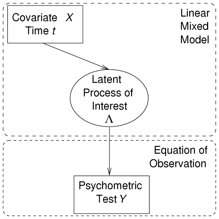
General Directed Graph of a Mixed Model for any Equation of Observation Between the Latent Process of Interest and the Psychometric Test.

For each statistical model, an equation of observation links the repeated measure of outcome Y_ij with the latent process level at the observation time t_ij, j representing the occasion (j=1, …, n_i):

• The standard LMM is obtained by assuming Y_ij=a + bΛ(t_ij) + ε_ij where ε_ij is an independent Gaussian measurement error at time t_ij and a and b are parameters to estimate that replace β₀ and variance of u_0i.

• The standard LMM applied on a pre-transformed outcome assumes similarly that h(Y_ij)=a + bΛ(t_ij) + ε_ij where h(.)is the pre-transformation (e.g. $h(\mathit{MMSE})=\sqrt{30-\mathit{MMSE}}$) and ε_ij, a and b are defined as above.

• In the latent process model proposed by Proust et al. (16) and called Beta LMM, the equation of observation is h(Y_ij,η)=a + bΛ(t_ij) + ε_ij where the transformation h(.,η) is a Beta cumulative distribution function depending on parameters η that are estimated along with the regression parameters and ε_ij, a and b are defined as above.

• In the threshold LMM, the equation of observation is defined at each level c of the outcome (c=0, …, C) by Y_ij=c⬄η_c≤Λ(t_ij)+ε_ij < η_c+1, where ε_ij is defined as above, thresholds η_c (c=1, …, C) are estimated along with the regression parameters and η₀ = −∞ and η_c+1=+∞ for identifiability (19).

Compared to the three former, the threshold LMM is computationally more intensive because of the increased number of parameters and the numerical integration required in the log-likelihood computation. However, as it models directly each possible level of the outcome, it is considered as the most adequate model among the candidates.

Goodness-of-fit of these four models was compared in the natural scale of the outcome using the Akaike information criterion (AIC) (27). To make possible the comparison of models assuming continuous (standard, pre-transformed and Beta LMM) and discrete data (threshold LMM), the posterior likelihood was computed as the probability of observing the discrete values from estimated standard, pre-transformed and Beta LMM rather than the density (details in Appendix).

RESULTS

Illustration on data from PAQUID cohort

Histograms of the four psychometric tests distributions are given in Figure 2 for GA and PDPD samples. With exception for the IST, they underline asymmetric and bounded distributions that could reflect curvilinearity problems and justify the use of more sophisticated mixed models.

Figure 2.

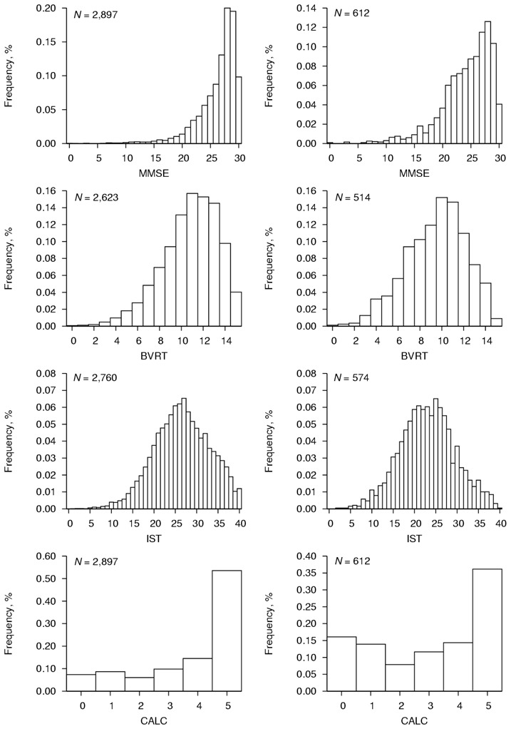
Distributions of Four Psychometric Tests in General Aging (on the left) and in Pre-Diagnostic Phase of Dementia (on the right) pooled from all available visits, PAQUID study, 1989–2004, France. MMSE, BVRT, IST and CALC respectively refer to Mini Mental State Examination, Benton Visual Retention Test, Isaacs Set Test and CALCulation subscore of MMSE. N indicates the Number of Subjects. The Median Number of Visits per Subject for each Test is 3 (Interquartile Range 2–5).

Cognitive decline was studied according to age in GA samples, and time before dementia diagnosis in PDPD samples, and adjusted for educational level (EL) as a binary covariate (no diploma vs. graduated from primary school). The frequency of subjects with no diploma varied from 29.9% to 32.3% in GA samples, and from 39.1% to 43.1% in PDPD samples. Figure 3 displays estimated transformations linking the psychometric test with the underlying Gaussian latent process in each model considered, and Table 1 presents the corresponding AIC.

Figure 3.

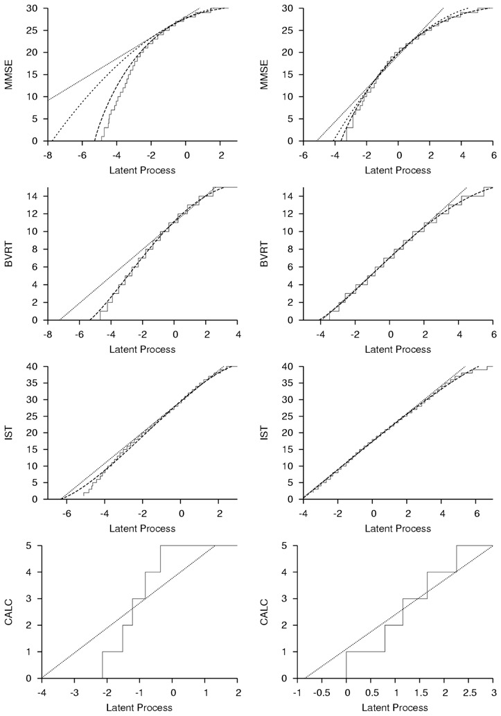
Estimated Transformations from Latent Process Linear Mixed Models (LMM) for the Four Psychometric Tests According to the Underlying Gaussian Latent Process in General Aging (on the left) and in Pre-Diagnostic Phase of Dementia (on the right), PAQUID study, 1989–2004, France. Solid Line Denotes the Threshold LMM, Dashed Line Denotes the Beta LMM, Dotted Line Denotes the Standard LMM and Dash-dotted Line Denotes the Pre-transformed LMM Used for MMSE only. MMSE, BVRT, IST and CALC Respectively Refer to Mini Mental State Examination, Benton Visual Retention Test, Isaacs Set Test and CALCulation subscore of MMSE. Number of Subjects and Median Number of Visits per Subject are Given in Figure 2.

Table 1.

Akaike Criterion Computed for Ordinal Data From the Mixed Models with Educational Level as Predictor in General Aging and Pre-Diagnostic Phase of Dementia Samples, PAQUID study, 1989–2004, France. Number of Subjects and Median Number of Visits per Subject are Given in Figure 2.

Sample	Model	MMSE	BVRT	IST	CALC
General Aging	Standard LMM	45418.8	38682.2	57139.0	25738.6
	Pre-transformed LMM	41944.4
	Beta LMM	41235.8	38148.2	57105.3
	Threshold LMM	41141.5	38141.8	56997.5	23191.6
Pre-Diagnostic Phase of Dementia	Standard LMM	10075.1	7333.9	11114.9	5825.8
	Pre-transformed LMM	9560.8
	Beta LMM	9499.0	7268.1	11108.9
	Threshold LMM	9483.5	7270.5	11127.4	5391.8

Abbreviations: BVRT, Benton Visual Retention Test; CALC, calculation subscore of MMSE; IST, Isaacs Set Test; LMM, Linear Mixed Model; MMSE, Mini-Mental State Examination.

For MMSE, in both samples, the standard LMM assumed a linear transformation very far from the nonlinear one estimated by the most flexible threshold LMM, and the difference in AIC (ΔAIC) between the models reached 4,227 points in GA and 592 points in PDPD. If the use of a pre-transformation shrank this gap, it remained quite important with a ΔAIC of 803 points in GA and 77 points in PDPD. In contrast, the estimated transformation from the Beta LMM was close to the transformation stemmed from the threshold LMM showing that it constituted a good alternative. This was confirmed by a largely reduced difference of AIC in GA (ΔAIC=94) and in PDPD (ΔAIC=16).

For BVRT, in GA sample, the linear transformation assumed in the standard LMM was relatively far from the transformation estimated in the threshold LMM (with ΔAIC=540). In PDPD sample, transformations from the threshold and standard LMM were relatively close in low levels of the tests. However, they differed in high levels and the ΔAIC of 63 points indicated again a better fit of the threshold LMM. In contrast, the transformations from the Beta LMM remained very close to the ones estimated in the threshold LMM in both samples, and the fit were very similar (AIC of Beta LMM was 2.4 points better in PDPD and 6.4 points worse in GA).

For IST, the linear transformation assumed in the standard LMM was close to the ones estimated in the Beta and threshold LMM in both GA and PDPD samples. In GA sample, a slight difference in the transformations could be observed in very small values of IST. Although this corresponded to few observations (see Figure 2), this lead to a better AIC for the threshold model than for the Beta (ΔAIC=108) and standard (ΔAIC=142) LMM. In PDPD sample in contrast, parsimonious Beta and standard LMM gave better AIC (respectively ΔAIC=19 and ΔAIC=13) with a slight preference for Beta LMM.

For CALC, large differences in the estimated transformations from the standard and threshold LMM were observed in GA. They were reduced but still present in PDPD. The ΔAIC reached 2,547 points in GA and 434 points in PDPD which indicated the markedly better fit of the model accounting for the discrete nature of the test. The Beta LMM was not applied with CALC. Indeed a model assuming continuous data is not appropriate for a test with 6 levels and may induce convergence problems (this comment applies to the standard LMM too).

These analyses showed that flexible models accounting for the test curvilinearity gave markedly better fits. Not surprisingly these differences resulted in parameter estimates of EL impact on cognitive baseline level and cognitive rate of change that were quite different (see Table 2). However, they also resulted in markedly different parameter p-values that even induced dissimilar conclusions regarding EL association with cognitive decline (interaction EL*t). For example in GA sample, the threshold LMM accounting for curvilinearity did not highlight any interaction between EL and cognitive decline for MMSE, BVRT and CALC while significant associations were found when using a standard LMM. These contradictions regarding EL effect did not necessarily emerge in the predicted trajectories of cognitive decline represented in figure 4: the trajectories remained relatively close in the threshold LMM and the standard LMM. Indeed, the curvilinearity means that the intensity of change represented by one point lost in the test varies as the test level changes. Consequently, although the distance in latent cognitive level between high and low EL remained the same across time and range of latent cognition (no interaction with time), the distance between high and low EL in the test scale varied with time and initial levels of the test. When assuming a constant intensity of change in the entire range of the test, that is using the standard LMM, this non constant gap between high and low EL was translated into a fake interaction with time.

Table 2.

Estimates (and P-values from the Wald Test) of Educational Level (EL) Effect on Baseline (EL) and Slope (EL × t) for Different Mixed Models in General Aging and Pre-Diagnostic Phase of Dementia Samples, PAQUID, 1989–2004, France. Number of Subjects and Median Number of Visits per Subject are Given in Figure 2.

Psychometric test	Estimated Model	General Aging				Pre-Diagnostic Phase of Dementia
		ELa		EL × ta,b		ELa		EL × ta,b
		Estimate	(P value)c	Estimate	(P value)c	Estimate	(P value)c	Estimate	(P value)c
MMSE	standard LMM	0.618	(<0.0001)	0.389	(<0.0001)	0.761	(<0.0001)	0.0184	(0.178)
	ptr LMM	0.909	(<0.0001)	0.238	(<0.0001)	0.92	(<0.0001)	−0.007	(0.675)
	Beta LMM	1.026	(<0.0001)	0.114	(0.034)	1.022	(<0.0001)	−0.0242	(0.180)
	Threshold LMM	1.000	(<0.0001)	0.092	(0.067)	1.011	(<0.0001)	−0.028	(0.134)
BVRT	standard LMM	1.067	(<0.0001)	0.151	(0.029)	0.816	(<0.0001)	−0.0186	(0.295)
	Beta LMM	1.033	(<0.0001)	0.03	(0.618)	0.863	(<0.0001)	−0.0285	(0.156)
	Threshold LMM	1.04	(<0.0001)	0.02	(0.621)	0.862	(<0.0001)	−0.0295	(0.146)
IST	standard LMM	1.031	(<0.0001)	−0.085	(0.0836)	0.433	(0.0001)	−0.036	(0.0199)
	Beta LMM	1.038	(<0.0001)	−0.131	(0.0050)	0.437	(0.0001)	−0.043	(0.0094)
	Threshold LMM	1.017	(<0.0001)	−0.148	(0.0008)	0.439	(<0.0001)	−0.042	(0.0079)
CALC	standard LMM	1.241	(<0.0001)	0.288	(<0.0001)	1.196	(<0.0001)	−0.005	(0.730)
	Threshold LMM	1.09	(<0.0001)	0.037	(0.453)	1.198	(<0.0001)	−0.045	(0.016)

Abbreviations: BVRT, Benton Visual Retention Test; CALC, calculation subscore of MMSE; EL, Educational Level; IST, Isaacs Set Test; LMM, Linear Mixed Model; MMSE, Mini-Mental State Examination; t, Time.

^ano diploma in reference

^btime t corresponds to age in decades from 65 in the general aging sample and years before diagnosis in pre-diagnostic phase of dementia sample.

^cP value from the Wald test

Figure 4.

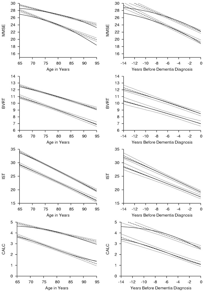
Predicted Trajectories of Cognitive Decline According to Educational Level for the Four Psychometric Tests in General Aging (on the left) and Pre-Diagnostic Phase of Dementia (on the right) using the Standard Linear Mixed Model (in Dashed Lines, and 95% Confidence Bands in Dotted Lines) and the Threshold Linear Mixed Model (in Solid Line). In each Graph, the Top Trajectories Correspond to Higher Educational Level and the Bottom Trajectories Correspond to Lower Educational Level, PAQUID study, 1989–2004, France. MMSE, BVRT, IST and CALC Respectively Refer to Mini Mental State Examination, Benton Visual Retention Test, Isaacs Set Test and CALCulation subscore of MMSE. Number of Subjects and Median Number of Visits per Subject are Given in Figure 2.

This kind of departure from the LMM assumptions is very difficult to highlight in diagnostic analyses. For example, except for MMSE and CALC in GA, the subject-specific residuals from the standard LMM displayed in Figure 5 with quantile-quantile plots did not show any severe departure from the Normality assumption. It was the same for other diagnostic tests. Only the analysis of a better suited model revealed the problem with curvilinearity.

Figure 5.

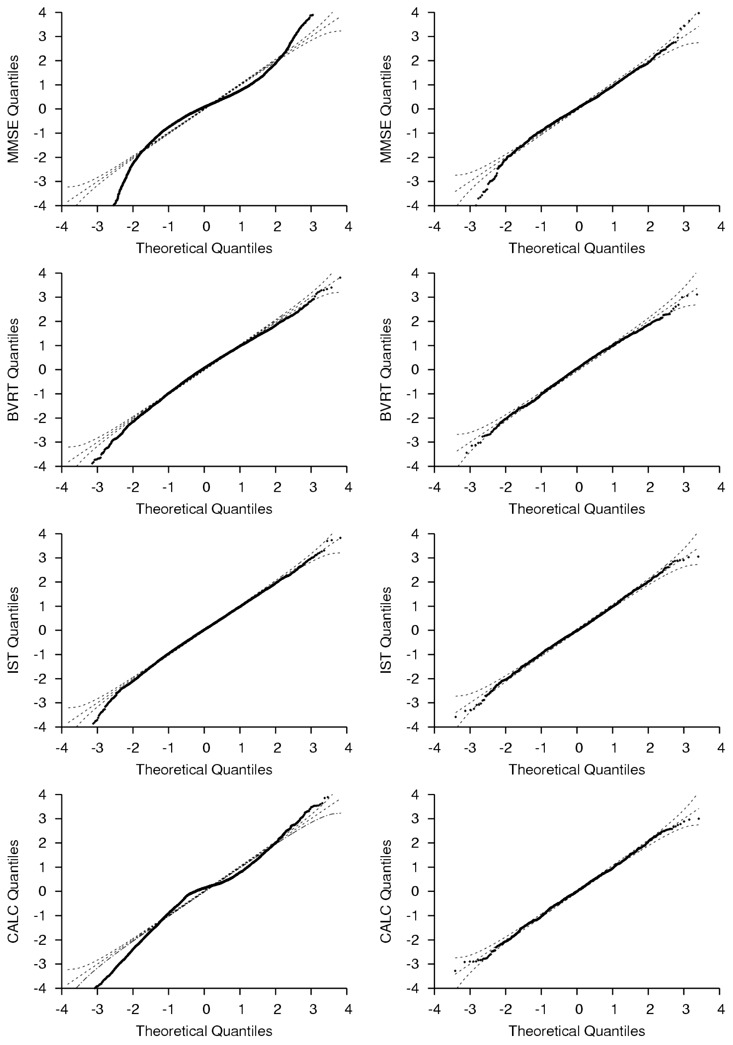
Quantile-Quantile Plots of Subject-Specific Standardized Residuals (with 95% Confidence Bands) for the Four Psychometric Tests in General Aging (on the left) and Pre-Diagnostic Phase of Dementia (on the right) using the Standard Linear Mixed Model, PAQUID study, 1989–2004, France. MMSE, BVRT, IST and CALC Respectively Refer to Mini Mental State Examination, Benton Visual Retention Test, Isaacs Set Test and CALCulation subscore of MMSE. Number of Subjects and Median Number of Visits per Subject are Given in Figure 2.

Simulation study

Motivated by these observations, a simulation study was performed to evaluate the impact of a misspecification of the LMM when testing regression parameters. We specifically investigated whether the tests for covariate effect on baseline level and slope were biased. Samples were simulated from the most flexible model that is the threshold LMM with parameter values fixed at point estimates of the illustration samples. Sixteen scenarios were investigated. The four psychometric test distributions were mimicked and called respectively mim-MMSE, mim-BVRT, mim-IST and mim-CALC. Two binary covariates were considered. X₁ corresponded to EL effect on the psychometric tests. As EL had a strong effect on baseline level and no effect on the slope, X₂ was also simulated with half the effect of EL on the intercept and four times the effect of EL on the slope to explore different types of association. Two kinds of samples were finally generated using parameters estimated on GA and PDPD samples. The time scale was age for GA (transformed to (age–65)/10) and years before diagnosis for PDPD. Simulation design is detailed in Appendix. For mim-MMSE, 4 mixed models were compared: the standard LMM, the pre-transformed LMM (where $h(\mathit{MMSE})=\sqrt{31}-\sqrt{31-\mathit{MMSE}}$ imitates the transformation $\sqrt{30-\mathit{MMSE}}$ but avoiding derivation problems in MMSE=30 and retaining the same direction as MMSE), the Beta LMM and the threshold LMM. For mim-BVRT and mim-IST only the standard, Beta and threshold LMM were considered as there were no usual pre-transformations for these tests. For mim-CALC, only the standard and threshold LMM were considered.

For each scenario, 500 samples of 500 subjects were simulated. Table 3 gives the estimated type I error (α̂ ) of the Wald test for the covariate effect on baseline (X) and interaction with time (X*t) for a nominal value of α=5%. The estimated type I error of the Wald test was obtained by simulating the samples with a 0 parameter value and calculating the percentage of times where this parameter was found significantly different from 0 using the Wald test. This corresponds to test a baseline effect in a model where there is only an interaction effect and inversely. In a well-specified model, α̂ is close to 5%.

Table 3.

Estimated Type I Error from the Wald Test (α̂ given in %) of Regression Parameter For Covariate X₁ or X₂ and Interaction With Time From 500 Replicated Samples of 500 Subjects in General Aging and Pre-Diagnostic Phase of Dementia.

Outcome distribution	Estimated Model	General Aging				Pre-Diagnostic Phase of Dementia Sample
		X1	X1× ta	X2	X2 × ta	X1	X1 × ta	X2	X2 × ta
mim-MMSE	Standard LMM	5.0	93.2b	33.6b	40.0b	4.8	97.8b	11.4b	54.0b
	Pre-transformed LMM	3.6	40.8b	7.2b	13.0b	4.6	42.6b	6.0	13.0b
	Beta LMM	4.4	4.6	4.0	4.2	4.4	6.2	4.6	6.0
mim-BVRT	Standard LMM	3.2	21.4b	4.4	8.6b	4.6	12.2b	5.4	8.6b
	Beta LMM	3.8	6.0	5.4	5.0	4.6	5.0	5.0	6.6
mim-IST	Standard LMM	4.6	8.0b	6.6	4.8	4.2	6.0	6.2	5.6
	Beta LMM	4.6	5.0	5.6	4.6	4.2	4.6	6.4	4.8
mim-CALC	Standard LMM	5.0	45.6b	6.4	5.2	4.2	56.4b	26.0b	5.6
	Threshold LMM	6.4	5.2	6.2	5.2	5.2	6.6	5.6	5.4

Abbreviations: LMM, Linear Mixed Model; mim-BVRT, distribution mimicking Benton Visual Retention Test; mim-CALC, distribution mimicking calculation subscore of MMSE; mim-IST, distribution mimicking Isaacs Set Test; mim-MMSE, distribution mimicking Mini-Mental State Examination; t, Time.

^atime t corresponds to age in decades from 65 in the general aging sample and years before diagnosis in pre-diagnostic phase of dementia sample.

^bestimated type I errors (α̂ ) outside the expected 95% interval 3.09, 6.91 around the nominal value of 5%.

For mim-MMSE, α̂ reached 93.2% in GA or 97.8% in PDPD for interaction between X₁ and time when using standard LMM. This indicates that the standard LMM concludes there is an interaction 93.2% (or 97.8%) of the times when there is no interaction. When using the pre-transformation, α̂ was reduced but still far from the nominal value with more than 40.8% for X₁*t, and 13.0% for X₂*t. In contrast, using the Beta LMM, α̂ were close to 5%. In any mixed model, α̂ for X₁ effect on baseline level were close to 5% Indeed, as the interaction X₁*t was nearly 0, it could not blur the association with baseline effect.

For mim-BVRT, the standard LMM worked better than for mim-MMSE. However, α̂ reached 21.4% for some interactions between the covariate and the time. In contrast, the Beta LMM again gave good results.

For mim-CALC, α̂ were high in the standard LMM for interaction between X₁ and time (45.6% in GA and 56.4% in PDPD) and for X₂ effect on baseline in PDPD (26.0%) while the threshold LMM gave good results (it was the correct model).

Finally, for mim-IST that highlighted a relatively linear transformation in figure 3, α̂ were close to 5% in the standard and Beta LMM

DISCUSSION

This work aimed at demonstrating that the standard LMM used on psychometric tests could lead to spurious associations of risk factors with cognitive change over time. Our conclusions were based on four psychometric tests that are largely used in epidemiological studies and exhibit different types of distribution, as well as two distinct populations. With exception for the IST, the illustration highlighted that the standard LMM provided a markedly worse fit of the data than the threshold LMM specifically adapted to discrete and bounded data or the Beta LMM that accounted for curvilinearity while considering the data as continuous (16). Indeed, the estimated transformations derived from these models showed a clear nonlinear relationship between each test and the underlying biological process of interest while the standard LMM assumed a linear transformation. This had been previously stated (8). The simulation study provided further arguments to demonstrate that for three of the psychometric tests, the associations with covariates in the standard LMM were distorted. In particular, when the risk factor had an effect on the initial cognitive level, the test for interaction with time was biased: it tended to conclude too many times to a spurious association between the risk factor and the rate of cognitive decline while there was only an association with the initial level. This comes from the curvilinearity of the tests. The test varying sensitivity to change induces a varying distance between two groups even when there is no interaction with time. By neglecting the test curvilinearity, the standard LMM interprets this varying distance as an interaction with time, so that confusion appears between the risk factor impact on the initial level and its impact on cognitive change with time. Such confusion can be of great importance. For example, if educational level, a proxy of reserve capacity of the brain, was found related to decline of a given test, the authors concluded that reserve capacities were particularly linked to the underlying cognitive function without considering the misuse of the model. Curvilinearity constitutes an intrinsic property of the test that should be accounted for in any regression model whatever the studied population, the covariates or the time scale. Especially, it cannot be corrected by changing the time scale or adding nonlinear covariate effects. For instance, the estimated nonlinear transformations in both Paquid datasets were almost identical when rescaling the latent process, and were practically not changed when considering quadratic trajectories or when removing the covariate (results not shown).

Recommendations should be addressed based on these findings. In any analysis evaluating risk factors on a psychometric test change over time, the standard LMM should not be used without a precise inspection of the psychometric test properties. In particular, a more adequate mixed model that accounts for curvilinearity and ceiling/floor effects should be estimated to evaluate the violation of the LMM assumptions and the reliability of the associations highlighted. For many psychometric tests like MMSE and BVRT, the standard LMM is most likely not reliable, and mixed model that accounts for curvilinearity should be systematically preferred. The threshold mixed model is the most reliable model as it models directly each level of the outcome but it is computationally intensive. Therefore, for psychometric tests including a relatively large number of levels, a model assuming a curvilinear continuous outcome can be used instead. For example, the Beta LMM (16) provided similar fits as the threshold LMM and more importantly gave unbiased inference in our simulations while avoiding the computational problems. In contrast, for psychometric tests with a small number of levels, the threshold LMM should be preferred. The 1 cmm user-friendly R function is available within the 1 cmm R package (http://cran.r-project.org/web/packages/lcmm/) for estimating latent process LMM including threshold and Beta LMM, and SAS macros are available on http://biostat.isped.u-bordeaux2.fr.

The main concern regarding alternative mixed models is that, in contrast with the LMM, they do not provide an interpretation of risk factor impact in terms of a number of points lost on the test scale per time unit. This is actually a direct consequence of curvilinearity: one point lost in a test scale does not have the same meaning on the whole test range, it depends on the initial level. So if significance degree and direction of associations can be still interpreted like in the LMM, the intensity of association should be rather appreciated graphically as in figure 4 or be quantified in the psychometric test scale in terms of the number of years a subject with a certain covariate value would need to reach the same cognitive level as a person with the covariate reference value (28). For example, in the illustration, a subject with high EL would reach the same MMSE as a subject with low EL 14.7 years later at 65 years old, and respectively 13.9 and 12.9 years later at 70 and 75 years old. In contrast, when using the standard LMM, the estimated effect corresponds to respectively 8.1, 10.9 and 13.1 at 65, 70 and 75 years old.

In conclusion, to distinguish impact of a covariate on the initial level from its impact on the change over time of quantitative scales, such as psychometric tests but also quality of life or activities of daily living scales, mixed models that account for their metrological properties should be preferred to the linear mixed model.

Abbreviates

LMM

Linear Mixed Model

MMSE

Mini Mental State Examination

IRT

Item Response Theory

CALC

calculation subscore of the MMSE

BVRT

Benton Visual Retention Test

IST

Isaacs Set Test

PDPD

pre-diagnostic phase of dementia

GA

general aging

EL

educational level

AIC

Akaike information criterion

ΔAIC

difference in AIC

APPENDIX

1. Computation of Akaike’s information criterion for discrete data

Using the latent process model formulation, the probability of observing the value k of an ordinal outcome Y with values in {0, …, C} is:

$$P(Y_{ij}=k)=P({\kappa }_k\le \mathrm{\Lambda }(t_{ij})+{\epsilon }_{ij}<{\kappa }_{k+1})\text{with}{\kappa }_0=-\infty \text{and}{\kappa }_{C+1}=+\infty$$ (2)

for subject i, i=1, …, N and occasion j, j=1, … n_i.

In a threshold model that considers an ordinal outcome, the thresholds κ_k for k=1, …, C are directly estimated. To compute the likelihood for the ordinal outcome using the other estimated mixed model that consider Y as continuous, equation (2) was also used with thresholds κ_k (k=1, …, C) defined as κ_k=k+0.5 in the standard LMM, ${\kappa }_k=\frac{h(k)+h(k+1)}{2}$ in the pre-transformed LMM and ${\kappa }_k=\frac{h(k,\widehat{\eta })+h(k+1,\widehat{\eta })}{2}$ in the Beta LMM (with η̂ the maximum likelihood estimate of η).

2. design of the simulation study

Samples were simulated to mimic the PAQUID cohort. Entry in the cohort was simulated according to a uniform distribution between [65;80] years old for GA and [−14; −7] years before diagnosis for PDPD while dropout was simulated according to a uniform distribution between [80;95] years old for GA and fixed at time 0 for PDPD. In this window, each subject had a measure every 3 years. The binary covariate (X₁ or X₂) was simulated according to a Bernoulli with a 0.5 probability.

References

- 1.Butler SM, Louis TA. Random effects models with non-parametric priors. Stat Med. 1992;11(14–15):1981–2000. doi: 10.1002/sim.4780111416. [DOI] [PubMed] [Google Scholar]
- 2.Verbeke G, Lesaffre E. The effect of misspecifying the random-effects distribution in linear mixed models for longitudinal data. Computational Statistics & Data Analysis. 1997;23(4):541–556. [Google Scholar]
- 3.Zhang D, Davidian M. Linear mixed models with flexible distributions of random effects for longitudinal data. Biometrics. 2001;57(3):795–802. doi: 10.1111/j.0006-341x.2001.00795.x. [DOI] [PubMed] [Google Scholar]
- 4.Jacqmin-Gadda H, Sibillot S, Proust C, et al. Robustness of the linear mixed model to misspecified error distribution. Computational Statistics & Data Analysis. 2007;51(10):5142–5154. [Google Scholar]
- 5.Liang K-Y, Zeger SL. Longitudinal data analysis using generalized linear models. Biometrika. 1986;73(1):13–22. [Google Scholar]
- 6.Taylor JMG, Cumberland WG, Sy JP. A stochastic model for analysis of longitudinal AIDS data. Alexandria, VA: ETATS-UNIS: American Statistical Association; 1994. [Google Scholar]
- 7.Morris MC, Evans DA, Hebert LE, et al. Methodological issues in the study of cognitive decline. Am J Epidemiol. 1999;149(9):789–793. doi: 10.1093/oxfordjournals.aje.a009893. [DOI] [PubMed] [Google Scholar]
- 8.Proust-Lima C, Amieva H, Dartigues JF, et al. Sensitivity of four psychometric tests to measure cognitive changes in brain aging-population-based studies. Am J Epidemiol. 2007;165(3):344–350. doi: 10.1093/aje/kwk017. [DOI] [PMC free article] [PubMed] [Google Scholar]
- 9.Folstein MF, Folstein SE, McHugh PR. “Mini-mental state”. A practical method for grading the cognitive state of patients for the clinician. J Psychiatr Res. 1975;12(3):189–198. doi: 10.1016/0022-3956(75)90026-6. [DOI] [PubMed] [Google Scholar]
- 10.Feng L, Li J, Yap KB, et al. Vitamin B-12, apolipoprotein E genotype, and cognitive performance in community-living older adults: evidence of a gene-micronutrient interaction. Am J Clin Nutr. 2009;89(4):1263–1268. doi: 10.3945/ajcn.2008.26969. [DOI] [PubMed] [Google Scholar]
- 11.Rolland Y, Abellan van Kan G, Nourhashemi F, et al. An abnormal “one-leg balance” test predicts cognitive decline during Alzheimer’s disease. J Alzheimers Dis. 2009;16(3):525–531. doi: 10.3233/JAD-2009-0987. [DOI] [PubMed] [Google Scholar]
- 12.Stott DJ, Falconer A, Kerr GD, et al. Does low to moderate alcohol intake protect against cognitive decline in older people? J Am Geriatr Soc. 2008;56(12):2217–2224. doi: 10.1111/j.1532-5415.2008.02007.x. [DOI] [PubMed] [Google Scholar]
- 13.Sanders AE, Wang C, Katz M, et al. Association of a functional polymorphism in the cholesteryl ester transfer protein (CETP) gene with memory decline and incidence of dementia. JAMA. 2010;303(2):150–158. doi: 10.1001/jama.2009.1988. [DOI] [PMC free article] [PubMed] [Google Scholar]
- 14.Jacqmin-Gadda H, Fabrigoule C, Commenges D, et al. A 5-year longitudinal study of the Mini-Mental State Examination in normal aging. Am J Epidemiol. 1997;145(6):498–506. doi: 10.1093/oxfordjournals.aje.a009137. [DOI] [PubMed] [Google Scholar]
- 15.Ganiayre J, Commenges D, Letenneur L. A latent process model for dementia and psychometric tests. Lifetime Data Anal. 2008;14(2):115–133. doi: 10.1007/s10985-007-9057-x. [DOI] [PubMed] [Google Scholar]
- 16.Proust C, Jacqmin-Gadda H, Taylor JM, et al. A nonlinear model with latent process for cognitive evolution using multivariate longitudinal data. Biometrics. 2006;62(4):1014–1024. doi: 10.1111/j.1541-0420.2006.00573.x. [DOI] [PMC free article] [PubMed] [Google Scholar]
- 17.Jacqmin-Gadda H, Proust-Lima C, Amieva H. Semi-parametric model for ordinal longitudinal data. Stat Med. 2010;29(26):2723–2731. doi: 10.1002/sim.4035. [DOI] [PubMed] [Google Scholar]
- 18.Crane PK, Narasimhalu K, Gibbons LE, et al. Item response theory facilitated cocalibrating cognitive tests and reduced bias in estimated rates of decline. J Clin Epidemiol. 2008;61(10):1018–1027. e9. doi: 10.1016/j.jclinepi.2007.11.011. [DOI] [PMC free article] [PubMed] [Google Scholar]
- 19.Liu LC, Hedeker D. A mixed-effects regression model for longitudinal multivariate ordinal data. Biometrics. 2006;62(1):261–268. doi: 10.1111/j.1541-0420.2005.00408.x. [DOI] [PubMed] [Google Scholar]
- 20.Mungas D, Harvey D, Reed BR, et al. Longitudinal volumetric MRI change and rate of cognitive decline. Neurology. 2005;65(4):565–571. doi: 10.1212/01.wnl.0000172913.88973.0d. [DOI] [PMC free article] [PubMed] [Google Scholar]
- 21.Rijmen F, Tuerlinckx F, De Boeck P, et al. A nonlinear mixed model framework for item response theory. Psychol Methods. 2003;8(2):185–205. doi: 10.1037/1082-989x.8.2.185. [DOI] [PubMed] [Google Scholar]
- 22.Hedeker D, Gibbons RD. A random-effects ordinal regression model for multilevel analysis. Biometrics. 1994;50(4):933–944. [PubMed] [Google Scholar]
- 23.Letenneur L, Commenges D, Dartigues JF, et al. Incidence of dementia and Alzheimer’s disease in elderly community residents of south-western France. Int J Epidemiol. 1994;23(6):1256–1261. doi: 10.1093/ije/23.6.1256. [DOI] [PubMed] [Google Scholar]
- 24.Benton A. Manuel pour l’application du Test de Rétention Visuelle. Applications cliniques et expérimentales. Paris: Centre de Psychologie appliquée; 1965. 2ème édition française ed. [Google Scholar]
- 25.Isaacs B, Kennie AT. The Set test as an aid to the detection of dementia in old people. Br J Psychiatry. 1973;123(575):467–470. doi: 10.1192/bjp.123.4.467. [DOI] [PubMed] [Google Scholar]
- 26.Laird NM, Ware JH. Random-effects models for longitudinal data. Biometrics. 1982;38(4):963–974. [PubMed] [Google Scholar]
- 27.Akaike H. A new look at the statistical model identification. IEEE Transactions on Automatic Control. 1974;19 (6):716–723. [Google Scholar]
- 28.Proust-Lima C, Amieva H, Letenneur L, et al. Gender and education impact on brain aging: a general cognitive factor approach. Psychol Aging. 2008;23(3):608–620. doi: 10.1037/a0012838. [DOI] [PubMed] [Google Scholar]