The Use of Laser-Induced Breakdown Spectroscopy for Distinguishing Between Bacterial Pathogen Species and Strains

Abstract

Laser-induced breakdown spectroscopy (LIBS) was used in a blind study to successfully differentiate bacterial pathogens, both species and strain. The pathogens used for the study were chosen and prepared by one set of researchers. The LIBS data were collected and analyzed by another set of researchers. The latter researchers had no knowledge of the sample identities other than that (1) the first five of fifteen samples were unique (not replicates) and (2) the remaining ten samples consisted of two replicates of each of the first five samples. Using only chemometric analysis of the LIBS data, the ten replicate bacterial samples were successfully matched to each of the first five samples. The results of this blind study show it is possible to differentiate the bacterial pathogens Escherichia coli, three clonal methicillin-resistant Staphylococcus aureus (MRSA) strains, and one unrelated MRSA strain using LIBS. This is an important finding because it demonstrates that LIBS can be used to determine bacterial pathogen species within a defined sample set and can be used to differentiate between clonal relationships among strains of a single multiple-antibiotic-resistant bacterial species. Such a capability is important for the development of LIBS instruments for use in medical, water, and food safety applications.

INTRODUCTION

Laser-induced breakdown spectroscopy (LIBS) is a spectroscopic analysis technique in which a laser pulse vaporizes nanogram to microgram quantities of material and thermally excites the vaporized material in a short-lived plasma (~8000 K). Light emitted from atoms, ions, and simple molecules in the plasma is collected and analyzed. Traditionally, LIBS is an elemental analysis technique used to determine the composition of the target material via unique elemental fingerprint spectra. More recently, chemometric¹ or other analysis techniques have been applied to LIBS spectra for both classification and identification of various materials. In these cases, the entire LIBS spectrum is used for identification of materials as opposed to particular elemental lines.

The LIBS technique has been used in many applications, including compositional analysis of rocks and soils, detection of explosives, sorting of metals, and trace element detection in aerosols, liquids, and solids.^2–4 Most recently, LIBS has also been investigated as a tool for detecting and identifying biological material. Morel et al. demonstrated that LIBS could detect and sort species using six bacteria and two pollens in pellet form.⁵ Guyron et al. studied the differences in LIBS bacterial spectra for both ns-LIBS and fs-LIBS.⁶ Rehse et al. and Diedrich et al. have shown that both pathogenic and non-pathogenic Escherichia coli (E. coli) cultured strains grown in both nutrient-rich and nutrient-free media can be differentiated using discriminative functional analysis (DFA) on LIBS spectra.^7–9 Both Gottfried et al. and Snyder et al. have shown that LIBS can be used to differentiate biological warfare simulants in a defined sample set. Gottfried et al. demonstrated discrimination using both linear correlation and partial least squares regression discriminative analysis (PLS-DA) on LIBS spectral data preprocessed with respect to selected elemental lines.¹⁰ Snyder et al. demonstrated discrimination using multiple linear regression (MLR) and neural network analysis on LIBS data that was also preprocessed.¹¹ Work has also been done using principal component analysis (PCA) and neural networks on LIBS data to detect hazardous biological materials using both laboratory size and miniaturized LIBS experimental components.¹²

To our knowledge, the work presented here is the first use of LIBS to discriminate pure, viable pathogen samples based only on raw (unprocessed) LIBS spectra. It is also the first blind study demonstration showing that LIBS can be used to match unknown viable, pure pathogen species and strains to a defined sample set. This is an important result because LIBS has many advantages as a biosensing method for the identification of pathogenic microorganisms. These advantages include simplicity of use (focus the laser pulse on the material and collect the light), rapid in situ analysis (results in less than a minute), little or no sample preparation, and the feasibility of automated analysis. The ability to differentiate both species and strain using only raw spectra implies that LIBS shows promise for the development of instrumentation that could be used to support rapid medical diagnosis in both laboratory and field situations by personnel without any specific LIBS expertise.

For the blind study presented here, E. coli and four strains of Staphylococcus aureus (S. aureus) were chosen. Multiple-antimicrobial-resistant methicillin-resistant S. aureus (MRSA) causes serious infections in hospital patients and within the general populace, and MRSA demonstrating reduced susceptibility to the important antistaphylocccal drug vancomycin have been reported.¹³ Normally, numerous time-consuming culture-media-based and molecular biology techniques are required to differentiate common bacterial pathogens, resolve their clonal relationship among single specie strain collections, and determine antimicrobial resistance profiles.^14–16 Determining antimicrobial resistance phenotype is imperative when determining which antimicrobial regimen will best suit a diseased individual. In the present study, we demonstrate that LIBS can be used to differentiate the most common hospital-borne bacterial pathogens E. coli from S. aureus strains and to determine clonal relationships among well-characterized related and unrelated MRSA strains.

EXPERIMENTAL

The MRSA strains LP9, MM61, MM66, and MM66-4 utilized in this study have been previously described,¹⁴ and E. coli strain DH5α is commonly utilized for nucleic acid cloning procedures. Restriction fragment length polymorphism (RFLP) produced from pulsed field gel electrophoresis of infrequently cut SmaI-restricted chromosomal DNA, a gold standard for determining S. aureus strain evolutionary relatedness,¹⁷ demonstrated that strain LP9 was unrelated to strains MM61, MM66, and MM66-4.¹⁴ MM61 is 96% identical by SmaI-RFLP with low-level hetero-vancomycin intermediate S. aureus (hVISA) strain MM66, yet MM61 has an additional SmaI band of 80 kb and is vancomycin-susceptible.¹⁴ MM66-4 is a MM66 high-level vancomycin-intermediate S. aureus (VISA) mutant that was produced by plating MM66 onto nutrient plates containing 3 mg/L vancomycin and randomly picking surviving colonies.¹⁴

All bacterial cell samples were prepared by researchers at New Mexico State University (NMSU) by initially growing the cells in Luria–Bertani liquid media (Becton, Dickinson and Company, Sparks, MD) (37 °C, 200 rpm, flask to volume ratio: 10:1), harvested by centrifugation (8000 × g, 4 °C, 10 min), washed in cold phosphate buffered saline (pH 7.4), and then reharvested. The resulting cell pellets were frozen overnight at −80 °C in sterile lyophilization flasks, which were subsequently attached to a pre-cooled vacuum (−40 °C, 0.133 mBar) freeze-dry system (Labconco, Kansas City, MO) and lyophilized for 12 h. Lyophilized samples were then stored in a desiccator at 25 °C for 2 days and 0.5 mg samples were then placed in disposable plastic cuvettes (trUView, Bio-Rad laboratories, Inc. CA) for LIBS analysis.

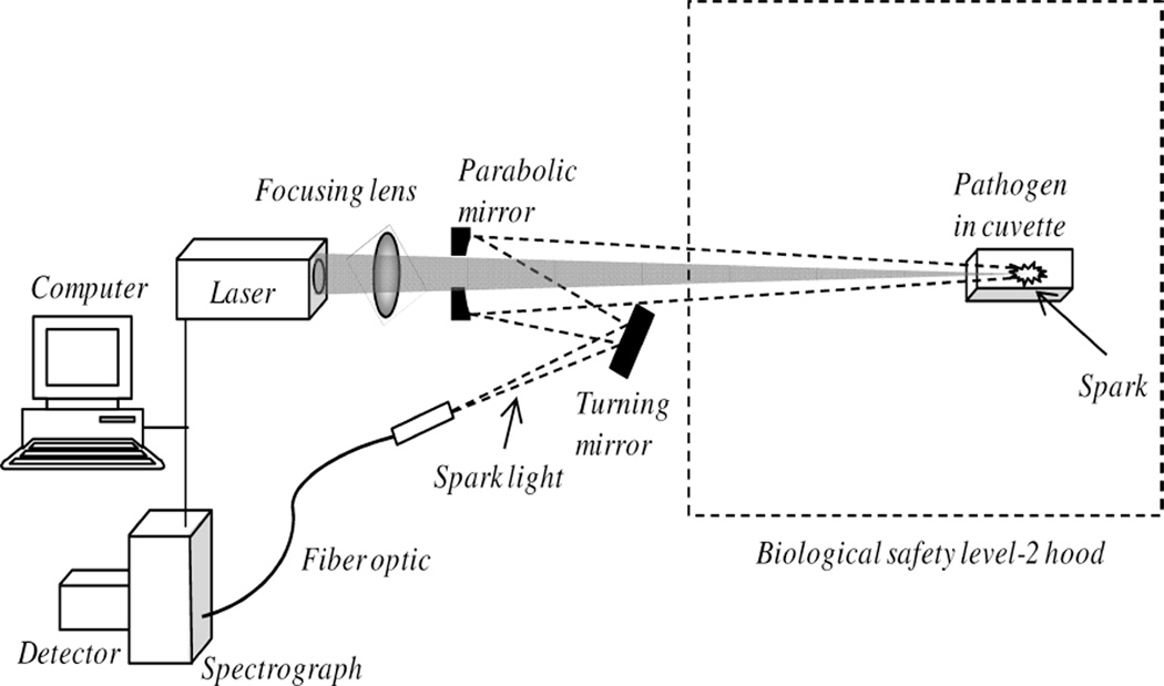
Researchers from Applied Research Associates, Inc. (ARA) were not told anything about the samples other than that each was a pathogen, the first five samples were unique, and that each of the remaining ten samples were replicates, two each, of the first five. All samples were labeled alphabetically (A–O) with samples A–E identified as the unique samples and samples F–O identified as the replicates. LIBS spectra were collected from the lyophilized bacterial samples using the experimental setup illustrated in Fig. 1.

Fig. 1.

Diagram of the experimental setup used to collect LIBS spectra of pathogens. The cuvette and pathogen sample were located inside a biological safety level-2 hood. LIBS emission was collected along the path of the laser light to remove parallax.

Each lyophilized pathogen sample was placed in a cuvette and pulses from a Q-switched Nd:YAG laser (1064 nm, 60 mJ/pulse, 10 Hz) were focused onto the sample by orienting the open cuvette end towards the laser and sparking the pathogen inside the cuvette. Data were collected with samples located in a biological safety level-2 hood. Plasma light was collected using an off-axis parabolic mirror and fiber optic and then routed to an echelle spectrometer (Catalina SE200 with Andor DH734-18F-03, I-Star intensified charge-coupled device (ICCD) camera). A hole in the parabolic mirror permitted the optical path of the laser pulses and light collection to be collinear, eliminating parallax. It should be noted that the lens-to-sample distance changed during interrogation because of the pressure waves created during sample ablation, which caused the lyophilized samples (powders) to move about within the cuvette. Each recorded spectrum represented the accumulation of ten spectra (camera acquisition parameters: 1 µs delay, 20 µs window) over an exposure period of 1 s. A total of 1050 individual spectra (70 spectra datasets for each sample) were collected for this study.

ANALYSIS

The analysis goal for this blind study was to determine whether LIBS plus chemometric analysis could be used to successfully match each of the samples F–O to one of samples A–E. Because the sample identities were unknown and to mimic an analysis situation in which data are collected and not controlled for quality, all collected spectra were used in the analysis with no screening for spectral quality and no data preprocessing. For each sample A–E, the 70 spectra collected were randomly separated into two sets: 50 spectra to be used in chemometric model building (classification set) and 20 to be used to test the performance of the various models (verification set). For the modeling, the entire wavelength range of the spectral data was used with each intensity measurement at each spectral wavelength treated as a variable value. Because the entire spectral range of 205.42 to 1000 nm was used (this range intentionally extends beyond the range of useful sample data, 205.42–850 nm), the modeling was done over 39 730 variables for each sample (205.42–1000 nm range, 0.02 nm resolution).

Various chemometric modeling methods such as PCA and projection to latent structures (PLS) regressions were applied to sample data sets A through E using commercially purchased analysis software (The Unscrambler, Camo Software Inc.). Each model was built using the classification spectra sets and tested on the verification spectra sets. Model performance was evaluated based on the percentage of verification set spectra that were matched correctly to the associated sample. After investigating multiple modeling methodologies, it was found that the best results were obtained using PLS2 for discrimination between two samples.

Projection to latent structures is a technique that generalizes and combines features from both PCA and multivariate regression. It is especially useful when trying to predict a set of dependent variables from a very large set of independent variables. In PLS analysis it is assumed that all of the measured variance is useful variance to be explained. The latent variables are estimated as exact linear combinations of the observed measures to create an exact definition of component scores. Through an iterative estimation technique, a general model is developed that encompasses canonical correlation, redundancy analysis, multiple regression, multivariate analysis of variance, and principal components. The iterative algorithm consists of a series of ordinary squares analyses. No distributional form is assumed for the measured variables. PLS2 is a PLS method in which several variables are modeled simultaneously to take advantage of possible correlations between the variables. Once a model has been generated for the sample classes, it can be used on test samples to produce a predictor value (in this case between 0 and 1) to be used to match the tested sample to one of the sample classes.

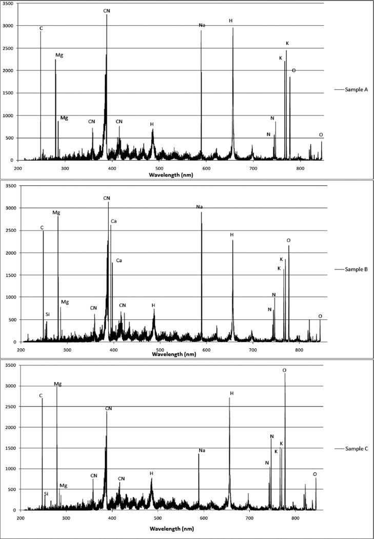
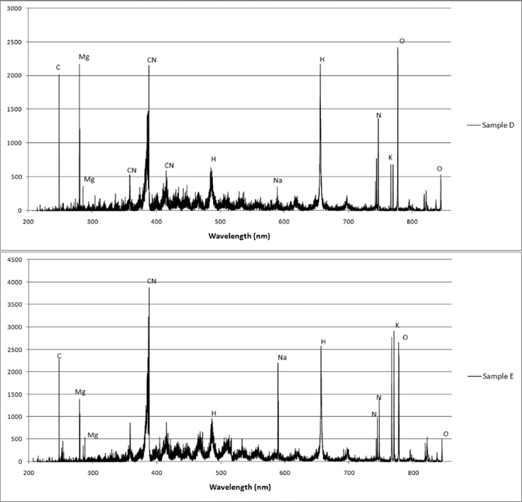
For this analysis, the dependent variable was the sample and the independent variables associated with the sample were the intensity measurements at each wavelength. Examples of LIBS classification set spectra obtained for samples A through E and used as input to create the PLS2 regression models are shown in Fig. 2. From these spectra, elemental compositional differences can be clearly seen. In all samples, spectral lines are present indicating the presence of C, Mg, Si, CN, H, K, O, Na, and N. Ca is observed only in sample B. The relative intensities of K and O vary for all samples and the most striking relative intensity difference is observed in sample D. These differences in elemental lines and their associated intensities contribute to the creation of a distinctive set of 39 730 variables for each sample.

Fig. 2.

Examples of LIBS classification spectra used for building models. The units of the ordinate axes are detector counts. True identities of the spectra are: sample A, S. aureus LP9; sample B, E. coli DH5α; sample C, S. aureus MM61; sample D, S. aureus MM66; and sample E, S. aureus MM66-4.

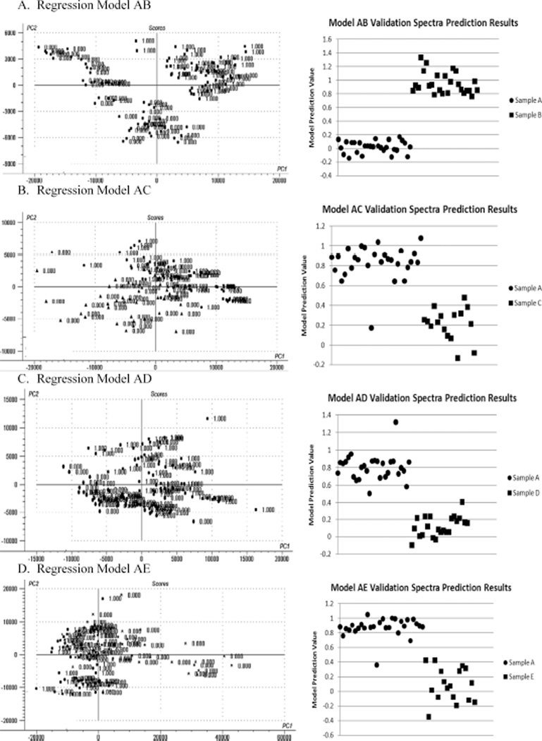
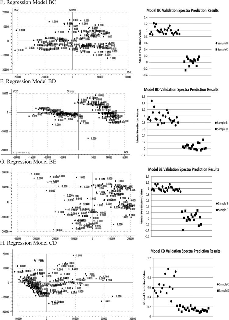
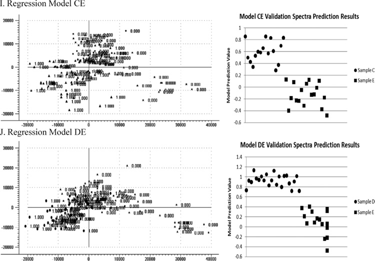
The goal of the analysis was to match each of the unknown samples to one of samples A–E. Because PLS2 regression analysis comparing one sample to another was found to have the best discrimination results, to cover every possible comparative combination of samples A through E, the following models were built: A vs. B (model AB), A vs. C (model AC), A vs. D (model AD), A vs. E (model AE), B vs. C (model BC), B vs. D (model BD), B vs. E (model BE), C vs. D (model CD), C vs. E (model CE), and D vs. E (model DE). Each model was built using the raw unprocessed spectra in the classification spectra sets and then tested on the verification spectra sets to verify discriminative performance. The score plot for the first two principal components (PC2 vs. PC1) for each model along with a plot of the results obtained when the model was tested on the verification sets is presented in Fig. 3. From examining the prediction value plots obtained for the verification data sets, it is clear that a discriminative prediction value can be chosen to separate the samples such that any sample with a larger prediction value could be associated with the first sample in the model and any sample with a lower prediction value could be associated with the second sample in the model.

Fig. 3.

Score plots for the first two principal components (PC2 vs. PC1) for each PLS2 regression model along with a plot of the prediction values obtained when the model was tested on the verification spectral sets. From the prediction value plots, it is clear that a prediction value can be chosen for each model to separate the two samples being compared.

The next step in the analysis was to understand how to apply the two sample comparative models to correctly match each of samples F–O with one of samples A–E. To do this, the following procedure was used: (1) each model was tested on the verification spectral set for each of the samples A–E; (2) the prediction values obtained for each spectra were averaged to produce a single prediction value for the verification set; (3) the average prediction value was compared to a selected discriminative prediction value (0.35 chosen) and the classification for each sample in each model was determined; (4) a table was made of the average prediction values and the sample classifications of each sample for each model (see Table I); (5) the table was studied to assess how each sample classified in each model; and (6) once the sample classification performance as a function of model was understood, a sample-matching algorithm using a subset of the comparative models was created to use in matching sample F through O to samples A through E.

TABLE I.

Average prediction values obtained for the verification spectra set of each sample A through E and the sample classification in each model.^a

Sample	Model	Average prediction value	Sample classification	Sample	Model	Average prediction value	Sample classification
A	AB	0.9743	A	B	AB	0.0697	B
	AC	0.8318	A		AC	0.2706	C
	AD	0.8046	A		AD	1.0978	A
	AE	0.8801	A		AE	0.7617	A
	BC	0.2535	C		BC	0.9806	B
	BD	0.2102	D		BD	0.9509	B
	BE	0.2879	E		BE	0.9759	B
	CD	0.4591	C		CD	0.7415	C
	CE	0.7884	C		CE	1.1540	C
	DE	0.6178	D		DE	0.1658	E
C	AB	0.9113	A	D	AB	0.9127	A
	AC	0.2130	C		AC	0.5575	A
	AD	0.5859	A		AD	0.1216	D
	AE	0.3549	A		AE	0.4902	A
	BC	0.0465	C		BC	0.0978	C
	BD	0.1997	D		BD	0.0579	D
	BE	0.1533	E		BE	0.3337	E
	CD	0.6275	C		CD	0.1519	D
	CE	0.5889	C		CE	0.5349	C
	DE	0.1742	E		DE	0.9287	D
E	AB	1.0023	A
	AC	0.6087	A
	AD	−0.0534	D
	AE	0.0887	E
	BC	0.0912	C
	BD	−0.0481	D
	BE	0.0425	E
	CD	0.4672	C
	CE	−0.1006	E
	DE	0.0945	E

^aThe key models used to match the unknown sample to one of the samples A through E are indicated in bold.

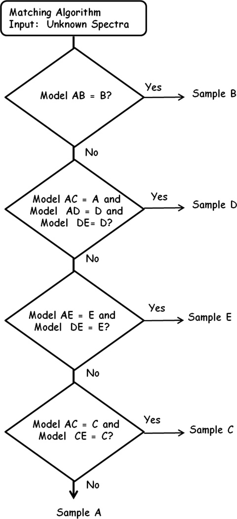
For the matching algorithm, it was found that model AB reliably identified sample B as “B”. So, the first step in the algorithm was to apply model AB. If the unknown sample was classified as “B” in the AB model, it was determined to be matched to sample B and no further testing was done. Sample D classified as sample “A” in the AC model, and as sample “D” in the AD and DE models. Therefore, the next step in the test flow was to apply models AC, AD, and AE. If the unknown classified as “A” in model AC, and as “D” in models AD and DE, then the sample was determined matched to sample D and no further testing was done. Sample E was classified as “E” in models AE and DE. Therefore, the third step in the testing flow was to apply models AE and DE. If the unknown sample classified as “E” in both of these models, then the sample was determined to be matched to sample E and no further testing was done. Sample C classified as “C” in models AC and CE. Therefore, the fourth step in the testing flow was to apply models AC and CE. If the unknown sample classified as “C” in both of these models, the sample was determined to be matched to sample C and no further testing was done. If the unknown sample was not matched in any of the above tests, it was determined to be matched to sample A. It should be noted that the order of applying the matching tests was critical to the success of the matching algorithm. A flowchart of the matching algorithm is presented in Fig. 4 and the elements or molecules with the highest contributions to regression coefficients of the models used in the algorithm may be found in Table II.

Fig. 4.

Flow chart of matching algorithm developed to match samples F through O to samples A through E.

TABLE II.

Elements with the highest contributions to the regression coefficients of the models used in the discrimination algorithm.

Model	Elements or molecules with highest contribution to regression coefficients (in order of highest to lowest influence left to right)
AB	Ca	O	C	Na	H
AC	Mg	C	O	Na	N
AD	Mg	C	O	CN	Na
DE	Mg	CN	H	C	Na
AE	O	N	C	Mg	CN
CE	Mg	C	O	CN	H

RESULTS

To match samples F through O to samples A through E, all 70 spectra collected for each sample were input into each model used in the matching algorithm and the results were then averaged. The discrimination prediction value used in the matching algorithm development was then applied to obtain the classification of each sample for each model (see Table III). The matching algorithm was then applied and the results were transmitted to the NMSU researchers for review. Using the matching methodology herein described, samples F through O were 100% correctly matched to samples A through E. At this time, the NMSU researchers revealed that sample A was S. aureus LP9, sample B was E. coli DH5α, sample C was S. aureus MM61, sample D was S. aureus MM66, and sample E was S. aureus MM66-4. The matching results and the sample identities are presented in Table IV.

TABLE III.

Average prediction values obtained for each sample spectra set for each model used in the matching algorithm.^a

Sample	Model	Average prediction value	Sample classification	Sample	Model	Average prediction value	Sample classification
F	AB	0.9005	A	K	AB	1.0057	A
	AC	0.5016	A		AC	0.4044	A
	AD	0.0303	D		AD	0.2201	D
	AE	0.5271	A		AE	0.3839	A
	CD	0.2330	D		CD	0.2521	D
	CE	0.6691	C		CE	0.4311	C
	DE	0.9082	D		DE	0.6593	D
G	AB	0.8990	A	L	AB	0.9559	A
	AC	0.2254	C		AC	0.4575	A
	AD	0.2747	D		AD	0.4307	A
	AE	0.3919	A		AE	0.5759	A
	CD	0.4565	C		CD	0.3503	C
	CE	0.6765	C		CE	0.6613	C
	DE	0.6091	D		DE	0.7062	D
H	AB	0.2996	B	M	AB	0.2968	B
	AC	−0.1799	C		AC	−0.0427	C
	AD	0.8302	A		AD	0.7863	A
	AE	0.4844	A		AE	0.4804	A
	CD	0.4844	C		CD	0.7495	C
	CE	1.0455	C		CE	0.9532	C
	DE	0.0964	E		DE	0.0638	E
I	AB	0.9170	A	N	AB	0.9209	A
	AC	0.4053	A		AC	0.1247	C
	AD	0.3723	A		AD	0.4193	A
	AE	0.5864	A		AE	0.2471	E
	CD	0.3186	D		CD	0.5254	C
	CE	0.6698	C		CE	0.4657	C
	DE	0.8107	D		DE	0.0694	E
J	AB	0.8368	A	O	AB	0.8908	A
	AC	0.2637	C		AC	0.2502	C
	AD	0.4206	A		AD	0.4729	A
	AE	0.2523	E		AE	0.2863	E
	CD	0.4256	C		CD	0.4388	C
	CE	0.2917	E		CE	0.3676	C
	DE	0.1239	E		DE	0.1716	E

^aThe key models used to match the unknown sample to one of the samples A through E are indicated in bold.

TABLE IV.

Matching algorithm results and sample identities. Samples F through O were 100% correctly matched to samples A through E.

	S. aureus, LP9	E. coli, DH5α	S. aureus, MM61	S. aureus, MM66	S. aureus, MM66-4
Sample	A	B	C	D	E
F				X
G			X
H		X
I	X
J					X
K				X
L	X
M		X
N					X
O			X

CONCLUSION

Based on this work, we conclude that LIBS, in combination with appropriately constructed chemometric models and defined testing flows, can be used to successfully classify an unknown pathogen, both species and strain, provided the unknown pathogen is within a defined set of pathogens. This is an important result that can be viewed as proof-of-principle for a LIBS-based instrument for pathogen detection. To our knowledge, in all previous work involving the use of LIBS to detect pathogen and pathogen simulants, researchers had knowledge of the pathogen identity and composition and used this information to create classification models. In contrast, here it is demonstrated that raw unprocessed LIBS spectra not screened for quality can be used to create reliable classification models and that knowledge of sample identity is not necessarily required.

We have demonstrated that LIBS can be utilized to differentiate both bacterial pathogen species and strain and match species and strain to known pathogen species and strain. In medical treatment applications, this capability could possibly be used to create testing algorithms to assist in rapid pathogen identification, thereby speeding the initiation of an appropriate antimicrobial-therapeutic regimen. We also have demonstrated that LIBS can be used to differentiate between tightly related MRSA, suggesting that LIBS might be used in bacterial pathogen epidemiology studies that identify bacterial pathogenic clones spreading in hospital environments. It is further demonstrated that hVISA (MM66) and VISA (MM66) strains can be differentiated from a related vancomcyin-susceptible strain (MM61). This suggests that LIBS might be used with further development to differentiate the presence or absence of unique antimicrobial resistance mechanisms in bacterial pathogens.

When sample identities are known, in contrast to the blind study conducted here, it is no longer necessary to create models to cover every permutation of pathogen comparison. Pathogens can be grouped and subdivided in various combinations for modeling to create the simplest possible differentiation algorithm. In subsequent, yet to be published work by us, an algorithm similar to what has been presented here was used to differentiate 13 different pathogens (eight pathogen species and five pathogen strains). In this algorithm, it was possible to develop single models to be used at the various steps of the analysis algorithm and multiple models were not needed for decision making. As sample sets increase, we will investigate automated methods, such as neural networks, to aid in algorithm development.

References

- 1.Esbensen KH. Multivariate Data Analysis-In Practice. 5th ed. Oslo, Norway: Camo; 1994. [Google Scholar]
- 2.Cremers DA, Radziemski LJ. Handbook of Laser-Induced Breakdown Spectroscopy. Chichester: John Wiley; 2006. [Google Scholar]
- 3.Singh JP, Thakur SN, editors. Laser-Induced Breakdown Spectroscopy. Amsterdam: Elsevier B. V.; 2007. [Google Scholar]
- 4.Miziolek AW, Palleschi V, Schechter I, editors. Laser-Induced Breakdown Spectroscopy (LIBS); Fundamentals and Applications. Cambridge: Cambridge University Press; 2006. [Google Scholar]
- 5.Morel S, Leone N, Adam P, Amouroux J. Appl. Opt. 2003;42:6184. doi: 10.1364/ao.42.006184. [DOI] [PubMed] [Google Scholar]
- 6.Guyon L, Baudelet M, Amodeo T, Fréjafon E, Laloi P, Yu J, Wolf JP. International Conference on Ultrafast Phenomena (UP) 2006;MH10 [Google Scholar]
- 7.Rehse SJ, Diedrich J, Palchaudhuri S. Spectrochim. Acta, Part B. 2007;62:1169. [Google Scholar]
- 8.Diedrich J, Rehse SJ, Palchaudhuri S. Appl. Phys. Lett. 2007;90:163901. [Google Scholar]
- 9.Rehse SJ, Diedrich J, Palchaudhuri S. J. Appl. Phys. 2007;102 014702. [Google Scholar]
- 10.Gottfried JL, De Lucia FC, Jr., Munson CA, Miziolek AW. Appl. Spectrosc. 2008;62:353. doi: 10.1366/000370208784046759. [DOI] [PubMed] [Google Scholar]
- 11.Snyder E, Munson C, Gottfried J, De Lucia FC, Jr., Gullett B, Miziolek A. Appl. Opt. 2008;47:G80. doi: 10.1364/ao.47.000g80. [DOI] [PubMed] [Google Scholar]
- 12.Mordmueller M, Bohling C, John A, Schade W. Proc. SPIE-Int. Soc. Opt. Eng. 2009;7484:74840F. [Google Scholar]
- 13.Pfeltz RF, Wilkinson BJ. Curr. Drug Targets. Infect. Disord. 2004;4:273. doi: 10.2174/1568005043340470. [DOI] [PubMed] [Google Scholar]
- 14.Delgado A, Riordan JT, Lamichhane-Khadka R, Winnett DC, Jimenez J, Robinson K, O’Brien FG, Cantore SA, Gustafson JE. J. Clin. Microbiol. 2007;45:1325. doi: 10.1128/JCM.02437-06. [DOI] [PMC free article] [PubMed] [Google Scholar]
- 15.O’Brien FG, Lim TT, Winnett DC, Coombs GW, Pearson JC, Delgado A, Langevin MJ, Cantore SA, Gonzalez L, Gustafson JE. J. Clin. Microbiol. 2005;43:2969. doi: 10.1128/JCM.43.6.2969-2972.2005. [DOI] [PMC free article] [PubMed] [Google Scholar]
- 16.Sidjabat HE, Paterson DL, Adams-Haduch JM, Ewan L, Pasculle AW, Muto CA, Tian G-B, Doi Y. Antimicrob. Agents Chemother. 2009;53:4733. doi: 10.1128/AAC.00533-09. [DOI] [PMC free article] [PubMed] [Google Scholar]
- 17.van Belkum A, van Leeuwen W, Kaufmann ME, Cookson B, Forey F, Etienne J, Goering R, Tenover F, Steward C, O’Brien F, Grubb W, Tassios P, Legakis N, Morvan A, El Solh N, de Ryck R, Struelens M, Salmenlinna S, Vuopio-Varkila J, Kooistra M, Talens A, Witte W, Verbrugh H. J. Clin. Microbiol. 1998;36:1653. doi: 10.1128/jcm.36.6.1653-1659.1998. [DOI] [PMC free article] [PubMed] [Google Scholar]