Reward Optimization in the Primate Brain: A Probabilistic Model of Decision Making under Uncertainty

Abstract

A key problem in neuroscience is understanding how the brain makes decisions under uncertainty. Important insights have been gained using tasks such as the random dots motion discrimination task in which the subject makes decisions based on noisy stimuli. A descriptive model known as the drift diffusion model has previously been used to explain psychometric and reaction time data from such tasks but to fully explain the data, one is forced to make ad-hoc assumptions such as a time-dependent collapsing decision boundary. We show that such assumptions are unnecessary when decision making is viewed within the framework of partially observable Markov decision processes (POMDPs). We propose an alternative model for decision making based on POMDPs. We show that the motion discrimination task reduces to the problems of (1) computing beliefs (posterior distributions) over the unknown direction and motion strength from noisy observations in a Bayesian manner, and (2) selecting actions based on these beliefs to maximize the expected sum of future rewards. The resulting optimal policy (belief-to-action mapping) is shown to be equivalent to a collapsing decision threshold that governs the switch from evidence accumulation to a discrimination decision. We show that the model accounts for both accuracy and reaction time as a function of stimulus strength as well as different speed-accuracy conditions in the random dots task.

Introduction

Animals are constantly confronted with the problem of making decisions given noisy sensory measurements and incomplete knowledge of their environment. Making decisions under such circumstances is difficult because it requires (1) inferring hidden states in the environment that are generating the noisy sensory observations, and (2) determining if one decision (or action) is better than another based on uncertain and delayed reinforcement. Experimental and theoretical studies [1]–[6] have suggested that the brain may implement an approximate form of Bayesian inference for solving the hidden state problem. However, these studies typically do not address the question of how probabilistic representations of hidden state are employed in action selection based on reinforcement. Daw, Dayan and their colleagues [7], [8] explored the suitability of decision theoretic and reinforcement learning models in understanding several well-known neurobiological experiments. Bogacz and colleagues proposed a model that combines a traditional decision making model with reinforcement learning [9] (see also [10]). Rao [11] proposed a neural model for decision making based on the framework of partially observable Markov decision processes (POMDPs) [12]; the model focused on network implementation and learning but assumed a deadline to explain the collapsing decision threshold. Drugowitsch et al. [13] sought to explain the collapsing decision threshold by combining a traditional drift diffusion model with reward rate maximization. Other recent studies have used the general framework of POMDPs to explain experimental data in decision making tasks such as those involving a stop-signal [14], [15] and different types of prior knowledge [16].

In this paper, we derive from first principles a POMDP model for the well-known random dots motion discrimination task [17]. We show that the task reduces to the problems of (1) computing beta-distributed beliefs over the unknown direction and motion strength from noisy observations, and (2) selecting actions based on these beliefs in order to maximize the expected sum of future rewards. Without making ad-hoc assumptions such as a hypothetical deadline, a collapsing decision threshold emerges naturally via expected reward maximization. We present results comparing the model's predictions to experimental data and show that the model can explain both reaction time and accuracy as a function of stimulus strength as well as different speed-accuracy conditions.

Methods

POMDP framework

We model the random dots motion discrimination task as a POMDP. The POMDP framework assumes that at any particular time step, the environment is in a particular hidden state, , that is not directly accessible to the animal. This hidden state however can be inferred by making a sequence of sensory measurements. At each time step , the animal receives a sensory measurement (observation), , from the environment, which is determined by an probability distribution . Since the hidden state is unknown, the animal must maintain a belief (posterior probability distribution) over the set of possible states given the sensory observations seen so far: , where represents the sequence of observations that the animal has accumulated so far. At each time step, an action (decision) made by the animal can affect the environment by changing the current state to another according to a probability distribution where is the current state, and is a new state. The animal then gets a reward from the environment, depending on the current state and the action taken. During training, the animal learns a policy, , which indicates which action to perform for each belief state . We make two main assumptions in the POMDP model. First, the animal uses Bayes rule to update its belief about the hidden state after each new observation : . Second, the animal is trained to follow an optimal policy that maximizes the animal's expected total future reward in the task. Figure 1 illustrates the decision making process using the POMDP framework. Note that in the decision making tasks that we model in this paper, the hidden state is fixed by experimenters within a trial and thus there is no transition distribution to include in the belief update equation. In general, the hidden state in a POMDP model follows a Markov chain, making the observations temporally correlated.

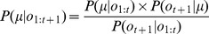
Figure 1. POMP Framework for Decision Making.

Left: The graphical model representing the probabilistic relationship between random variables , , and . In the POMDP model, the hidden state corresponds to coherence and direction jointly. The observation corresponds to MT response . The relations between these variables are summarized in table 1. Right: In order to solve a POMDP problem, the animal maintains a belief , which is a posterior probability distribution over hidden states of the world given observations . At a current belief state , an action is selected according to the learned policy , which maps belief states to actions.

Random dots task as a POMDP

We now describe how the general framework of POMDPs can be applied to the random dots motion discrimination task as shown in Figure 1. In each trial, experimenter chooses a fixed direction corresponding to leftward and rightward motion respectively, and a stimulus strength (motion coherence) , where corresponds to completely random motion and corresponds to coherent motion (i.e., all dots moving in the same direction). Intermediate values of represent a corresponding fraction of dots moving in the coherent direction (e.g., represents coherent motion). The animal is shown a movie of randomly moving dots, a fraction of which are moving in the same direction .

In a given trial, neither the direction nor the coherence is known to the animal. We therefore regard as the joint hidden environment state in the POMDP model. Neurophysiological evidence suggests that information regarding random dot motion is received from neurons in cortical area MT [18]–[21]. Therefore, following previous models (e.g., [22]–[24]), we define the observation model in the POMDP as a function of the responses of MT neurons. Let the firing rate of MT neurons preferring rightward and leftward direction be and respectively. We can define:

(1)

where spikes/second is the average spike rate for coherent motion stimulus, and and are the “drive” in the preferred and null directions respectively. These constants (, and ) are based on fits to experimental data as reported in [23], [25]. Let be the elapsed time between time steps and . Then, the number of spikes emitted by MT neurons within follows a Poisson distribution:

(2)

We define the observation at time as the spike count from MT neurons preferring rightward motion, given the total spike count from rightward and leftward-preferring neurons, i.e., the observation is a conditional random variable where . Then follows a stationary Binomial distribution . Note that the duration of each POMDP time step need not be fixed, and we can therefore adjust such that for some fixed , i.e., the animal updates the posterior distribution over hidden state each time it receives spikes from the MT population. is exponentially distributed, and the standard deviation of will approach zero as increases. When , becomes an indicator random variable representing whether a spike was emitted by a rightward motion preferring neuron or not.

It can be shown [26] that follows a Binomial distribution with

(3)

represents the probability that the MT neurons favoring rightward movement will spike given that there is a spike in the MT population. Since is a joint function of and , we could equivalently regard it as the hidden state of our POMDP model: indicates rightward direction () while indicates the opposite direction (). The coherence corresponds to while corresponds to the two extreme values or for direction being left or right respectively. Note that both direction and coherence are unknown to the animal in the experiments, but they are held constant within a trial.

Bayesian inference of hidden state

Given the framework above, the task of deciding the direction of motion of the coherently moving dots is equivalent to the task of deciding whether or not, and deciding when to make such a decision. The POMDP model makes decisions based on the “belief” state , which is the posterior probability distribution over given a sequence of observations :

(4)

where 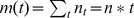, , and 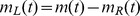. To facilitate the analysis, we represent the prior probability as a beta distribution with parameters and . Note that the beta distribution is quite flexible: for example, a uniform prior can be obtained using . Without loss of generality, we will fix throughout this paper. The posterior distribution can now be written as:

(5)

The belief state at time step thus follows a beta distribution with two parameters and as defined above. Consequently, the posterior probability distribution over depends only on the number of spikes and for rightward and leftward motion respectively. These in turn determine and , where

(6)

is the point estimator of , and . The animal only needs to keep track of and in order to encode the belief state . After marginalizing over coherence , we have the posterior probability over direction :

(7)

(8)

where 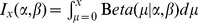is the regularized incomplete beta function.

Actions, rewards, and value function

The animal updates its belief after receiving the current observation , and chooses one of the three actions (decisions) , denoting rightward eye movement, leftward eye movement, and sampling (i.e., waiting for one more observation) respectively. The model assumes the animal receives rewards as follows (rewards are modeled using real numbers). When the animal makes a correct choice, , a rightward eye movement when () or a leftward eye movement when (), the animal receives a positive reward . The animal receives a negative reward (i.e., penalty) or nothing when an incorrect action is chosen . We further assume that the animal is motivated by hunger or thirst to make a decision as quickly as possible. This is modeled using a unit penalty for each observation the animal makes, representing the cost the animal needs to pay when choosing the sampling action .

Recall that a belief state is determined by the parameters . The goal of the animal is to find an optimal “policy” that maximizes the “value” function , defined as the expected sum of future rewards given the current belief state:

(9)

where the expectation is taken with respect to all future belief states 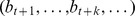. The reward term above is the expected reward for the given belief state and action:

(10)

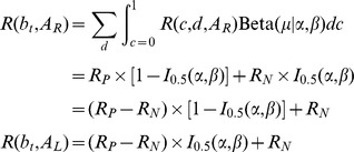The above equations can be interpreted as follows. When is selected, the animal receives more samples at a cost of . When is selected, the expected reward depends on the probability density function of the hidden parameter given belief state . With probability , the true parameter is less than , making an incorrect decision with penalty , and with probability , action is correct, earning the reward .

Finding the optimal policy

A policy defines a mapping from a belief state to one of the available actions . A method for learning a POMDP policy by trial and error using the method of temporal difference (TD) learning was suggested in [11]. Here, we derive a policy from first principles and compare the result with behavioral data.

One standard way [12] to solve a POMDP is to first convert it into a Markov Decision Process (MDP) over belief state, and then apply standard dynamical programming techniques such as value iteration [27] to compute the value function in equation 9. For the corresponding belief MDP, we need to define the transition probabilities 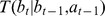. When , the belief state can be updated using the previous belief state and current observation based on Bayes' rule:

(11)

for all . In the above equation, is the Kronecker delta, and is the expected value of the likelihood function over the posterior distribution :

(12)

which is a stationary distribution independent of time . When the selected action is or , the animal stops sampling and makes an eye movement. To account for such cases, we include an additional state , representing a terminal state, with zero reward and absorbing behavior, for all actions . Formally, the transition probabilities with respect to the absorbing (termination) state are defined as for all , indicating the end of a trial.

Given the time-independent belief state transition , the optimal value and policy can be obtained by solving Bellman's equation:

(13)

Before we proceed to results from the model, we note that the one-step belief transition probability matrix with can be shown be mathematically equivalent to the -steps transition matrix with . The solution to Bellman's equation 13 is independent of . Therefore, unless otherwise mentioned, the results are based on the most general scenario where the animal needs to select an action whenever a new spike is received, , .

We summarize the model variables as well as their statistical relationships in table 1.

Table 1. Summary of model variables and paramters.

POMDP Variables	Descriptions
	The hidden variable of POMDP, . In the random dots task, is a constant over time
	The coherence (motion strength) of the random dots task. . is fixed during a task.
	The underlying direction of the random dots task. . is fixed during a task.
	The average spike rate of MT neurons preferring rightward or leftward direction, respectively, as a function of both coherence and described in equations 1.
	The number of spikes emitted by MT neurons preferring rightward or leftward direction, respectively during one POMDP step. follows a Poisson distribution with mean
	Total number of spikes emitted by MT neurons during one POMDP step.
	The noisy observation at time step t, which is a conditional random variable following a Binomial distribution . Note that are conditional dependent of each other given the hidden variable
	The belief (posterior distribution) . With a beta-distributed initial belief , is also beta distributed due to the binomial distributed emission probability . Without loss of generality, throughout the paper.
	Action chosen by the animal at time . .
Model Parameters
	A negative reward associated with the cost of an observation.
	A positive reward associated with a correct eye movement.
	A negative reward associated with an incorrect eye movement.
	The duration of a single observation, the real elapsed time per POMDP step. Only used to translate the number of POMDP time steps to real elapsed time when comparing with experimental data.
	Non-decision residual time. Both and are obtained from a linear regression to compare model predictions (in unit of POMDP steps) with animals' response time (in unit of seconds), independent of the POMDP model.

Results

Optimal value function and policy

Figure 2 (a) shows the optimal value function computed by applying value iteration [27] to the POMDP defined in the Methods and Analysis section, with parameters , , and . The -axis of Figure 2 (a) represents the total number of observations encountered thus far, which is equal to the elapsed time in the trial. The -axis represents the ratio , which is the estimator of the hidden parameter . In general, the model predicts a high value when is close to or , or equivalently, when the estimated coherence is close to . This is because at these two extremes, selecting the appropriate action has a high probability of receiving a large positive reward . On the other hand, for near (estimated near ), choosing or in these states has a high chance of resulting in an incorrect decision and a large negative reward (see [11] for a similar result using a different model and under the assumption of a deadline). Thus, belief states with have a much lower value compared to belief states with or .

Figure 2. Optimal Value and Policy for the Random Dots Task.

(a) Optimal value as a joint function of 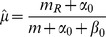and the number of POMDP steps . (b) Optimal Policy as a function of and the number of POMDP steps . The boundaries and divide the belief space into three areas: (red), (green), and (blue), each of which represents belief states whose optimal actions are and respectively. Model parameters: , , and . (c) Left: The rightward decision boundary for different values of . Right: The half time of for different values of , where .

Figure 2 (b) shows the corresponding optimal policy as a joint function of and . The optimal policy partitions the belief space into three regions: , , and , representing the set of belief states preferring actions , and respectively. Let be the set of belief states preferring action after observations, for and . Early in a trial, when is small, the model selects the sampling action regardless of the value of . This is because for small , the variance of the point estimator is high. For example, even when when , the probability that the true is still high. The sampling action is required to reduce this variance by accruing more evidence. As becomes larger, the variance of decreases, and the deviation between and the true value of diminishes by the law of large numbers. Consequently, the animal will pick action even when is only slightly above . This gradual decrease in the threshold over time for choosing the overt actions or has been called a “collapsing bound” in the decision making literature [28]–[30].

The optimal policy is entirely determined by three reward parameters . At a given belief state, picks one of the three available actions that leads to the largest expected future reward. Thus, the choice is determined by the relative, not the absolute, value of the expected future reward for the different actions. From equation 10, we have

(14)

If we regard the sampling penalty as specifying the unit of reward, the optimal policy is determined by the ratio alone. Figure 2 (c) shows the relationship between and the optimal policy by showing the rightward decision boundaries for different values of . As increases (e.g., by making the sampling cost smaller), the boundary gradually moves towards the upper right corner, giving the animal more time to make decisions which results in more accurate decisions. To better understand this relationship, we fit the decision boundary to a hyperbolic function:

(15)

We find that exhibits nearly logarithmic growth with . Interestingly, a collapsing bound is obtained even with extremely small because the goal is reward maximization across trials: it is better to terminate a trial and accrue reward in future trials than to continue sampling noisy (possibly coherent) stimuli.

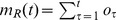
Model predictions: psychometric function and reaction time

We compare predictions of the model based on the learned policy with experimental data from the reaction time version (rather than the fixed duration version) of the motion discrimination task [31]. As illustrated in Figure 3, the model assumes that motion information regarding the random dots on the screen is processed by MT neurons. These neurons provide the observations (and ) to right- and left-direction coding LIP neurons, which maintain the belief state . Actions are selected based on the optimal policy . If or , the animal makes a rightward or leftward decision respectively and terminates the trial. When , the animal chooses the sampling action and gets a new observation .

Figure 3. Relationship between Model and Neural Activity.

The input to the model is a random dots motion sequence. Neurons in MT with tuning curves emit spikes at time step , which constitutes the observation in the POMDP model. The animal maintains the belief state by computing ( can be parameterized by and - see text). The optimal policy is implemented by selecting rightward eye movement when , or equivalently, when (and likewise for leftward eye movement ).

The performance on the task using the optimal policy can be measured in terms of both the accuracy of direction discrimination (the so-called psychometric function), and the reaction time required to reach a decision (the chronometric function). In this section, we derive the expected accuracy and reaction time as a function of stimulus coherence , and compare them to the psychometric and chronometric functions of a monkey performing the same task [31].

The sequence of random variables forms a (non-stationary) Markov chain with transition probabilities determined by equation 11. Let be the joint probability that the animal keeps selecting until time step :

(16)

At , the animal will select regardless of under , making . At , can be expressed recursively as:

(17)

Let and be the joint probability mass functions that the animal makes a right or left choice at time , respectively. These correspond to the probability that the point estimator crosses the boundary of or for the first time at time :

(18)

(19)

The probabilities of making rightward or leftward eye movement are the marginal probabilities summing over all possible crossing times: 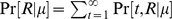and . When the underlying motion direction is rightward, represents the accuracy of motion discrimination and represents the error rate. The mean reaction times for correct and error choices are the expected crossing times over the conditional probability that the animal makes decision and respectively at time :

(20)

(21)

The left panel of Figure 4 shows performance accuracy as a function of motion strength for the model (solid curve) and a monkey (black dots). The model parameters are the same as those in Figure 2, obtained using a binary search within with a minimum step size .

Figure 4. Comparison of Performance of the Model and Monkey.

Black dots with error bars represent a monkey's decision accuracy and reaction time for correct trials. Blue solid curves are model predictions ( and in the text) for parameter values 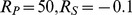, and . Monkey data from [31].

The right panel of Figure 4 shows for the same model parameters the predicted mean reacton time for correct choices as a function of coherence (and fixed direction ) for the model (solid curve) and the monkey (black dots). Note that represents the expected number of POMDP time steps for making a rightward eye movement . It follows from the Poisson spiking process that the duration of each POMDP time step follows a exponential distribution with its expectation proportional to . In order to make a direct comparison to the monkey data , which is in units of real time, a linear regression was used to to determine the duration of a single observation and the onset of decision time :

(22)

Note that the reaction time in a trial is the sum of decision time plus the non-decision delays whose properties are not well understood. The offset represents the non-decision residual time. We applied the experimental mean reaction time reported in [31] with motion coherence to compute the two coefficients and . The unit duration per POMDP step ms/step, and the offset ms, which is comparable to the ms non-decision time on average reported in the literature [23], [32].

There is essentially one parameter in our model needed to fit the experimental accuracy data, namely, the reward ratio . The other two parameters and are independent of the POMDP model, and are used only to translate the POMDP time steps into real elapsed time. This reward ratio has direct physical interpretation and can be easily manipulated by the experimenters. For example, changing the amount of awards for the correct/incorrect choices, or giving subjects different speed instructions will effectively change . In Figure 5 (a), we show performance accuracies and predicted mean reaction time with different values of . With fixed and , decreasing makes the observations more affordable and allows subjects to accumulate more evidence, in turn leads to a longer decision time and higher accuracy. Our model thus provides a quantitative framework for predicting the effects of reward parameters on the accuracy and speed of decision making. To test our theory, we compare the model predictions with the experimental data from a human subject, reported by Hanks et al [33], under different speed-accuracy regimes. In their experiments, human subjects were instructed to perform the random dots task under different speed-accuracy conditions. The red crosses in Figure 5 (b) represent the response time and accuracy of a human subject in the direction discrimination task with instructions to perform the task more carefully at a slower speed, while the black dots represent the task under normal speed conditions. The slower speed instruction encourages human subjects to accumulate more observations before making the final decision. In the model, this amounts to reducing the negative cost associated with each sample . Indeed, this tradeoff between speed and accuracy was consistent with predicted effects of changing the reward ratio. We first fit the model parameters to experimental data under normal speed conditions, based on fitting , ms/step, and ms (Figure 5 (b), black solid curves). The red dashed lines shown in Figure 5 (b) are model fits to the data under slower speed instruction. There is just one degree of freedom in this fit, as all model parameters except the reward ratio were fixed to the values used to fit data in the normal speed regime.

Figure 5. Effect of on speed-accuracy tradeoff.

(a) Model predictions of psychometric and chronometric functions for different values of . (b) Comparison of model predictions and experimental data for different speed-accuracy regimes. The black dots represent the response time and accuracy of a human subject in the direction discrimination task under normal speed conditions, while the red crosses represent data with a slower speed instruction. The model predictions are plotted as black solid curves (with 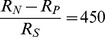) and red dashed lines (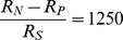), respectively. The per-step duration and non-decision residual time are fixed to be the same for both conditions: ms/step, and ms. Human data are from human subject LH in [33].

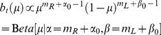
Neural response during direction discrimination task

From Figure 2 (b), it is clear that for the random dots task, the animal does not need to store the whole two dimensional optimal policy but only the two one-dimensional decision boundaries and . This naturally suggests a neural mechanism for decision making similar to that in drift diffusion models: LIP neurons compute the belief state from MT responses and employ divisive normalization to maintain the point estimate . We now explore the hypothesis that the response of LIP neurons represents the difference between and the optimal decision threshold . In this model, a rightward eye movement is initiated only when the difference reaches a fixed bound (in this case, ). Therefore, we modeled the firing rates in the lateral intraparietal area (LIP) as:

(23)

where is the spontaneous firing rate for LIP neurons. Since , a constant is added to make . represents the termination bound; spikes s from [30]. The firing rate is defined similarly.

The above model makes two testable predictions about neural responses in LIP. The first is that the neural response to coherent motion (the so called “urgency” signal [30], [34]) encodes the decision boundary (or for leftward-preferring LIP neurons). In Figure 6a, we plot the model response to coherent motion, along with a fit to a hyperbolic function , the same function that Churchland et al [30] used to parametrize the experimentally observed “urgency signal.” The parameter is the time taken to reach of the maximum. The estimate of for the model from Figure 6 (a) is ms, which is consistent with the ms estimated from neural data [30].

Figure 6. Comparison of Model and Neural Responses.

(a) Model response to coherence motion is shown in red. Blue curve depicts a fit using a hyperbolic function where ms, which is comparable to the value of ms estimated from neural data [30]. (b) The first ms of decision time was used to compute the buildup rate from the model response following the procedure in [30]. The red points show model buildup rates estimated for each coherence value. The effect of a unit change in the coherence on buildup rate can be estimated from the slope of the blue fitted line: this value, spike s coh, is similar to the corresponding value spike s coh estimated from neural data [30].

The second prediction concerns the buildup rate (in units of spikes s coh) of the LIP firing rates. The buildup rate of LIP at each motion strength is calculated from the slope of a line fit to model LIP firing rate during the first ms of decision time. As shown in Figure 6 (b), buildup rates scaled approximately linearly as a function of motion coherence. The effect of a unit change in coherence on the buildup rate can be estimated from the slope of the fitted line to be spike s coh, similar to what has been reported in the literature [30] ( spike s coh).

Discussion

The random dots motion discrimination task has provided a wealth of information regarding decision making in the primate brain. Much of this data has previously been modeled using the drift diffusion model [35], [36], but to fully account for the experimental data, one has to sometimes use ad-hoc assumptions. This paper introduces an alternative model for explaining the monkey's behavior based on the framework of partially observable Markov decision processes (POMDPs).

We believe that the POMDP model provides a more versatile framework for decision making compared to the drift diffusion model, which can be viewed as a special case of sequential statistical hypothesis testing (SSHT) [37]. Sequential statistical hypothesis testing assumes that the stimuli (observations) are independent and identically distributed whereas the POMDP model allows observations be temporally correlated. The observations in the POMDP are conditionally independent given the hidden state , which evolves according to a Markov chain. Thus, the POMDP framework for decision making [11], [14], [16], [38], [39] can be regarded as a strictly more general model than the SSHT models. We intend to explore the applicability of our POMDP model to time-dependent stimuli, such as temporally dynamic attention [40] and temporally blurred stimulus representations [41] in future studies.

Another advantage of a POMDP model is that the model parameters have direct physical interpretations and can be easily manipulated by the experimenter. Our analysis shows that the optimal policy is fully determined by the reward parameters . Thus, the model psychometric and chronometric functions, which are derived from the optimal policy, are also fully determined by these model parameters. Experimenters can control these reward parameters by changing the amount of awards for the correct/incorrect choices, or by giving subjects different speed instructions. This allows our model to make testable predictions, as demonstrated by the effects of the change in the reward ratios on the speed-accuracy trade-off. It should be noted that these reward parameters can be subjective and may vary from individual to individual. For example, can be directly related to the external food or juice reward provided by the experimenter while may be linked to internal factors such as degree of hunger or thirst, drive, and motivation. The precise relationship between these reward parameters and the external reward/risk controlled by the experimenter remains unknown. Our model thus provides a quantitative framework for studying this relationship between internal reward mechanisms and external physical reward.

The proposed model demonstrates how the monkey's choices in the random dots task can be interpreted as being optimal under the hypothesis of reward maximization. The reward maximization hypothesis has previously been used to explain behavioral data from conditioning experiments [8] and dopaminergic responses under the framework of temporal difference (TD) learning [42]. Our model extends these results to the more general problem of decision making under uncertainty. The model predicts psychometric and chronometric functions that are quantitatively close to those observed in monkeys and humans solving the random dots task.

We showed through analytical derivations and numerical simulation that the optimal threshold for selecting overt actions is a declining function of time. Such a collapsing decision bound has previously been obtained for decision making under a deadline [11], [29]. It has also been proposed as an ad-hoc mechanism in drift diffusion models [28], [30], [43] for explaining finite response time at zero percent coherence. Our results demonstrate that a collapsing bound emerges naturally as a consequence of reward maximization. Additionally, the POMDP model readily generalizes to the case of decision making with arbitrary numbers of states and actions, as well as time-varying state.

Instead of traditional dynamic programming techniques, the optimal policy and value can be learned via Monte Carlo approximation-based methods such as temporal difference (TD) learning [27]. There is much evidence suggesting that the firing rate of midbrain dopaminergic neurons might represent the reward prediction error in TD learning. Thus, the learning of value and policy in the current model could potentially be implemented in a manner similar to previous TD learning models of the basal ganglia [8], [9], [11], [42].

Funding Statement

This project was supported by the National Science Foundation (NSF) Center for Sensorimotor Neural Engineering (EEC-1028725), NSF grant 0930908, Army Research Office (ARO) award W911NF-11-1-0307, and Office of Naval Research (ONR) grant N000140910097. YH is a Howard Hughes Medical Institute International Student Research fellow. The funders had no role in study design, data collection and analysis, decision to publish, or preparation of the manuscript.

References

- 1.Knill D, Richards W (1996) Perception as Bayesian inference. Cambridge: Cambridge University Press.
- 2. Zemel RS, Dayan P, Pouget A (1998) Probabilistic interpretation of population codes. Neural Computation 10. [DOI] [PubMed] [Google Scholar]
- 3.Rao RPN, Olshausen BA, Lewicki MS (2002) Probabilistic Models of the Brain: Perception and Neural Function. Cambridge, MA: MIT Press.
- 4. Rao RPN (2004) Bayesian computation in recurrent neural circuits. Neural Computation 16: 1–38. [DOI] [PubMed] [Google Scholar]
- 5. Ma WJ, Beck JM, Latham PE, Pouget A (2006) Bayesian inference with probabilistic population codes. Nature Neuroscience 9: 1432–1438. [DOI] [PubMed] [Google Scholar]
- 6.Doya K, Ishii S, Pouget A, Rao RPN (2007) Bayesian Brain: Probabilistic Approaches to Neural Coding. Cambridge, MA: MIT Press.
- 7. Daw ND, Courville AC, Touretzky D (2006) Representation and timing in theories of the dopamine system. Neural Computation 18: 1637–1677. [DOI] [PubMed] [Google Scholar]
- 8. Dayan P, Daw ND (2008) Decision theory, reinforcement learning, and the brain. Cognitive, Affective and Behavioral Neuroscience 8: 429–453. [DOI] [PubMed] [Google Scholar]
- 9. Bogacz R, Larsen T (2011) Integration of reinforcement learning and optimal decision making theories of the basal ganglia. Neural Computation 23: 817–851. [DOI] [PubMed] [Google Scholar]
- 10. Law CT, Gold JI (2009) Reinforcement learning can account for associative and perceptual learning on a visual-decision task. Nat Neurosci 12: 655–663. [DOI] [PMC free article] [PubMed] [Google Scholar]
- 11. Rao RPN (2010) Decision making under uncertainty: A neural model based on POMDPs. Frontiers in Computational Neuroscience 4. [DOI] [PMC free article] [PubMed] [Google Scholar]
- 12. Kaelbling LP, Littman ML, Cassandra AR (1998) Planning and acting in partially observable stochastic domains. Artificial Intelligence 101: 99–134. [Google Scholar]
- 13. Drugowitsch J, Moreno-Bote R, Churchland AK, Shadlen MN, Pouget A (2012) The cost of accu-mulating evidence in perceptual decision making. J Neurosci 32: 3612–3628. [DOI] [PMC free article] [PubMed] [Google Scholar]
- 14.Shenoy P, Rao RPN, Yu AJ (2010) A rational decision-making framework for inhibitory control. Advances in Neural Information Processing Systems (NIPS) 23. Available: http://www.cogsci.ucsd.edu/~ajyu/Papers/nips10.pdf. Accessed 2012 Dec 24.
- 15.Shenoy P, Yu AJ (2012) Rational impatience in perceptual decision-making: a bayesian account of discrepancy between two-alternative forced choice and go/nogo behavior. Advances in Neural Information Processing Systems (NIPS) 25. Cambridge, MA: MIT Press.
- 16.Huang Y, Friesen AL, Hanks TD, Shadlen MN, Rao RPN (2012) How prior probability influences decision making: A unifying probabilistic model. Advances in Neural Information Processing Systems (NIPS) 25. Cambridge, MA: MIT Press.
- 17. Shadlen MN, Newsome WT (2001) Neural basis of a perceptual decision in the parietal cortex (area LIP) of the rhesus monkey. Journal of Neurophysiology 86. [DOI] [PubMed] [Google Scholar]
- 18. Newsome WT, Britten KH, Movshon JA (1989) Neuronal correlates of a perceptual decision. Nature 341: 52–54. [DOI] [PubMed] [Google Scholar]
- 19. Salzman CD, Britten KH, Newsome WT (1990) Cortical microstimulation inuences perceptual judgements of motion direction. Nature 346: 174–177. [DOI] [PubMed] [Google Scholar]
- 20. Britten KH, Shadlen MN, Newsome WT, Movshon JA (1992) The analysis of visual motion: a comparison of neuronal and psychophysical performance. J Neurosci 12: 4745–4765. [DOI] [PMC free article] [PubMed] [Google Scholar]
- 21. Shadlen MN, Newsome WT (1996) Motion perception: seeing and deciding. Proc Natl Acad Sci 93: 628–633. [DOI] [PMC free article] [PubMed] [Google Scholar]
- 22. Wang XJ (2002) Probabilistic decision making by slow reverberation in cortical circuits. Neuron 36: 955–968. [DOI] [PubMed] [Google Scholar]
- 23. Mazurek ME, Roitman JD, Ditterich J, Shadlen MN (2003) A role for neural integrators in per-ceptual decision-making. Cerebral Cortex 13: 1257–1269. [DOI] [PubMed] [Google Scholar]
- 24. Beck JM, Ma W, Kiani R, Hanks TD, Churchland AK, et al. (2008) Probabilistic population codes for Bayesian decision making. Neuron 60: 1142–1145. [DOI] [PMC free article] [PubMed] [Google Scholar]
- 25. Britten KH, Shadlen MN, Newsome WT, Movshon JA (1993) Responses of neurons in macaque MT to stochastic motion signals. Vis Neurosci 10(6): 1157–1169. [DOI] [PubMed] [Google Scholar]
- 26.Casella G, Berger R (2001) Statistical Inference, 2nd edition. Pacific Grove, CA: Duxbury Press.
- 27.Sutton RS, Barto AG (1998) Reinforcement Learning: An Introduction. Cambridge, MA: MIT Press.
- 28. Latham PE, Roudi Y, Ahmadi M, Pouget A (2007) Deciding when to decide. SocNeurosciAbstracts 740. [Google Scholar]
- 29. Frazier P, Yu A (2008) Sequential hypothesis testing under stochastic deadlines. Advances in Neural Information Processing Systems 20: 465–472. [Google Scholar]
- 30. Churchland AK, Kiani R, Shadlen MN (2008) Decision-making with multiple alternatives. Nat Neurosci 11: 693–702. [DOI] [PMC free article] [PubMed] [Google Scholar]
- 31. Roitman JD, Shadlen MN (2002) Response of neurons in the lateral intraparietal area during a combined visual discrimination reaction time task. Journal of Neuroscience 22 21: 9475–9489. [DOI] [PMC free article] [PubMed] [Google Scholar]
- 32.Luce RD (1986) Response times: their role in inferring elementary mental organization. Oxford: Oxford University Press.
- 33. Hanks TD, Mazurek ME, Kiani R, Hopp E, Shadlen MN (2011) Elapsed decision time affects the weighting of prior probability in a perceptual decision task. Journal of Neuroscience 31: 6339–6352. [DOI] [PMC free article] [PubMed] [Google Scholar]
- 34. Cisek P, Puskas G, El-Murr S (2009) Decisions in changing conditions: The urgency-gating model. Journal of Neuroscience 29: 11560–11571. [DOI] [PMC free article] [PubMed] [Google Scholar]
- 35. Palmer J, Huk AC, Shadlen MN (2005) The effects of stimulus strength on the speed and accuracy of a perceptual decision. Journal of Vision 5: 376–404. [DOI] [PubMed] [Google Scholar]
- 36. Bogacz R, Brown E, Moehlis J, Hu P, Holmes P, et al. (2006) The physics of optimal decision making: A formal analysis of models of performance in two-alternative forced choice tasks. Psychological Review 113: 700–765. [DOI] [PubMed] [Google Scholar]
- 37. Lai TL (1988) Nearly optimal sequential tests of composite hypotheses. The Annals of Statistics 16 2: 856–886. [Google Scholar]
- 38.Frazier PL, Yu AJ (2007) Sequential hypothesis testing under stochastic deadlines. In Advances in Neural Information procession Systems 20. Cambridge, MA: MIT Press.
- 39. Yu A, Cohen J (2008) Sequential effects: Superstition or rational behavior. In Advances in Neural Information Processing Systems 21: 1873–1880. [PMC free article] [PubMed] [Google Scholar]
- 40. Ghose GM, Maunsell JHR (2002) Attentional modulation in visual cortex depends on task timing. Nature 419 6907: 616–620. [DOI] [PubMed] [Google Scholar]
- 41. Ludwig CJH (2009) Temporal integration of sensory evidence for saccade target selection. Vision Research 49: 2764–2773. [DOI] [PubMed] [Google Scholar]
- 42. Schultz W, Dayan P, Montague PR (1997) A neural substrate of prediction and reward. Science 275: 1593–1599. [DOI] [PubMed] [Google Scholar]
- 43. Ditterich J (2006) Stochastic models and decisions about motion direction: Behavior and physiology. Neural Networks 19: 981–1012. [DOI] [PubMed] [Google Scholar]