Haustral Fold Segmentation with Curvature-Guided Level Set Evolution

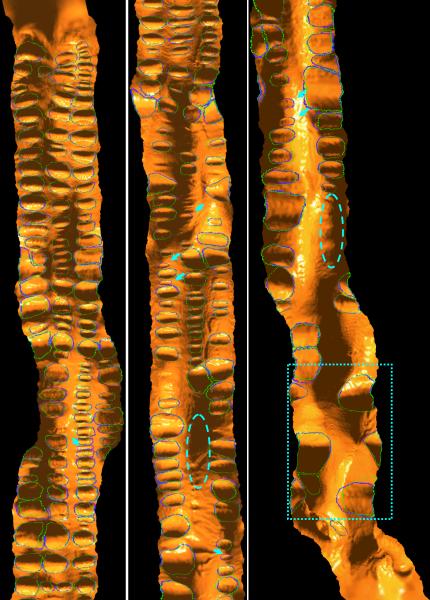
Abstract

Human colon has complex structures mostly because of the haustral folds. The folds are thin flat protrusions on the colon wall, which complicate the shape analysis for computer-aided detection (CAD) of colonic polyps. Fold segmentation may help reduce the structural complexity, and the folds can serve as anatomic reference for computed tomographic colonography (CTC). Therefore, in this study, based on a model of the haustral fold boundaries, we developed a level-set approach to automatically segment the fold surfaces. To evaluate the developed fold segmentation algorithm, we first established the ground truth of haustral fold boundaries by experts' drawing on 15 patient CTC datasets without severe under/over colon distention from two medical centers. The segmentation algorithm successfully detected 92.7% of the folds in the ground truth. In addition to the sensitivity measure, we further developed a merit of segmented area ratio (SAR), i.e., the ratio between the area of the intersection and union of the expert-drawn folds and the area of the automatically-segmented folds, to measure the segmentation accuracy. The segmentation algorithm reached an average value of SAR=86.2%, showing a good match with the ground truth on the fold surfaces. We believe the automatically-segmented fold surfaces have the potential to benefit many post-procedures in CTC, such as CAD, taenia coli extraction, supine-prone registration, etc.

I. Introduction

According to the recent statistics from American Cancer Society (ACS) [1], colorectal cancer ranks the third most common occurrence of both cancer deaths and new cancer cases for both men and women in the United States. Computer-aided detection (CAD) of colonic polyps (CRPs, precursors of colon cancers), is known as a promising second reader [2–3] for computed tomographic colongraphy (CTC) [4]. However, existing CAD schemes have being scolded for the impractical detection sensitivity for non-polypoid [5] and small (less than 10 mm) [6] CRPs. In existing CAD schemes, mathematical filters responsive to the morphological characteristics of CRPs such as the round-tip feature, are used to search for CRPs [7–8]. These filters are designed by merely modeling the CRPs alone, but seldomly or never considering the environment where the CRPs live in. Unfortunately, the environment of the colon is extremely complex, as shown in Figure 1(a) and 1(b). On the other hand, the above challenging CRPs feature as small shape-changes, which may be “occluded” or “overwhelmed” by the structural complexity of colon [9]. Straightforwardly, a simplified colon representation would be expected to reduce the complexity. Typically, three major sub-structures that form the colon inner wall (colon wall for simplicity) are haustral folds (folds for simplicity), haustrals, and taenia coli (TC) (Figure 1(c)). The idea of colon decomposition shown by the process from Figure 1(c) to 1(d), may provide such simplified representation, where the colon wall would be represented as the haustrals and two sides of folds (Figure 1(d)). These sub-structures are flat and simple. As a result, the conspicuity of the challenging CRPs could be enhanced. To validate such idea, a solid fold segmentation algorithm has to be laid down first, which is the topic of this study.

Figure 1.

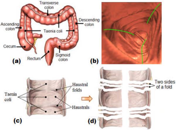
(a) Viewing from outside, the colon is a long tubular structure, but it turns, twists and even mobiles in human abdomen. (b) Viewing from inside, there is a large number of folds extending into the colon lumen, andbetween the folds there are concave haustrals. Three taenia coli (TC, green curves) pass through the folds and haustrals in the longitudinal direction. (c) Three major sub-structures, folds, haustrals and TC. (d) Cutting along the TC, fold peaks and fold boundaries, the colon can be decomposed into pieces representing the haustrals, and the two sides of folds.

In addition, effective segmentation (or quantification) of the folds is significant for detecting polyps on the folds [10]. Moreover, in between the circumferential folds, there are three TC. Segmentation of the folds is also significant for TC extraction [11–14] and supine-prone registration [15–19].

Conceptually, most previous methods in the field mainly focused on fold detection, rather than fold segmentation. For example, in [11–13], folds were detected by thresholding the curvatures in three-dimensional (3D) colon representation, while in [20], the detection task was conducted using a Gabor filter on a 2D unfolded colon representation. In all the above methods, the fold detections did not have evaluation, and the detected folds just served as a reference for TC extraction. Some previous studies were conducted more or less for detecting and segmenting the folds. For example, in [21], initial folds were detected by applying a closing operation on colon lumen image, and then the real folds' extensions were estimated by analyzing the local CT density features. In [22], a heat-diffusion equation was applied to colon lumen image and then a fuzzy C-means strategy was employed to create the initial folds. Some parts of the initial folds were selected as seeds for the input of a level set (LS) method, and the LS method evolved to estimate the extensions of the real folds. In these studies, the focus was on detecting the fold peaks, while little attention was paid to model the fold boundaries for fold segmentation, where the term “fold boundary” indicates the intersecting border on the colon wall between the fold and haustral. Initial effort to model such boundaries as negative ridges was reported in [23], where the fold segmentation was performed by a ridge line detection method. Because of the lack of ground truth, all the above studies reported their performance by just measuring the sensitivity (how many folds per dataset had been found). Therefore, the outcome of these studies conceptually falls into the category of fold detection, despite the fold boundary modeling effort in [23]. In this study, we further explored the initial idea in [23] and presented a model for the colonic folds. Because of its ability of describing the topology of the modeled fold boundaries, the LS method was adapted to segment the colonic folds. To evaluate the segmentation, ground truth was established from 15 patient scans by experts' drawing of the fold boundaries.

The remainder is organized as follows. In Section II, the fold model is described first and then the segmentation method is presented. In Section III, the evaluation design is outlined, which includes the establishment of the ground-truth and the merits for performance measures. The experimental results are reported in Section IV. Finally, some conclusions are drawn following some discussions in Section V.

II. Method

A. Characteristics of folds

Typical folds are thin elongated structures. As shown in Figure 2(a), the fold protrudes from the flat colon wall (haustrals) into the colon lumen. Generally, as seen in Figure 2(a), the surface bends concavely around the blue curves where the fold meets the flat haustral, and bends convexly around the red curve at the top of the fold. Mathematically, such concave/convex bends can be modeled as negative/positive ridges with third-order derivatives [24]. However, the fold ends, as circled by magenta color, often smoothly merge into haustrals, where there are no ridges but umbilics with equal principal curvatures. By definition, the concave bends and the fold ends form the complete boundary of the fold. In [23], we tried to segment the fold by firstly extracting the concave bends as negative ridges and then connecting them near the fold ends. Unfortunately, the high order derivatives are extremely sensitive to noise and tiny shape changes, which lead to lousy and fragmented ridge lines on the colon wall surface, as shown in Figure 2(b). It is cumbersome to remove unwanted ridges and get closed fold boundaries. However, the investigation in [23] still conveys us the message that the fold boundary has the local extremalities of the curvature related measures.

Figure 2.

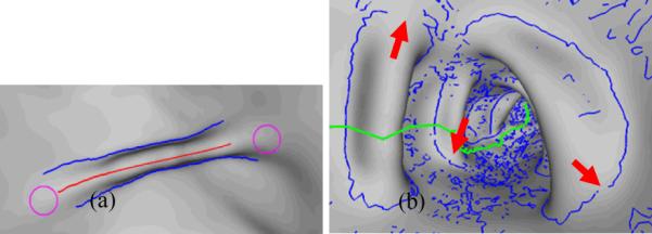
(a) A typical fold. The two blue curves indicate the concave bends where the fold meets its neighboring haustrals. The red curve denotes the convex bend at the top of the fold (fold peak). However, at the two fold ends around the two magenta circles, the fold smoothly merges into the haustral. (b) The blue curves are the detected ridge lines in [23]. Arrows indicate disconnections of the ridge lines at the fold boundaries. The green curve indicates the colon centerline.

Intuitively, the concave bends at fold boundaries have positive κ₁ and κ₂ (the first and second principal curvatures), which lead to local maximal mean curvatures, H = (κ₁ + κ₂) / 2. Such fact can be verified by the circled peaks in Figure 3(c) and 3(d). At the flat fold ends, both κ₁ and κ₂ are approximately constants, which indicates constant mean curvatures. The rectangle in Figure 3(c) demonstrates such area with almost constant H. However, the rectangle in Figure 3(d) contains a small peak because the relative fold end is not flat, and it noticeably bends rather than smoothly merging into the haustral (as seen in Figure 3(b)). Although the concave bends and fold ends show different patterns of H distribution, they still share one common feature that both the local maximal H (at concave bends and bended fold ends) and constant H (at flat fold ends) have diminished gradients. Therefore, we expect that the gradients of H can guide a deformable model, such as the LS method, to extract the complete or closed fold boundary. It should be noted that the deformable model will evolve on the surface rather than in the image volume.

Figure 3.

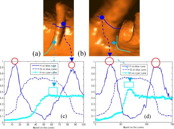
Fold characteristics analysis. (a) A typical fold from descending colon. (b) A thick fold from sigmoid colon. (c) Curvature analysis on the fold in (a). (d) Curvature analysis on the fold in (b). With the software tool (to be detailed in Section III.A), we manually draw paths on the fold surfaces such as the thick curves in (a) and (b). Points are evenly sampled on the curves, and the smoothed shape index and mean curvature are calculated (to be detailed in Section II.C and II.D) and plotted in (c) and (d). For each point, the curvature measure is calculated by interpolation. The curve arrows indicate that the circle/rectangle areas are near to the locations on the 3D curves. Two red circles in (c) and (d) with no arrows represent the concaves on the other sides of the folds. Finally, the mean curvature and shape index are unitized into (0, 1] on the whole colon wall.

To facilitate the deformable model, a seeding area is needed to initiate the iterative LS procedure. For fold segmentation, the fold peaks can be relatively easily detected and are selected as the perfect seeding areas to start the iterative procedure. As mentioned above, the fold peaks are local ridge-like structures. Instead of using the third-order derivatives to detect such ridges [24], the shape index, SI = 1/ 2 − (1/π) arctan $\frac{k_1+k_2}{k_1-k_2}$ which involves only the second order derivatives with better immunity to noise, can also be employed to detect the fold peaks. The ridge-like structures (fold peaks) have large SI, while the “rut” (concave bends) and “saddle” (fold ends) structures have small SI [25]. The central large peaks of the dashed curves in Figure 3(c) and 3(d) illustrate such characteristics of the fold peaks. Therefore, the fold peaks can be extracted by thresholding SI.

B. Overview of segmentation algorithm

Based on the fold characteristics as described above, we adapt the LS method to fulfill the task of fold segmentation. The SI will be used to extract the initial fold area (the fold peak). The boundary of the initial fold area will be used to build up the initial LS function, and H will be employed to guide the LS evolution procedure to retrieve the closed fold boundaries. The whole flowchart for the fold segmentation algorithm is outlined in Figure 4.

Figure 4.

The whole flowchart of the fold segmentation algorithm.

The CTC volume image is first segmented [26, 27], and then the marching cube method [28, 29] is employed to extract the colon wall surface as a triangle mesh representation. These two operations are the pre-processing steps for the presented fold segmentation algorithm (shown by the three solid boxes in Figure 4). Bear in mind that the image resolution is very high [30] and the folds are relatively large objects in the scale of the resolution. Therefore, the extracted colon wall surface has a large size in the triangle mesh representation [29] and so does each fold [23]. This gives us the opportunity to operate on the triangle mesh representation to handle the image noise and other artifacts for fold segmentation. The presented fold segmentation algorithm starts by the operations on the triangle mesh representation of the colon wall surface.

C. Smoothing operation in triangular surface domain

In practice, image noise is not avoidable. The noise could be further amplified by post-image processing operations like curvature (the second-order derivative) estimation. Since the curvature estimation at each vertex of the triangular mesh surface is needed to describe the fold characteristics, noise control then becomes necessary. Therefore, our fold segmentation algorithm starts by smoothing the triangular mesh surface before the curvature estimation. The smoothing operation is also applied to the information generated from the triangular mesh surface.

To help understanding the methodology in this study, we would like to establish some basic concepts in the triangular surface domain. Figure 5(a) defines part of the point area of p₀ (the shadow area). As a result, the sum of contributions from all triangles, sharing the point p₀ on the surface such as the triangles in the 1-ring neighborhood as in Figure 5(b), defines the whole point area of p₀. Based on these concepts, we develop a Gaussian weighted smooth operation

$$\overline{f^{\mathit{info}}}=\frac{\sum _i^{N_r}{w}_i\cdot f_i^{\mathit{info}}}{\sum _i^{N_r}{w}_i},$$ (1)

where f^info denotes the information (to be defined later) to be smoothed. $f_i^{info}$ is the information at point p_i, and $\overline{f_{info}}$ is the smoothed result. N_r defines a neighborhood of the center point p₀, of which each point's distance from p₀ is less than a predefined constant r. Weight w_i at point p_i is defined as

$$w_i=\text{cos}{\alpha }_{i,0}\cdot A_i\cdot \text{exp}(-\frac{d_{i,0}^2}{2{\sigma }^2}),$$ (2)

where α_i,0 represents the angle between the normal vectors at p_i and p₀. A_i denotes the point area of point p_i. The underlying rationale of the two terms can be explained straightforwardly. A large α_i,0 suggests that the two points orient very differently, and p_i contributes less to the smoothing process. A small point area A_i implies that there is a dense point distribution near point p_i, and such distribution makes a small contribution because there are most probably some other close points which may also contribute to the same smoothing process. Similar to general Gaussian functions, d_i,0 denotes the distance between the two points, and σ is the user-specified smoothing scale.

Figure 5.

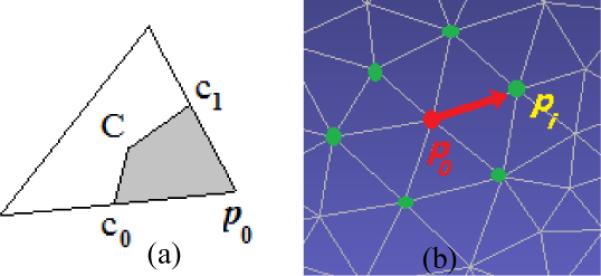
(a) A triangle, the basic element in triangular surface domain. Point C is the barycenter, and c₀, c₁ are the middle points of the edges they are on. Then, the shadow area is part of the point area at p₀ contributed by the triangle. (b) The 1-ring neighborhood, such as the green points p_i with i=1, 2, …, of point p₀ on a triangle mesh, which might be expanded by including more layers of points and refer to as 2-ring, 3-ring, …, neighborhood.

In this study, in addition to smoothing the mesh surface, we also use the scheme to smooth the scalar information, such as H, SI, and the LS function on the colon wall surface. All the smoothing processes are conducted in 2-ring neighborhood with σ = 1.5. In the following text, we focus on the final three parts in the flowchart of Figure 4, which are the curvature analysis, initial fold detection, and LS-based fold segmentation.

D. Curvature analysis on triangle mesh surface

In the theory of differential geometry [31], a local smooth surface can be represented with a bivariate function

$$z=\frac{1}{2}({\kappa }_1{x}^2+{\kappa }_2{y}^2)+h.o.t.,$$ (3)

where (x, y, z) are coordinates of points on the surface in a local orthogonal frame, which is known as Monge coordinate system (MCS). The orthogonal axes of MCS are the first and second principal directions and the normal of the surface at the point. The coefficients κ₁, κ₂ are the two principal curvatures, and h.o.t. denotes high order term. In the local neighborhood of the point (as shown in Figure 5), principal component analysis (PCA) [32] is conducted. Two of the three eigenvectors relating to the two larger eigenvalues can be used to approximate the two principal directions, and the third eigenvector is used as the normal direction. By taking the point as the origin, the MCS of the point can then be established, which can be modeled as a transformation matrix TMCS. By far, with TMCS, we transform the neighborhood to MCS, and the transformed points can be fed into equation (3) to form a inear system. Finally, the principal curvatures κ₁, κ₂ can be estimated by solving the linear system, and accordingly, H and SI can be calculated based on their definitions. Figure 6 shows the smoothed H and SI of a patient scan.

Figure 6.

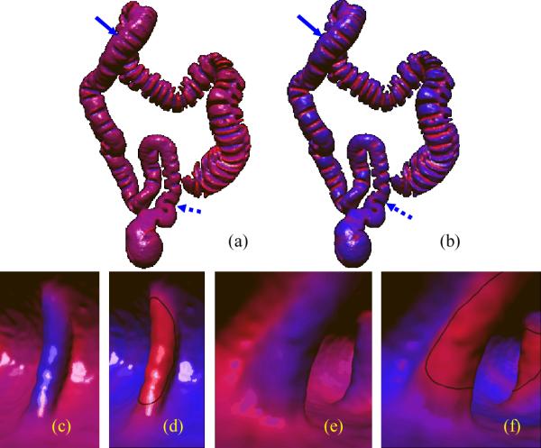
The smoothed mean curvature $\overline{H}$ and shape index $\overline{SI}$ of a patient scan. $\overline{H}$ and $\overline{SI}$ are both unitized into [0, 1], and linearly mapped into colors from blue to red. The mapped colors are displayed directly on the colon surface. (a) $\overline{H}$ on the colon. (b) $\overline{SI}$ on the colon. (c) Close view of $\overline{H}$ on a fold (same fold as in Figure 3(a)). (d) Close view of $\overline{SI}$ on the fold as in (c). (e) Close view of $\overline{H}$ on a fold (same fold as in Figure 3(b)). (f) Close view of $\overline{SI}$ on the fold as in (e). The fold in (c) and (d) is indicated by the solid arrow in (a) and (b), while the fold in (e) and (f) by the dashed arrow. The thick green curves in (d) and (f) indicate the initial fold detections (as detailed in II.E).

E. Initial fold detection

The reddish bands with the local maximum of H, in Figure 6(c) and 6(e) indicate boundaries enclosing the folds, while the red colors in Figure 6(d) and 6(f) denote fold peaks with large SI. These observations verify the fold characteristics analysis as in Figure 3. Therefore, we use the shape index SI to determine the fold peaks as the initial fold detections (to be discussed in the rest of this section), and use the mean curvature H to determine the fold boundaries (to be described in II.F).

E.1. Iso-contour extraction in the surface domain

Analogous to the case of 3D regular image domain, the scalar value like the SI, can be taken as a continuous function, f (v) : S → R, where v is any point on the surface domain S. Accordingly, the curves with a specified constant function value, f (v) = Const., determine the iso-contours on the surface. In this study, the surface domain is discretized by the triangulated mesh, where the iso-contour curves can be extracted using the following algorithm:

• 1)For a triangle, the function values at the three vertices are compared with the specified constant to determine whether the contour intersects with the triangle.
• 2)If there is intersection, points on the triangle edges are linearly interpolated, and connected as a line segment (part of the contour). The line segment is connected to the last line segment if any. The neighbor triangles sharing the intersecting edges of the triangle are taken as new inputs, and go back to (1) until all the triangles on the iso-contour have been processed.
• 3)If there is no intersection, just move to an un-processed triangle of the mesh surface, and go back to (1), until all the triangles have been visited.

In the paper, the iso-contours, $\overline{SI}=0.7$, are extracted as the potential initial fold boundaries (IFBs). Figure 6(d), 6(f), and Figure 7 show examples of the extracted iso-contours. As observed in Figure 7(a) and 7(b), there are some redundant iso-contours induced by non-fold structures like TC or other structures. These redundant iso-contours could be removed by considering the anatomical knowledge of colon folds.

Figure 7.

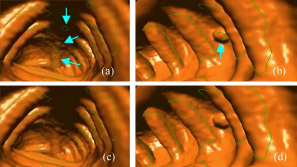
Endoluminal display of the detected iso-contours, i.e., the thick green curves. The arrow-pointed curves are redundant non-fold iso-contours. (a) Redundant iso-contours induced by TC. (b) Redundant iso-contour on a polyp. (c) The IFBs from (a) after filtration. (d) The IFBs from (b) after filtration.

E.2. Filtration of initial fold detections

Human colon is generally a curved tubular object. Three directions, i.e., the longitudinal, radial and circumferential directions, can serve as the references to describe locations inside the colon. Based on the references, folds

• are thin flat with small longitudinal extent, but elongated circumferentially and perpendicular to the colon centerline.

• protrude from the colon wall in the radial direction.

Similar to [23], we model the anatomical feature for each iso-contour. To do that, we turn to PCA analysis once again. Points are evenly sampled on the iso-contour. These points are fed into PCA, and the three eigenvectors represents the three principal directions of the iso-contour. Straightforwardly, the eigenvector, e₀, associated to the largest eigenvalue, indicates the direction with the largest extent of the iso-contour, while the eigenvector, e₂, related to the smallest eigenvalue, denotes the direction with smallest extent (most probably the thickness direction of the fold). As a result, we can design the following features for each iso-contour:

• Axial ratio (AR): AR = (largest extent)/(smallest extent), where the largest/smallest extents can be retrieved by projecting the sampling points onto e₀/e₂. The iso-contours on long narrow true folds give rise to large ARs.

• Centerline-alignment (CA): $CA=\mid \text{cos}\left({\beta }_{e_0,e_c}\right)\mid$, where β_e0,ec represents and the the angle between e₀ and the direction e_c of the associated centerline [33]. For each point on the iso-contour, it associates with a point on the centerline indicating the minimum distance from the ridge point to the centerline. We employ the centerline-based Euclidean distance transform [34] to search for the related points on the centerline, then e_c represents the averaged direction of the tangential directions of the points on the centerline. Intuitively, iso-contours of true folds are often perpendicular to the centerline and lead to small CAs, while non-fold iso-contours like TC induced ones are almost parallel to the centerline and give rise to large CAs.

In this study, iso-contours with AR<2.5 and CA>0.3 are excluded as non-fold detections. Figure 7(c) and 7(d) show the resulted IFBs after such filtration process. These iso-contours are input into the LS framework for fold segmentation.

F. Level set-based fold segmentation

F.1. Concepts

Level set or LS framework is one of the geometric deformable models and is based on the curve evolution theory [35]. Mathematically, let Ω ⊂ R¹ be the data domain, an l-dimensional surface S (the boundary of an open subset ω ∈ Ω, that is, S = ∂ω) is implicitly expressed by a Lipchitz continuous function (the LS function) ϕ (x) : Ω → R, where x = (x₁, x₂,…x_l). The idea is shown in Figure 8 by assuming l = 2. The surface S is the zero-LS surface (ZLSS) of the Lipchitz function where ϕ = 0. Generally, the LS function is given by the signed distance function ϕ = ±d where d is the nearest distance to ZLSS, and ϕ = +d in ω, ϕ = −d in Ω − ω, and ϕ = 0 on ∂ω. For image segmentation, the evolution process of the LS method is described as $\frac{\partial \varphi }{\partial t}+F\Vert \nabla \varphi \Vert =0$ by introducing an artificial time t and force F = F^image + F^geometry. The geometry force, F^geometry, is generated from the LS function itself to control the geometrical and topological properties of the ZLSS during evolution, while the image force, F^image, roots in the image information. By properly defining the edge-based or region-based image forces, LS function evolves and finally terminates its ZLSS on the boundaries of different regions. Practically, the LS function is updated step-by-step as:

$${\varphi }^{(n+1)}-{\varphi }^{\left(n\right)}=-(F^{\mathit{image}}+F^{\mathit{geometry}})\cdot \Delta t\text{with}n\ge 0,$$ (4)

where ϕ⁽ⁿ⁾ is the LS function at the nth time step, and ϕ⁽⁰⁾ the initial LS function when t=0.

Figure 8.

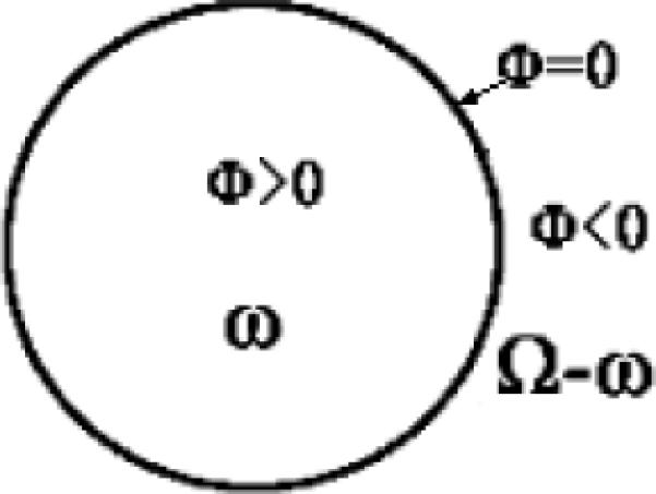
LS function ϕ and ZLSS where ϕ = 0 in the domain Ω.

F.2. Fold segmentation with LS method

The above LS scheme has been widely used for image segmentation in regular 2D or 3D image domain [36, 37]. Interestingly, it can also be extended to irregular domain, like triangulated surface domain [22, 38]. Analogous to the zero-LS surface (ZLSS) in the case of 3D image domain, the contour, where the LS function ϕ = 0, is called the zero-LS contour (ZLSC). As analyzed in II.A, the mean curvature, H, is a good choice for providing the image force, so that ZLSC can stop at the fold boundary after the LS evolution process. Therefore, similar to 3D image domain [36], we design the image and geometric forces on colon surface domain as:

$$F^{\mathit{image}}={\gamma }_0\overline{H}+{\gamma }_1\nabla \overline{H}\cdot \nabla \varphi ,$$ (5)

$$F^{\mathit{geometry}}={\gamma }_2\mathit{div}\left(\frac{\nabla \varphi }{\Vert \nabla \varphi \Vert }\right),$$ (6)

where $\overline{H}$ is the smoothed mean curvature (using the smoothing scheme in II.C). Constants γ₀, γ₁, and γ₂ are parameters adjusting the contribution of each term. Intuitively, as in section II.A, diminished $\nabla \overline{H}$ can be expected at fold boundaries, and the LS evolution process would converge at fold boundaries with proper parameter configuration. The underlying rationale of other terms can be referred to [36]. As a result, equation (4) can be rewritten as

$${\varphi }^{(n+1)}-{\varphi }^{\left(n\right)}=-\Delta t\cdot \left[{\gamma }_0\overline{H}+{\gamma }_1\nabla \overline{H}\cdot \nabla \varphi +{\gamma }_2\mathit{div}\left(\frac{\nabla \varphi }{\Vert \nabla \varphi \Vert }\right)\right]\text{with}n\ge 0.$$ (7)

To facilitate the above iterative evolution process on triangulated surface, it is crucial to estimate the derivatives, i.e., the gradient operator ▽ and the divergence operator div. In this study, we employ the local optimization method in [22] to estimate the gradients $\nabla \overline{H}$ and ▽ϕ. We notice that the divergence represents the volume density of the outward flux of a vector field u from an infinitesimal volume around a given point. It is defined as $div\left(\mathbf{u}\right)=\frac{u_x}{\partial x}+\frac{u_y}{\partial y}+\frac{u_z}{\partial z}$, which is symmetric and independent to the underlying coordinate system. Therefore, we approximate div(u), say at point p₀, in MCS (as in section II.D) as:

$$\mathit{div}\left(\mathbf{u}\right)=\sum _i\left(\frac{u_{i,1}-u_{0,1}}{d_{i,0}}+\frac{u_{i,2}-u_{0,2}}{d_{i,0}}\right),$$ (8)

where i varies in the 1-ring neighborhood of p₀. We use the transformation TMCS to project the 1-ring neighborhood as in Figure 5(b), and u(p_i) into MCS. u_i,1 and u_i,2 are the components of the projected u at point p_i along the first and second principal directions. As in section II.B, d_i,0 has been defined as the distance between points p_i and p₀. In this study, vector u is the unit normal $\frac{\nabla \varphi }{\Vert \nabla \varphi \Vert }$.

Once the derivatives have been resolved on the triangulated surface, we build up the LS function ϕ as the geodesic distance from the ZLSC [39]. The IFB in section II.E is taken as the first ZLSC to calculate the initial LS function ϕ⁽⁰⁾. For each fold, we conduct one such LS evolution, see equation (7). The LS evolution is terminated if it converges or reaches a predefined maximal steps N_M. More specifically, the evolution is determined when the convergence is reached if the two neighboring contours have a small difference,

$$\Delta \varphi <\epsilon ,\text{with}\Delta \varphi =\sum _i\mid \varphi {\left(p_i\right)}^{(n+1)}-\varphi {\left(p_i\right)}^{\left(n\right)}\mid$$ (9)

where p_i is a point on the contour, and ε is a small positive constant (0.001 in this study). Figure 10 in the Section IV of results illustrates some final results.

Figure 10.

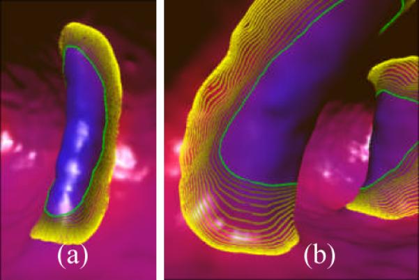
Examples of the evolution processes on two folds. The green thick curves show the IFBs, and the curves from gray yellow to bright yellow indicate the intermediate iso-contours every ten iteration steps, while the brightest yellow curves denote the final segmentation results. (a) The fold as in Figure 3(a). (b) The fold as in Figure 3(b).

III. Evaluation

A. CTC data base

For evaluation, we randomly selected 15 CTC scans, among which 12 are from University of Wisconsin Hospital and Clinics, and the rest from the public WRAMC database [2]. Different CTC techniques, like bowel preparation and imaging protocols, were used to generate these scans, and they have various resolutions as well as image dimensions.

B. Ground-truth establishment

Unlike previous fold detection methods (as in section I), we invited experts to manually draw the fold boundaries. The manually established boundaries served as the ground truths for validation. To ease the drawing, we firstly flattened the colon surface into a 2D plane [40]. Experts drawn the fold boundaries in the plane, and results were reversed back to 3D as the fold boundaries. A tool was specially designed to implement such procedure. As shown in Figure 9,

• 1)
  The left pane showing 2D flattened colon allows users to

  • draw fold boundaries manually, where the fold areas inside the boundaries are determined automatically;
  • delete dissatisfied fold boundaries;
  • merge two isolated parts of one fold when the fold is cut by the flattening process;
  • save current results automatically in hard drive, and then continue to work out the rest in another session;
  • zoom in/out and move the displayed object, so that experts can check the whole flattened colon;
  • tune the light properties, especially the position, to improve the conspicuity of the boundaries.
• 2)
  The right pane showing 3D colon allows users to

  • zoom in/out, move and rotate the 3D colon surface, so that experts can check every corner of the colon;
  • visualize the fold boundaries, which are reversed from the 2D drawings.
• 3)The two panes communicate in a way that if user hover the mouse on a fold in the 2D plane, its 3D counterpart is highlighted in red, as arrowed in Figure 9. The communication helps user identify the matched pairs.

Figure 9.

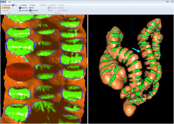
The software interface used to establish the ground truth. The left pane shows the 2D flattened colon surface where the shadow effect is visualized by the normal directions at the vertices in the original 3D colon surface. The right pane shows the 3D colon surface. In both panes, the fold boundaries from experts are in blue color, and the areas inside the boundaries are green color. The arrow-pointed red folds in left and right panes indicate a matched pair in 2D and 3D.

With the tool, the folds of the chosen 15 patient scans were manually plotted by the experts. Anatomically, triple folds circumferentially form a contraction ring on most colon wall, except for the cecum, the lower part (neighboring to the rectum) of the sigmoid colon, and the rectum [41]. However, due to insufficient air inflation and colon bending turns, some folds were greatly expanded and became very shallow and even flat. Therefore, the experts experienced difficulty in locating the accurate boundaries (concave valleys). Fortunately, the number of such folds in a patient scan is usually small and the experts could just ignore them as non-significant folds (as seen in the regions enclosed in the slashed ellipses in Figure 11). Meanwhile, muscles run all over the rectum wall, where the contraction ring of a triple fold could hardly be seen. However, there are turns around there which are likely to be folds. Some of the fold structures near the rectum have been used as spatial reference during clinical image interpretation [42]. Therefore, these structures were drawn as true folds (as seen in Figure 11). As listed in Table 1, there are about 222 folds in average identified by the experts for each patient scan.

Figure 11.

The final segmentation result of one patient scan displayed in a 2D flattened view. From top to bottom, left to right, the images are from the cecum to rectum. The blue thick curves are the expert-drawn fold boundaries, while the green curves are the automatically extracted fold boundaries by the presented algorithm. Arrows indicate the missed folds. There is no false detection observed in the result, while the mismatch between the green and blue curves indicates the local under−/−over segmentation. The regions in the dashed ovals actually contain several folds, whose ground truths are difficult to figure out and so taken as non-significant folds as mentioned in section III.B. However, the dotted rectangle encloses some turns in the sigmoid colon and rectum, which are determined as true folds by both the experts and the segmentation algorithm although they might not be true ones.

Table 1.

The control parameters in the current experiments.

	γ 0	γ 1	γ 2	NM	Δ t
First stage	0.8	0.01	0.1	160	0.4
Second stage	0.003	0.5	10.0

In addition, as mentioned in section II.A, we also used the tool to manually draw curves on folds in the 2D flattened colon. The curves were reversed back to 3D domain, so that we could analyze the curvature characteristics of the colon folds.

C. Control parameters

The parameters γ₀ and γ₁ in equation (7) will weight the a advection terms $\overline{H}$ and $\nabla \overline{H}\cdot \nabla \varphi$. Essentially, the former term would expand ZLSC with a speed adaptive to the intensity of the force image of (5), while the latter one would guide ZLSC to move along the gradient of the force image. Intuitively, the diminished intensity and gradient of the force image would help the convergence of the evolution process. The parameter γ₂ adjusts the last term in equation (7) controlling the smoothness of ZLSC, which prevents the leakage problem [36]. In this study, we employed a two-stage strategy to conduct the LS evolution. In the first stage, such as the first 20 iteration steps, we simply expanded the IFBs by assigning a larger value to γ₀, so that (1) the successive ZLSCs could pass through the whole fold peaks and (2) the whole evolution process could be accelerated. The time step Δt should be limited by the Courant-Friedrichs-Lewy condition so that the numerical convergence of equation (7), i.e., a hyperbolic partial differential equation [43], is ensured. Therefore, in this study, we tried to assign a small value to the time step to ensure a robust performance, while employed a large maximal step to guarantee a complete segmentation. Based on our database, these parameters were determined with the method of trial and error, as listed in Table 1. In the experiments, we fixed all these parameters for all patient scans.

D. Evaluation measures

The performance of the proposed algorithm was measured on a per-fold basis. Given the expert-established ground truth, a fold was assumed to be successfully detected if more than a percentage η of its area has been detected. Therefore, we can estimate the rates of true positive (TP rate, i.e., the detection sensitivity) and false positive (FP rate, which is relative to the specificity). In this study, we set η = 0.5.

To measure the segmentation accuracy, we calculated the segmented-area ratio (SAR):

$$\mathit{SAR}=A_o∕(A_t+A_d-A_o),$$ (10)

where A_t is the expert determined area of the fold (ground truth), A_d is the area of the segmented fold, and A₀ is the area of the overlap of the above two areas. Straightforwardly, a larger SAR suggests a better segmentation result. And SAR=1 indicates that the segmented fold perfectly matches the ground truth without any over- or under-segmentation.

IV. RESULTS

Figure 10 illustrates the LS evolution processes on two folds. As can be seen, the iso-contours become denser as approaching to the brightest yellow curves, suggesting that the evolution processes have converged at the fold boundaries.

Figure 11 in last page shows some final segmentation results as compared to the expert-drawn ground truths where the display is on the flattened 2D view. It is noted that in the images, some folds are cut into two parts by the flattening process, where the cutting lines are still displayed as boundaries for the simplicity of processing. As observed, most of the expert-drawn folds are successfully detected, while a few small shallow folds are missed (false negative, FN). According to the established ground truth, there is no non-fold structures detected. The mismatch between the fold boundaries of expert-drawn and automatically-segmented suggests the local under-/over-segmentation. The merits mentioned in section III.D were used to quantitatively measure the performance of the presented segmentation algorithm.

Table 2 lists the quantitative results from the 15 patient scans. Under the condition that a fold would be detected if more than 50% of its area has been segmented, then about 92.7% of all the expert-drawn folds have been detected with approximately 16.2 missed. The missed ones were mostly shallow and flat shaped structures, as shown by the arrows in Figure 11. The FP detections were very few, i.e., about 0.667 for each scan. For all the detected folds, the segmented area ratio (SAR as defined in section III.D) is about 86.2%, indicating that the automatically segmented fold boundaries have matched fairly well with those of the expert-drawn counterparts.

Table 2.

Quantitative results from the 15 patient scans.

Scan ID	#Ground truth	Sensitivity	#FNs	#FPs	SAR
1	196	0.908	18	1	0.813
2	252	0.940	15	0	0.868
3	229	0.882	27	1	0.869
4	209	0.914	18	0	0.845
5	212	0.910	19	0	0.805
6	264	0.936	17	1	0.836
7	225	0.898	23	0	0.852
8	218	0.968	7	1	0.906
9	217	0.954	10	2	0.870
10	234	0.889	26	1	0.847
11	231	0.970	7	0	0.917
12	217	0.926	16	2	0.857
13	219	0.927	16	1	0.867
14	207	0.942	12	0	0.876
15	211	0.943	12	0	0.899
Average	222.7±17.5	0.927 ± 0.027	16.2±6.085	0.667 ± 0.724	0.862 ± 0.031

Columns 2, 4 and 5 indicate the numbers of the expert-drawn folds, false negatives, and false positives on each scan, while columns 3 and 6 are measures by the merits of section III.D. The last row denotes the averages by scan and standard deviations of columns 2 to 6.

Figure 12 shows the result with the 3D endoluminal display. The presented algorithm segmented the boundaries of most folds from rectum to cecum. The circumferentially neighboring folds, i.e., the horizontally-neighboring folds in Figure 11, are clearly differentiated.

Figure 12.

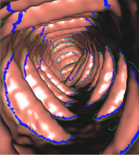
3D endoluminal display of the final segmentation. The blue thick curves show the expert-drawn fold boundaries, while the green curves denote the computer-segmented fold boundaries.

V. Discussion and Conclusion

In this study, we presented an automated algorithm to segment the fold surface in human the colon. The innovation of this work lies in: (1) the whole fold boundary is clearly modeled based on the differential geometry analysis; (2) the model fits naturally into a LS framework for fold segmentation; (3) a software or user-interface tool is designed to assist the experts to manually figure out the fold boundaries as ground truth; and (4) based on the established ground truth, a solid quantitative evaluation has been made.

Compared to the expert-drawn folds on 15 patient scans, the experimental results have shown that 92.7% of all folds are successfully detected with very few false positives. However, we notice that there are previous works focusing on fold detection (as in Section I). Comparing the detection performance with previous works could make the study more complete. Unfortunately, the inaccessibility to others' code makes this task difficult and we leave it as a future work.

The high SAR value of 86.2% shows a good match to the expert-drawn ground truth among the detected folds. Such good performance roots from the model of characterizing the folds and the embedment of the model into the LS framework. The results suggest that the output of the segmentation algorithm can be directly fed into our next work, like fold-segmentation-based TC extraction, with the goal of colon decomposition as mentioned in Section I based on the fold boundaries, fold peaks and TC.

Post-procedures, like TC extraction and supine-prone registration, have already attracted much attention [11–19]. However, as mentioned in Section I, most works are just based on fold detection, which means that only the fold peaks serve as the assistant references. However, our fold segmentation will provide the fold boundaries, which are closed, complete and isolated without overlaps in the circumferential direction. For TC extraction, the isolation property will help locating the TC, since TC are in-between folds. For supine-prone registration, we believe the fold boundaries will provide extra reference information when designing the similarity measures. Parts of our future work will be dedicated to evaluate these points.

The presented segmentation algorithm is solely similar to [22] by sharing the common strategy of utilizing the LS method. However, Chowdhury et al. employed a function of the shape index and curvedness to establish the force term, while we used the mean curvature which is based on the model and characteristic analysis of the fold in sections II.A and II.F.2. The initialization step in the LS framework is extremely important for the evolution process. Chowdhury et al. applied a heat diffusion and fuzzy C-means strategy to extract the initial folds, where the yielded initial folds could cross the fold boundaries and lead to un-desired results. By observing Figure 6(c) in [22], the three folds on one contraction ring were frequently detected as one fold, which may render difficulties for following applications like TC extraction. Such issue can hardly be seen in our results because fold peaks were extracted to serve as the initial folds with a large threshold of the shape index (as described in section II.E). Furthermore, similar to many previous reports, the lack of ground truth has hindered the delivery of quantitative evaluation in [22], and the lacking in quantitative evaluation would limits their work more likely into the category of fold detection, rather than fold segmentation, as mentioned in Section I.

It should be noted that the proposed fold model in Section II.A depends on the mean curvature H, which is essentially related to the concavity of the fold boundaries. It would be beneficial to keep in mind that there exist extreme cases with under/over distended colons. These extreme cases might fail the proposed fold model, and lead to undesired results. Figure 11 shows an over distended colon, where there are number of folds (indicated by arrows and dashed oval) being expanded by the air-pressure and appearing flat and shallow. The arrowed shallow folds in Figure 11 can be captured by human observers. However, the weak concavity at their boundaries fails the fold model and they are missed as false negatives. In addition, the folds in the dashed oval are too flat to be detected by both the human observer and the fold segmentation algorithm. Initially, we do have two under distended colons in our database. However, the under distension leads to collapses. As a result, the segmented colons miss some parts of the colon, and some folds directly touch the haustrals and lose their boundaries in the segmented colon wall. Both results present difficulties for experts to draw the ground truth. Considering the huge efforts for drawing the ground truth, we temporarily report the results with the current database. However, we do understand that there are interesting questions we need to answer. What is the performance with under/over distended colons? To fully exploit the proposed algorithm, do we need to suggest an optimized air pressure during bowel preparation? If yes, what is it? Further study is needed to address these questions.

Polyps may sit on the fold boundaries by chance, as shown in Figure 13. Fortunately, the concave structure between the polyp and the neighboring fold is still consistent with the fold characteristic analysis in section II.A and, therefore, the segmented fold boundary would bend without passing through the polyp. It is noted that the goal of CTC is polyp detection, so such bended fold boundary is clinically acceptable. Polyps may also sit on the fold side between the fold's boundary and peak, which may lead to un-desired segmentation result if the polyp is outside the initial fold boundary. In such case, the fold boundary may hang on the polyp. In our current patient database, we do not find such case. Therefore, further analysis is needed to address this issue with expanded database.

Figure 13.

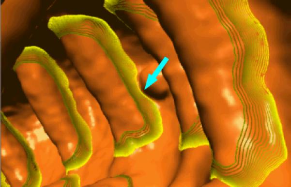
The segmentation result a patient colon at the same location as that of Figure 7(b). The green and yellow curves are as depicted in Figure 10. The arrow indicates the segmented fold boundary around a polyp.

In conclusion, we have presented a fully automatic fold segmentation algorithm. For the first time, expert-drawn ground truth was utilized to conduct a quantitative evaluation. The experimental results are promising upon an experimental database without severe under/over colon distension, implying the potential of benefiting various post-procedures, such as TC extraction, colon decomposition, supine-prone registration, polyp detection, polyp matching, synchronized virtual navigation, etc. As future work, the algorithm shall be tested on more patient studies to show its robustness in various clinical conditions, especially the various degrees of colon distension.

References

- [1].American Cancer Society . Cancer Facts & Figures 2008. American Cancer Society; Atlanta: 2008. [Google Scholar]
- [2].Summers R, Yao J, Pickhardt P, Franaszek M, Bitter I, Brickman D, Krishna V, Choi R. Computed tomographic virtual colonoscopy computer-aided polyp detection in a screening population. Gastroenterology. 2005;129:1832–1844. doi: 10.1053/j.gastro.2005.08.054. [DOI] [PMC free article] [PubMed] [Google Scholar]
- [3].Zhu H, Liang Z, Pickhardt P, Barish M, You J, Fan Y, Lu H, Posniak E, Richards R, Cohen H. Increasing computer-aided detection specificity by projection features for CT colonography. Medical Physics. 2010;37(4):1468–1481. doi: 10.1118/1.3302833. [DOI] [PMC free article] [PubMed] [Google Scholar]
- [4].Pickhardt P, Choi J, Hwang I, Butler J, Puckett M, Hildebrandt H, Wong R, Nugent P, Mysliwiec P, Schindler W. Computed tomographic virtual colonoscopy to screen for colorectal neoplasia in asymptomatic adults. New England Journal of Medicine. 2003;349(23):2191–2200. doi: 10.1056/NEJMoa031618. [DOI] [PubMed] [Google Scholar]
- [5].Taylor S, Iinuma G, Saito Y, Zhang J, Halligan S. CT colonography: computer-aided detection of morphologically flat T1 colonic carcinoma. European Radiology. 2008;18(8):1666–1673. doi: 10.1007/s00330-008-0936-7. [DOI] [PubMed] [Google Scholar]
- [6].de Vries A, Jensch S, Liedenbaum M, Florie J, Nio C, Truyen R, Bipat S, Dekker E, Fockens P, Baak L, Stoker J. Does a computer-aided detection algorithm in a second read paradigm enhance the performance of experienced computed tomography colonography readers in a population of increased risk? European Radiology. 2009;19:941–950. doi: 10.1007/s00330-008-1215-3. [DOI] [PubMed] [Google Scholar]
- [7].Summers R, Johnson C, Pusanik L, et al. Automated Polyp Detection at CTC: Feasibility assessment in a human population. Radiology. 2001;219:51–59. doi: 10.1148/radiology.219.1.r01ap0751. [DOI] [PubMed] [Google Scholar]
- [8].Yoshida H, Nappi J. Three-dimensional computer-aided diagnosis scheme for detection of colonic polyps. IEEE Transactions on Medical Imaging. 2001;20(12):1261–1274. doi: 10.1109/42.974921. [DOI] [PubMed] [Google Scholar]
- [9].Pickhardt P, Taylor A, Gopal D. Surface visualization at 3D endoluminal CT colonography: Degree of coverage and implications for polyp detection. Gastroenterology. 2006;130(6):1582–1587. doi: 10.1053/j.gastro.2006.01.044. [DOI] [PubMed] [Google Scholar]
- [10].Yao J, Summers R. Detection and segmentation of colonic polyps on haustral folds. Proc. Fourth IEEE International Symposium on Biomedical Imaging (ISBI); Metro Washington DC, USA. 2007. pp. 900–903. [Google Scholar]
- [11].Huang A, Roy D, Franaszek M, Summers R. Teniae coli guided navigation and registration for virtual colonoscopy. IEEE Visualization. 2005:279–283. [Google Scholar]
- [12].Huang A, Roy D, Summers R, Franaszek M, Petrick N, Choi J, Pickhardt P. Teniae coli-based circumferential localization system for CT colonography: Feasibility study. Radiology. 2007;243(2):551–560. doi: 10.1148/radiol.2432060353. [DOI] [PubMed] [Google Scholar]
- [13].Lamy J, Summers R. Teniae coli detection from colon surface: Extraction of anatomical markers for virtual colonoscopy. LNCS. 2007;4841:199–207. [Google Scholar]
- [14].Zhu H, Li L, Fan Y, Lin Q, Lu H, Liang Z. Automatic teniae coli detection for computed tomography colonography. Proc. SPIE Medical Imaging 2011. 2011;7963:7963N–1. [Google Scholar]
- [15].Acar B, Napel S, Paik D, Li P, Yee J, Beaulieu C, Jeffrey R. Registration of supine and prone CT colonography data: Method and evaluation. Radiology. 2001;221:332. [Google Scholar]
- [16].Nappi J, Okamura A, Frimmel H, Dachman A, Yoshida H. Region-based supine-prone correspondence for the reduction of false-positive CAD polyp candidates in CT colonography. Academic Radiology. 2005;12:695–707. doi: 10.1016/j.acra.2004.12.026. [DOI] [PubMed] [Google Scholar]
- [17].Wang S, Yao J, Liu J, Petrick N, van Uitert R, Periaswamy S, Summers R. Registration of prone and supine CT colonography scans using correlation optimized warping and canonical correlation analysis. Medical Physics. 2009;36(12):5595–5603. doi: 10.1118/1.3259727. [DOI] [PMC free article] [PubMed] [Google Scholar]
- [18].Fukano E, Oda M, Kitasaka T, Suenaga Y, Takayama T, Takabatake H, Mori M, Natori H, Nawano S, Mori K. Haustral fold registration in CT colonography and its application to registration of virtual stretched view of the colon. Proc. SPIE Medical Imaging 2010. 2010;7624:762420. [Google Scholar]
- [19].Zeng W, Marino J, Gurijala K, Gu X, Kaufman A. Supine and prone colon registration using quasi-conformal mapping. IEEE Transactions on Visualization and Computer Graphics. 2010;16(6):1348–1357. doi: 10.1109/TVCG.2010.200. [DOI] [PMC free article] [PubMed] [Google Scholar]
- [20].Wei Z, Yao J, Wang S, Summers R. Teniae coli extraction in human colon for computed tomographic colonography images. Proc. MICCAI 2010 workshop: Virtual Colonoscopy & Abdominal Imaging; Beijing, China. 2010. pp. 135–140. [Google Scholar]
- [21].Oda M, Kitasaka T, Mori K, Suenaga Y, Takayama T, Takabatake H, Mori M, Natori H, Nawano S. Haustral fold detection method for CT colonography based on difference filter along colon centerline. Proc. SPIE Medical Imaging 2009. 2009;7260:72602M–1. [Google Scholar]
- [22].Chowdhury A, Tan S, Yao J, Summers R. Colonic fold detection from computed tomographic colonography images using diffusion-FCM and level sets. Pattern Recognition Letters. 2010;31(9):876–883. [Google Scholar]
- [23].Zhu H, Li L, Fan Y, Liang Z. Haustral fold segmentation of CT colonography using ridge line detection. Proc. MICCAI 2010 Workshop of Virtual Colonoscopy & Abdominal Imaging; Beijing China. 2010. pp. 33–39. [Google Scholar]
- [24].Ohtake Y, Belyaev A, Seidel H. Ridge-valey lines on meshes via implicit surface fitting. ACM Transaction on Graphics (TOG) 2004;23(3):609–612. [Google Scholar]
- [25].Dorai C, Jain A. COSMOS - A representation scheme for 3D free-form objects. IEEE Transaction on Pattern Analysis and Machine Intelligence. 1997;19:1115–1130. [Google Scholar]
- [26].Liang Z, Wang S. An EM approach to MAP solution of segmenting tissue mixtures: a numerical analysis. IEEE Transactions on Medical Imaging. 2009;28(2):297–310. doi: 10.1109/TMI.2008.2004670. [DOI] [PMC free article] [PubMed] [Google Scholar]
- [27].Wang S, Li L, Cohen H, Mankes S, Chen J, Liang Z. An EM approach to MAP solution of segmenting tissue mixture percentages with application to CT-based virtual colonoscopy. Medical Physics. 2008;35(12):5787–5798. doi: 10.1118/1.3013591. [DOI] [PMC free article] [PubMed] [Google Scholar]
- [28].Lorensen WE, Cline HE. Marching cubes: A high resolution 3D surface construction algorithm. Computer Graphics. 1987;21(4):163–169. [Google Scholar]
- [29].Zhu H, Duan C, Pickhardt P, Wang S, Liang Z. Computer-aided detection of colonic polyps with level set-based adaptive convolution in volumetric mucosa to advance CT colonography toward a screening modality. Cancer Management and Research. 2009;1(1):1–13. doi: 10.2147/cmar.s4546. [DOI] [PMC free article] [PubMed] [Google Scholar]
- [30].Sundaram P, Zomorodian A, Beauleu C, Napel S. Colon polyp detection using smoothed shape operator: preliminary results. Medical Image Analysis. 2008;12:99–119. doi: 10.1016/j.media.2007.08.001. [DOI] [PubMed] [Google Scholar]
- [31].Lipschutz M. Theory and problems of differential geometry. McGraw-Hill; 1969. [Google Scholar]
- [32].Smith L. A tutorial on principal components analysis. 2002 http://www.cs.otago.ac.nz/cosc453/student_tutorials/principal_components.pdf.
- [33].Wan M, Liang Z, Ke Q, Hong L, Bitter I, Kaufman A. Automatic centerline extraction for virtual colonoscopy. IEEE Transactions on Medical Imaging. 2002;21(12):1450–1460. doi: 10.1109/TMI.2002.806409. [DOI] [PubMed] [Google Scholar]
- [34].Maurer C, Qi R, Raghavan V. A linear time algorithm for computing exact Euclidean distance transforms of binary images in arbitrary dimensions. IEEE Transactions on Pattern Analysis and Machine Intelligence. 2003;25(2):265–270. [Google Scholar]
- [35].Sethian J. Level Set Methods and Fast Marching Methods: evolving interfaces in computational geometry, fluid mechanics, computer vision, and materials science. 2nd ed. Cambridge University Press; Cambridge: 1999. [Google Scholar]
- [36].Chan T, Vese L. Active contours without edges. IEEE Transactions on Medical Imaging. 2001;10(2):266–277. doi: 10.1109/83.902291. [DOI] [PubMed] [Google Scholar]
- [37].Duan C, Liang Z, Bao S, Zhu H, Wang S, Zhang G, Chen J, Lu H. A coupled level set framework for bladder wall segmentation with application to MR cystography. IEEE Transactions on Medical Imaging. 2010;29(3):903–915. doi: 10.1109/TMI.2009.2039756. [DOI] [PMC free article] [PubMed] [Google Scholar]
- [38].Barth T, Sethian J. Numerical schemes for the Hamilton-Jacobi and level set equations on triangulated domains. Journal of Computational Physics. 1998;145:1–40. [Google Scholar]
- [39].Mitchell JSB, Mount DM, Papadimitriou CH. The discrete geodesic problem. SIAM Journal on Computing. 1987;16(4):647–668. [Google Scholar]
- [40].Hong W, Gu X, Qiu F, Jin M, Kaufman A. Conformal virtual colon flattening. ACM Symposium on Solid and Physical Modeling. 2006:85–94. [Google Scholar]
- [41].Williams I. Diverticular disease of the colon without diverticula. Radiology. 1967;89(3):401–412. doi: 10.1148/89.3.401. [DOI] [PubMed] [Google Scholar]
- [42].Frimmel H. RSNA 2003. Vol. 474. Chicago: 2003. Reduction of false positives based on supine-prone correspondence for CAD of CT colonography. [DOI] [PubMed] [Google Scholar]
- [43].Courant R, Friedrichs K, Lewy H. On the partial difference equations of mathematical physics. IBM Journal. 1967:215–234. [Google Scholar]