

Abstract
Many brain morphometry studies have been performed in order to characterize the brain atrophy pattern of Alzheimer’s disease (AD). The earliest studies focused on the volume of particular brain structures, such as hippocampus and entorhinal cortex. Even though volumetry is a powerful, robust and intuitive technique that has yielded a wealth of findings, more complex shape descriptors have been used to perform statistical shape analysis of particular brain structures. However, in shape analysis studies of brain structures the information of the relative pose between neighbor structures is typically disregarded. This work presents a framework to analyse pose information including the following approaches: similarity transformations with either pseudo-Riemannian or left-invariant Riemannian metric, and centered transformations with a bi-invariant Riemannian metric. As an illustration, an analysis of covariance (ANCOVA) and a discrimination analysis were performed on Alzheimer’s Disease Neuroimaging Initiative (ADNI) data.
Keywords: Alzheimer’s disease, Pose information, Similarity transformations, Riemannian distance
Introduction
Alzheimer’s disease (AD) is the most common form of dementia. The clinical sign is a progressive cognitive decline initially shown as memory loss, and spreading later to all other cognitive faculties. Mild cognitive impairment (MCI) is a relatively recent concept introduced to recognize the intermediate cognitive state where patients are neither cognitively intact nor demented (Petersen et al., 2001).
The Alzheimer’s Disease Neuroimaging Initiative (ADNI) (Mueller et al., 2005a,b) is a large multi-site longitudinal structural MRI and PET study of about 800 adults, ages 55 to 90, including 200 elderly controls, 400 subjects with mild cognitive impairment, and 200 patients with AD. The ADNI was launched in 2003 by the National Institute on Aging, the National Institute of Biomedical Imaging and Bioengineering, the Food and Drug Administration, private pharmaceutical companies and non-profit organizations, as a $60 million, 5-year public–private partnership. The primary goal of ADNI has been to test whether serial MRI, PET, other biological markers, and clinical and neuropsychological assessment can be combined to measure the progression of MCI and early AD. Determination of sensitive and specific markers of very early AD progression is intended to aid researchers and clinicians to develop new treatments and monitor their effectiveness, as well as lessen the time and cost of clinical trials.
Nowadays several techniques for analysis of brain anatomy are available. The oldest approach is the volumetry technique, which measures the volume of specific brain structures. It relies on the delineation of the regions of interest (ROI). Volumetry is a powerful, robust and intuitive technique that has yielded a wealth of findings. The volume and volume change of particular brain structures such as entorhinal cortex, hippocampus, parahippocampal gyrus, and amygdala (Laakso et al., 1995; Krasuski et al., 1998; Jack et al., 1999; Du et al., 2001, 2003; Pennanen et al., 2004), have been long used as a neuroimaging marker of dementia in both cross-sectional and longitudinal studies.
More specific and subtle shape information of particular regions or structures, such as the hippocampus, has been analyzed by means of statistical shape analysis. In shape analysis theory, shape is often defined as all the geometrical information of an object which is invariant to pose, usually defined as the information about location, orientation and very often size of the object. Therefore, pose and shape provide complementary information about the object of interest. Different shape features have been used so far, such as landmark coordinates (Csernansky et al., 2000, 2004), thickness or radial atrophy maps (Thompson et al., 2007; Querbes et al., 2009), and medial representations (Styner et al., 2003). In all these shape analysis studies of a single structure, the pose information is rejected during an alignment stage because pose mainly depends on irrelevant external factors (e.g. patient’s location and orientation within the scanner).
However, the information of relative pose among different structures belonging to a complex multi-structure system may be useful for diagnosis, prognosis and monitoring. In Rao et al. (2008) the correlation of the anatomical information of the subcortical nuclei was analyzed using point distribution models (PDM) after a global alignment, which can be considered as a joint pose and shape descriptor. A methodology to build statistical pose models was introduced in Bossa and Olmos (2006) where the application was on subcortical nuclei from the normal subjects. Statistical analysis of pose and shape was performed in Bossa and Olmos (2007). The pose and shape of the subcortical nuclei were also analyzed in a longitudinal pediatric study on autism (Styner et al., 2006), with a recent discrimination analysis (Gorczowski et al., 2010).
The aim of this work is twofold. First to revisit a methodology for the statistical analysis of the relative pose information between objects belonging to a multi-object set. A more general presentation is given, including a comparison of the geodesics corresponding to the following approaches: pseudo-Riemannian metrics, left-invariant Riemannian metric on the group of similarity transformations, Sim(3), to our knowledge not done before, and a bi-invariant metric on the group of centered transformations, . The second aim is to assess the usefulness of the pose information of the subcortical nuclei in Alzheimer’s disease. In particular, an analysis of covariance (ANCOVA) of the diagnostic label and an individual classification study between normal subjects and patients were performed using pose parameters as features.
Materials and methods
Subjects
A subset of 554 elderly subjects from ADNI study (Mueller et al., 2005a) was used in this work. All subjects underwent clinical/cognitive assessment, as well as studies of certain AD biomarkers, including apolipoprotein E (ApoE) genotype, at the time of the scan acquisition. There are three common human ApoE isoforms (E2, E3 and E4). Each copy of the ApoE4 allele increases the risk of developing AD, while ApoE2 may have a protective effect (Farrer et al., 1997; Graff-Radford et al., 2002). An integer number, APOEf, was used to quantify the risk of developing AD. The value from 1 to 5 means the following combinations: E2–E2, E2–E3, E2–E4 or E3–E3, E3–E4, and E4–E4, respectively.
As part of each subject’s cognitive evaluation, the Mini-Mental State Examination (MMSE) was performed to provide a global measure of mental status based on the evaluation of five cognitive domains: orientation, attention, calculation, registration, language and recall (Cockrell and Folstein, 1988). The maximum score is 30 corresponding to a normal cognitive status, and scores of 24 or lower are usually consistent with dementia. The Clinical Dementia Rating (CDR) was also assessed as a measure of dementia severity by evaluating six domains: memory, orientation, judgment and problem solving, home and hobbies, personal care and community affairs (Morris, 1993). The ‘sum-of-boxes’ CDR score (CDRSB) is a summary of the different domains with a larger dynamic range (0–18) compared to the global CDR. Higher scores of CDRSB correspond to more severe dementia. The diagnosis of AD was made according to the NINCDS–ADRDA criteria for probable AD (McKhann et al., 1984). More details about the criteria for patient selection and exclusion can be found in the ADNI protocol (Mueller et al., 2005a,b).
The distribution of subjects regarding the patient group was: 207 normal subjects (NOR), 176 AD patients, and 171 subjects with MCI. MCI subjects were divided into two categories: MCI stable (MCIs, N = 89), formed by the subjects who remained with an MCI diagnosis during a 3-year follow-up; MCI converter (MCIc, N = 82), considering patients who converted to AD during the 3-year follow-up. These patient groups will be used to define several disease stages where the performance of the candidate biomarkers will be assessed. It should be noted that clinical evidence of dementia was only available for patients at the AD group, and for patients belonging to the MCIc after the 3-year follow-up. The percentage of MCIs patients that will convert to AD in longer follow-up intervals is unknown. In spite of this limitation, in this work we will use the NOR–MCIs comparison in order to characterize a ‘potential early stage of the disease’, NOR–MCIc as an intermediate stage and NOR–AD as the latest stage of the disease. Table 1 provides a summary of demographic and cognitive scores.
Table 1.
Demographic data and cognitive scores of selected subjects. Age, MMSE and CDRSB format: average (standard deviation, [min, max]).
| Group | Gender |
Age | APOEf |
Baseline |
Baseline |
|---|---|---|---|---|---|
| (M/F) | Distribution | MMSE | CDRSB | ||
| NOR | 101/106 | 76 (5,[62,90]) | (2, 29, 125, 46, 5) | 29 (1,[26,30]) | 0.0 (0.1,[0,0.5]) |
| MCIs | 66/23 | 75 (7,[55,88]) | (0, 4, 50, 31, 4) | 28 (2,[24,30]) | 1.3 (0.6,[0.5,3]) |
| MCIc | 55/27 | 75 (7,[55,88]) | (0, 1, 24, 41, 16) | 27 (2,[24,30]) | 1.9 (1.0,[0.5,5]) |
| AD | 89/87 | 75 (8,[55,91]) | (0, 5, 57, 80, 34) | 23 (2,[20,27]) | 4.3 (1.6,[1,9]) |
MRI acquisition and image correction
High-resolution structural brain MRI scans were acquired at multiple ADNI sites with 1.5 T MRI scanners using the standard MRI protocol developed for ADNI (Jack et al., 2008). For each subject, a T1– 3D MRI scan was collected using a sagittal 3D magnetization-prepared rapid acquisition with gradient echo (MP-RAGE) sequence with voxel size 0.94 mm×0.94 mm×1.2 mm. Additional image preprocessing included geometric distortion correction, bias field correction and geometrical scaling. The images were calibrated with phantom-based geometric corrections to ensure consistency among scans acquired at different sites. The pre-processed images were downloaded from the ADNI website.1
Shape characterization and alignment
Baseline T1 MRI images were analyzed with the FIRST tool, from FSL package (Smith et al., 2004), for automatic segmentation of the following subcortical structures: caudate nucleus, accumbens nucleus, putamen, pallidum, hippocampus, amygdala and thalamus. FIRST is a model-based segmentation/registration tool that uses shape/appearance models. Subcortical structures are parameterized as surface meshes and modeled as a PDM, where point correspondence is assumed. The point distribution was approximately uniform on the surfaces. The number of points (above 600 points) was large considering the object size and its spatial frequency.
Pose parameters are obtained from an alignment procedure. Point correspondence between different subjects for each structure was required because Procrustes alignment was used in this work. Procrustes alignment is a typical method of choice when the shape is characterized as a labeled point set (Dryden and Mardia, 1998). If other shape descriptors are used a different alignment strategy may be better suited. It is worthy to note that the pose parameters will depend on the selected alignment strategy and shape description, including the number and distribution of points in the case of a PDM.
Pose characterization
Two geometric objects A and B have the same shape if there is a geometric transformation T, such that T(A)=B. In this work, T includes translation, rotation and uniform scaling, and is denoted as similarity transformation. More precisely, a point is transformed as
| (1) |
where is a scaling factor, R ∈ SO(3) is a rotation matrix, i.e. R is a 3×3 real matrix such that RRT=RTR=I3 and det(R)=1, and is a 3D vector. Note that the similarity transformations have 7 degrees of freedom. The pose of an object is described by the transformation which relates the local coordinate system of the object (or body-fixed frame) with the global coordinate system (reference frame).
Similarity
The set of similarity transformations defined in Eq. (1) forms a group, denoted here as Sim(3). Let (s,R,b) be the parameters that define T in Eq. (1), then the group operation T2°T1, which is the composition of transformations, can be written in terms of the parameters as
| (2) |
which is obtained by the consecutive application of the transformations T1 followed by T2.
In homogeneous coordinates a similarity transformation is written as
| (3) |
where 0=(0, 0,0)T is the null vector in . It can be checked that matrix multiplication coincides with the composition of transformations.
Centered transformations
There is an alternative characterization of the pose in which the object is rotated and scaled with respect to a center of rotation, , fixed to the object, and finally the center is translated. A similar description is used for rigid body dynamics in physics, where the center of rotation is the center of mass. Each point x of the object can be described by the pair where . The transformation rule of the pair is given by
| (4) |
The group operation T2 °T1 is given now by
| (5) |
therefore the corresponding group is i.e. the direct product of the following 3 groups: means positive changes in the scale, SO(3) means rotations and means translations of the centroid.
The drawback of this parameterization is given by the fact that the pose parameters depend on the choice of c. On the other hand, the corresponding group is the direct product of smaller groups than Sim(3), making the subsequent analysis easier.
Lie group structure of pose transformations
A Lie group is a group which is also a differentiable manifold. Differentiable manifolds are curved spaces that are locally similar to Euclidean spaces. The tangent space at the identity e of a Lie group G, is a vector space denoted Lie algebra . Let be , then there is a diffeomorphism (i.e. a smooth and invertible mapping) denoted exponential map, , from a neighborhood of the origin of g to a neighborhood of the identity e of G. The exponential map provides all the one-parameter subgroups,2 given by curves of the form exp(vt), . The exponential map and its inverse, the logarithm, , are useful because they provide a representation of the group elements in terms of a vector space, where addition and scalar multiplication (i.e. linear combinations) are well defined. In the case of matrix groups, the exponential and logarithm mappings coincide with the standard matrix exponential and logarithm, respectively, allowing the use of fast computation schemes. Direct computation with elements from a Lie group by means of their logarithm representation was named Log–Euclidean framework (Arsigny et al., 2006b). A limitation of the Log–Euclidean framework is the lack of left- and right-invariance, therefore the results are coordinate dependent.
Both, similarity group (Sim(3)) and centered transformations , are Lie groups.
- The Lie algebra of the group is given by the direct product of the corresponding Lie algebras, (Baker, 2002), where so(3) is the Lie algebra of SO(3) and includes the set of skew–symmetric matrices. Let , then the exponential map is given by
where eA is the matrix exponential of A. Because A is a skew–symmetric 3×3 matrix, it can be written as(6)
then R = eA performs a rotation of angle around an axis given by (θx, θy, θz)/θ. A more detailed analysis of computing statistics on SO(3) is given in (Moakher, 2003).(7) - The Lie algebra of Sim(3), denoted sim(3), consists of matrices of the form
where I3 is the 3×3 identity matrix. The exponential mapping is given by the matrix exponential eV. When l=0 (i.e. there is no scaling change) a subgroup of Sim(3) is obtained, denoted special Euclidean group, SE(3), and a point x transformed by etV, describes a ringlet shaped curve denoted screw motion.(8)
Statistics of pose information
In order to perform statistical analysis on the elements of a Lie group G, a distance d(g, h) between elements g,h∈G must be defined. Lie groups are also Riemannian manifolds, and distances are defined by selecting a Riemannian metric. Distances in Riemannian manifolds are given by the length of the geodesic curve (the shortest path on the manifold) connecting two elements. The Riemannian exponential, Expg :TgG→G, is a local diffeomorphism that maps vectors from the tangent space at g of G, TgG, to elements on the manifold, such that Expg(tv), 0≤t≤1, is a geodesic starting at g, with initial velocity v and whose length is , where ⟨ ·, · ⟩g is a Riemannian metric at g. Its inverse function is the Riemannian logarithm, Logg :G → TgG,
| (9) |
that is related to the Riemannian distance by d(g, h)= ∥Logg(h)∥.
Metrics on Lie groups, and their induced distances, can be divided into left-invariant (d(g1, g2)=d(h°g1, h°g2)), right-invariant (d(g1,g2)= d(g1°h, g1°h)) and bi-invariant. Left-invariance means that the distance between two pose elements do not depend on the choice of the reference frame. On the other hand, right-invariant metrics provide distances that are invariant to the choice of the object body-fixed frame.
When a bi-invariant metric can be selected, geodesics coincide with translated one-parameter subgroups (Sternberg, 1964) and any geodesic can be written as g° exp(tv) for some g∈G and ν∈g. In particular, the geodesic from g1 to g2 is given by
| (10) |
where and 0 ≤t≤ 1. The length of this geodesic is , where ⟨ ·, · ⟩e is the bi-invariant Riemannian metric at the origin. In the case of centered transformations, , each of its building subgroups admit bi-invariant metrics. Therefore admits bi-invariant metrics and the geodesics can be computed as one-parameter subgroups by means of Eq. (10). The distance between two centered transformations T1 and T2 is given by
| (11) |
where nR,ns, nT>0 are the weights corresponding to the rotation, scaling and translation components, respectively.
Unluckily, a bi-invariant metric cannot always be defined. In these cases the left-invariance is often preferred because it is a key requirement in a larger set of applications. This is the case of the similarity group Sim(3), where there is no bi-invariant metric due to the lack of a bi-invariant metric on the simpler group SE(3) as it was shown in Park (1995). A way of constructing left-invariant geodesics on Sim(3) is given in Appendix A.
When there is no bi-invariant Riemannian metric, and bi-invariant geodesics are still required, a bi-invariant pseudo-Riemannian metric can be defined. The drawback of pseudo-Riemannian metrics, is that there are zero-length geodesics connecting different elements in the manifold (i.e. there are pairs of unequal elements whose distance is zero). Geodesics for the bi-invariant pseudo-Riemannian metrics are given by the one-parameter subgroups. The pseudo-Riemannian metrics on the SE(3) group were described in Park (1995); Zefran et al. (1996, 1999) in the context of rigid body kinematics, and in the case of general lineal transformations (pose+shearing) in (Woods, 2003).
Fig. 1 illustrates the trajectory of an object following a geodesic generated by each one of the following metrics:
One-parameter subgroups on Sim(3): they are the most invariant trajectories. However, a Riemannian metric cannot be defined, and either a pseudo-Riemannian metric is used and zero-length geodesics may appear, or a Log–Euclidean framework is used where distances are non-invariant.
Left-invariant geodesics on Sim(3): they depend on weighting factors and on the choice of the object local (body-fixed) frame. It is important to note that the evolution of the scaling factor s is non-monotonic along this trajectory, even in the case of a geodesic connecting two pose elements where the object size is preserved. In this case, the scale component of the initial velocity would be non-zero, and statistics are computed on the initial velocity. This is an undesirable effect when analyzing the pose subcortical brain structures, because it can be erroneously concluded that there is a scale difference between two object poses while they actually have the same size.
Bi-invariant geodesics on centered transformations: they do not depend on either reference, or body-fixed frames. Additionally, they do not depend on the weighting factors (nR,ns and nT). But they depend on a center of rotation c that is defined on the body-fixed frame.
Fig. 1.
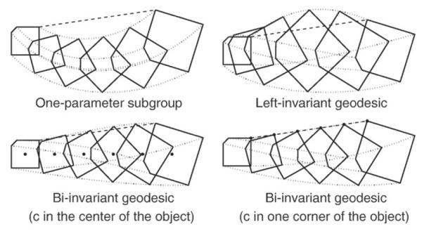
Example of a square object following a trajectory given by: Sim(3) one-parame ter subgroup (top-left); Sim(3) left-invariant geodesic (top-right); centered transformations with center c in the center of the object (bottom-left); and centered transformations with center c at the top-right corner (bottom-right). In bottom panels, the center c is indicated with a dot. A straight dashed-line connecting the top-right corner of the object from initial to end pose is shown for comparison purposes.
In our opinion, the most natural pose characterization for the application of subcortical nuclei is given by the bi-invariant geodesics on centered transformations when the center c is appropriately chosen. For the rest of the paper, only the characterization with centered transformations was used, with center c defined as the center of mass of the object.
Bi-invariant mean
Given a set of objects, it is very common to define a center or representative object of the population under study, e.g. the mean is a typical choice. Let gi be a set of elements belonging to a Riemannian manifold M, and d(·, ·) a distance function, the Karcher mean m is defined as (Karcher, 1977)
| (12) |
When M is a Lie group that admits bi-invariant metrics, the Karcher mean is denoted as bi-invariant mean (Arsigny et al., 2006a), and it can be computed iteratively as follows (Pennec et al., 2006):
| (13) |
Further statistical analysis is performed on vectors vi=log(m−1°gi).
Relative pose in multi-object complexes
When dealing with a joint analysis of a set of structures, such as subcortical nuclei within the brain, the global pose is non-informative because it mainly depends on external factors, such as patient’s pose within the scanner. However, the relative pose between objects may be a relevant information, but it was disregarded in many previous morphometry studies focused on a single brain structure (Styner et al., 2004; Ho and Magnotta, 2010; Gerardin et al., 2009; Sabattoli et al., 2008; Thompson et al., 2004).
Global pose accounts for the position and orientation of patients within the scanner, and head size, which are confounding factors. Original MR images were aligned to a reference image by means of a linear transformation (12 degrees of freedom). For each subcortical structure, residual pose is obtained by means of Procrustes alignment of the set of surface points. Regarding the scale parameter, a very common approach is to normalize the point coordinates by the squaredsum of their values, yielding a representation on the unit 3n-sphere, where n is the number of points. Note that this scale factor depends on the number and distribution of the points on the surface. An alternative scale normalization is used in this work which is more directly related to the volume of the object: landmark coordinates are divided by the cube root of the volume yielding a shape description with unit-volume.
The reference object for each subcortical structure k was defined as the Procrustes mean shape Mk across subjects (Dryden and Mardia, 1998). The pose Ti,k of each structure and each subject i was obtained by Procrustes alignment with the corresponding mean shape Mk. The mean pose was computed using Eq. (13). Fig. 2 illustrates the mean shape at the corresponding mean pose of the selected structures. Subsequent statistical analysis was performed on , i.e. after mean pose subtraction, because they belong to an Euclidean space and their norms are equal to the distances from the group elements to the overall mean pose.
Fig. 2.
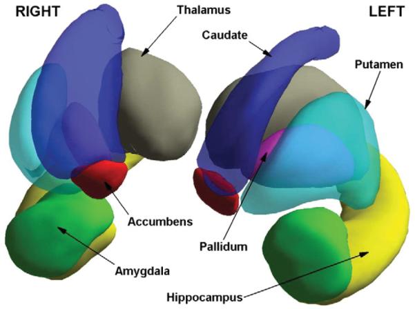
Illustration of the mean pose (and mean shape) of the subcortical nuclei analyzed.
Statistical analysis
For the statistical analysis, the pose parameters were divided in three natural categories: rotation, translation and scale. Univariate (for scale) or multivariate (for rotation and translation) analyses of covariance (M)ANCOVA were performed in order to identify those pose parameters showing statistically significant differences between patient groups. The parameters of each pose category were considered as dependent variables and the group label was the only independent variable. Gender, age and handedness were considered as confounding variables. (M)ANCOVA model assumptions about homoscedasticity and Gaussianity were checked with Box’s M and Lilliefors tests, respectively.
Correction for multiple comparisons was performed using a Bonferroni criterion approach. The total number of models was the product of 3 pose categories and 14 subcortical structures. Accordingly, the p-value threshold was set to 0.05/(3×14) = 1.2×10⁻³.
Note that the MANCOVA was performed on a single tangent space at the overall mean pose, which is valid when pose variations are small. A more rigorous approach would be to compute distances on the tangent space at the mean of each group, as it was recently done in Kendall’s shape space (Huckemann et al., 2010).
Classification analysis
The assessment of the discrimination ability of the pose features was performed using two techniques: standard Linear Discriminant Analysis (LDA), and Distance-Weighted Discrimination (DWD) (Marron et al., 2007).
DWD is a method similar to Support Vector Machines (SVMs), but all sample points are used in the calculation of the discriminating axis. Each point’s contribution to the calculation is weighted inverse proportionally to the distance from that point to the opposite population. The DWD achieves a high robustness for high-dimensional feature spaces with low sample sizes (HDLSS). The software for DWD classification algorithm was downloaded from the author’s web page with suggested parameters. Although pose parameter analysis does not suffer from HDLSS problem, the total number of pose parameters in this study was 98 (14 subcortical structures with 7 pose parameters for each structure), which is pretty high compared to the number of subjects (188 in the smallest group). It is expected that the DWD approach will provide a higher generalization and robustness than LDA.
Four sets of input parameters for the classifiers were defined:
The 14 scale factors, because many previous neuroimaging studies use only volume information for classification: 14 dimensions.
The whole set of pose parameters: 7×14 = 98 dimensions.
The scale parameters together with gender, age and APOE genotype information: 14 + 3 = 17 dimensions.
The whole set of pose parameters together with gender, age and APOE genotype information: 98 + 3 = 101 dimensions.
Classification performance was assessed by means of cross-validation on independent training and testing datasets. The training set (65% of the subjects, 135 NOR, 114 AD, 58 MCIs and 53 MCIc) and testing set (35% of the subjects, 72 NOR, 62 AD, 31 MCSs and 29 MCIc) were randomly selected. This random subsampling was repeated 100 times and the average classification accuracy was measured.
Results
MANCOVA
The first experiment was to assess statistically significant differences in the pose parameters of the subcortical nuclei from the different patient groups. Table 2 collects the p-values corresponding to the (M)ANCOVA analysis when comparing groups at different stages of the neurodegenerative process: NOR vs MCIs, NOR vs MICc and NOR vs AD. The differences in the MCIs–MCIc comparison were not statistically significant after correction for multiple comparisons. For brevity reasons, only the results for the explanatory variables are given, although the confounding variables gender and age were also statistically significant in many subcortical structures while handedness was not significant for any structure. To facilitate a comparison with volumetry studies, the average of the normalized volume difference, , is given in Table 3.
Table 2.
Statistical significance (p-value) of the (M)ANCOVA of the subcortical nuclei pose parameters vs Group variable. Results are given for each pose category and each structure fromboth hemispheres. Shaded cells denote significant values after correction formultiple comparisons using Bonferroni criterion (p<0.05/42=1.2E–3).
| Rot L | Rot R | Trans L | Trans R | Scale L | Scale R | ||
|---|---|---|---|---|---|---|---|
|
| |||||||
| NOR - AD | Amyg. | 4.0E-15 | 1.0E-17 | 9.9E-08 | 3.1E-05 | 4.6E-05 | 6.8E-08 |
| Hipp. | 3.1E-15 | 3.5E-05 | 5.2E-07 | 2.7E-05 | 2.6E-25 | 4.7E-26 | |
| Caud. | 2.3E-07 | 1.9E-05 | 6.9E-10 | 1.5E-08 | 3.7E-01 | 2.3E-01 | |
| Pall. | 5.3E-02 | 6.7E-02 | 4.8E-08 | 1.7E-05 | 1.8E-02 | 1.1E-03 | |
| Thal. | 1.2E-02 | 5.3E-02 | 1.9E-06 | 1.1E-03 | 9.4E-08 | 7.2E-09 | |
| Accu. | 1.7E-02 | 2.3E-02 | 1.3E-06 | 7.3E-06 | 3.7E-05 | 1.3E-08 | |
| Puta. | 2.2E-03 | 4.8E-02 | 1.4E-07 | 3.5E-06 | 7.3E-05 | 2.9E-04 | |
|
| |||||||
| NOR - MCIc | Amyg. | 3.0E-05 | 4.5E-04 | 6.9E-05 | 1.1E-02 | 6.5E-03 | 1.4E-03 |
| Hipp. | 4.7E-02 | 1.1E-01 | 9.9E-04 | 8.8E-04 | 8.2E-010 | 2.5E-09 | |
| Caud. | 3.3E-01 | 4.5E-01 | 6.5E-05 | 3.9E-03 | 9.2E-01 | 7.1E-01 | |
| Pall. | 6.7E-01 | 7.4E-01 | 9.0E-05 | 2.4E-02 | 3.4E-01 | 5.9E-02 | |
| Thal. | 6.7E-01 | 5.3E-01 | 7.4E-04 | 6.3E-03 | 5.8E-04 | 9.7E-04 | |
| Accu. | 6.8E-01 | 4.6E-01 | 1.3E-04 | 3.0E-02 | 8.1E-02 | 6.9E-04 | |
| Puta. | 7.7E-01 | 3.2E-01 | 2.0E-04 | 2.8E-02 | 6.0E-03 | 6.3E-02 | |
|
| |||||||
| NOR - MCIs | Amyg. | 1.3E-01 | 4.0E-01 | 8.3E-02 | 5.5E-01 | 2.0E-02 | 3.2E-02 |
| Hipp. | 4.3E-02 | 4.1E-01 | 4.3E-01 | 3.5E-01 | 2.1E-04 | 3.2E-04 | |
| Caud. | 2.9E-02 | 2.7E-01 | 4.6E-02 | 1.2E-01 | 9.0E-01 | 2.8E-01 | |
| Pall. | 5.4E-01 | 5.7E-01 | 1.8E-01 | 3.3E-01 | 6.8E-02 | 4.4E-2 | |
| Thal. | 8.5E-01 | 5.4E-01 | 1.4E-01 | 4.7E-01 | 1.1E-03 | 9.0E-04 | |
| Accu. | 8.7E-01 | 5.6E-01 | 5.2E-01 | 3.7E-01 | 7.5E-01 | 1.4E-01 | |
| Puta. | 1.1E-01 | 6.3E-01 | 9.6E-02 | 3.2E-01 | 1.6E-01 | 1.2E-01 | |
Table 3.
Difference of normalized volume between patient groups. Shaded cells denote statistically significant values.
| NOR-AD | Amyg. | Hipp. | Caud. | Pall. | Thal. | Accu. | Puta. |
|---|---|---|---|---|---|---|---|
| Left | 7 | 16 | 1 | 3 | 4 | 11 | 5 |
| Right | 11 | 16 | 2 | 3 | 5 | 16 | 4 |
| NOR-MCIc | Amyg. | Hipp. | Caud. | Pall | Thal | Accu | Puta |
| Left | 7 | 12 | 1 | 3 | 5 | 7 | 5 |
| Right | 9 | 12 | 2 | 3 | 4 | 12 | 3 |
| NOR-MCls | Amyg. | Hipp. | Caud. | Pall | Thal | Accu | Puta |
| Left | 7 | 9 | 2 | 5 | 5 | 3 | 3 |
| Right | 7 | 8 | 4 | 4 | 5 | 6 | 3 |
In order to provide a rough illustration of the pose differences between the patient groups, the mean pose of each patient group was applied to the mean shape of each structure after global alignment. Fig. 3 shows the contours of the subcortical structures at their mean pose.
Fig. 3.

Illustration of the mean pose of subcortical nuclei for each patient group.
Classification
Regarding the classification analysis, the average accuracy score of the 100 runs of the cross-validation is shown in Table 4. As expected, the DWD method provided a better generalization than LDA, as can be seen from the difference of the performance between training and testing sets. There is a slight improvement of accuracy when considering the group comparisons in the order of the disease stages MCIs, MCIc and AD. In general, the introduction of a larger amount of information (from only the scale parameters to the whole set of pose parameters together with the demographic information) yields a slightly improved accuracy performance in both, training and testing sets. The inclusion of gender, age and genetic information also increases the accuracy.
Table 4.
Classification accuracy for discrimination between patient groups. Format: average (standard deviation) [min, max]. Shaded cells denote accuracy for pose features.
| Scale parameters | ||||||
|---|---|---|---|---|---|---|
| NOR-AD | NOR-MCIc | NOR-MCls | ||||
| IDA | DWD | LDA | DWD | LDA | DWD | |
| Test | 0.73 (0.03) [0.65,0.80] |
0.73 (0.03) [0.66,0.82] |
0.67 (0.04) [0.57,0.761 |
0.72 (0.03) [0.64,0.79] |
0.59 (0.04) [0.50,0.681] |
0.70 (0.03) [0.62,0.75] |
| Train | 0.76 (0.02) [0.70,0.80] |
0.77 (0.02) [0.71,0.82) |
0.73 (0.03) [0.66,0.79] |
0.78 (0.02) [0.74,0.84) |
0.65 (0.03) [0.57,0.73] |
0.75 (0.02) [0.71,0.79] |
| Pose parameters | ||||||
| Test | 0.75 (0.04) [0.66,0.87] |
0.78 (0.03) [0.72,0,84] |
0.65 (0.05) [0.54,0.77] |
0.76 (0.02) [0.68,0.82] |
0.57 (0.04) [0.47,0.65] |
0.71 (0.02) [0.66,0.76] |
| Train | 0.93 (0.02) [0.89,0.96] |
0.82 (0.01) [0.80,0.86] |
0.94 (0.02) [0.89,0.97] |
0.81 (0.01) [0.79,0.87] |
0.89 (0.02) [0.84,0.95] |
0.78 (0.01) [0.74,0.81] |
| Scale parameters + age, gender and APOE | ||||||
| Test | 0.77 (0.03) [0.70,0.84] |
0.78 (0.03) [0.71,0.85] |
0.75 (0.04) [0.64,0.82] |
0.78 (0.03) [0.72,0.84] |
0.61 (0.04) [0.51,0.70] |
0.71 (0.03) [0.64,0.77] |
| Train | 0.81 (0.02) [0.76,0.86] |
0.81 (0.02) [0.77,0.86] |
0.79 (0.02) [0.75,0.84] |
0.82 (0.02) [0.79,0.86] |
0.69 (0.02) [0.64,0.77] |
0.76 (0.02) [0.72,0.79] |
| Pose parameters + age, gender and APOE | ||||||
| Test | 0.78 (0.04) [0.69,0.87] |
0.80 (0.03) [0.72,0.88] |
0.71 (0.04) [0.60,0.82] |
0.77 (0.02) [0.70,0.83] |
0.58 (0.05) [0.46,0.67] |
0.72 (0.02) [0.67,0.76] |
| Train | 0.95 (0.01) [0.91,0.98] |
0.85 (0.01) [0.82,0.89] |
0.97 (0.01) [0.93,0.99] |
0.82 (0.01) [0.79,0.86] |
0.90 (0.02) [0.84,0.95] |
0.78 (0.02) [0.74,0.82] |
Discussion
Volume can be considered as a simple, coarse and intuitive anatomical descriptor, which is independent of the patient position within the scanner. Many previous ROI-based volumetry studies focused on structures such as entorhinal cortex, hippocampus, and amygdala, which are known to present the largest atrophy at the earliest stages of the neurodegenerative process (Laakso et al., 1996; Apostolova and Thompson, 2008). However, it is known that neurodegeneration spreads over many other regions, in particular over the structures of the limbic system, such as thalami, which are reported less frequently. The statistical techniques to assess significant volume differences are simple univariate hypothesis tests, and correction for multiple comparisons is not an issue. However, volume is an unspecific anatomical descriptor. Recent works show that the shape of a brain structure can be more useful than the volume for population studies (Styner et al., 2004; Csernansky et al., 2000).
More complex shape descriptors typically involve vectors of large dimensionality. For example, shape analysis of a single structure, such as the hippocampus using coordinates of point sets on the surface as shape descriptor, requires thousands of parameters. Statistical analysis on such high dimensional feature space with relatively small sample size (a few hundreds in the best cases) is problematic.
Relative pose information can be regarded as an interesting trade-off for the following reasons. First, the dimensionality required in pose characterization is not very high, just 7 parameters for each structure. Accordingly, the multiple comparison corrections will not be very severe. Second, the pose information3 can be considered as a generalization of volume measurements, because in addition to volume, it provides information about the location and orientation of each object. Third, the pose information is complementary to shape, because the relative pose between structures is typically disregarded in the alignment stage performed in single-structure shape studies.
In this paper a methodology for analysis of the relative pose information from a set of brain structures has been presented. A general framework allowed us to compare several approaches to perform statistical analysis: pseudo-Riemannian metrics, that were proposed in Woods (2003) in the context of linear transformations and in Park (1995); Zefran et al. (1996, 1999) for SE(3) group; Log– Euclidean framework (Arsigny et al., 2006b); left-invariant Rieman-nian metrics on the similarity group, which is, to our knowledge, a novel contribution; and bi-invariant metrics on the group of centered transformations. The first approach can be related to our previous work (Bossa and Olmos, 2006), while the latter approach to Styner et al. (2006); Gorczowski et al. (2010). The comparison of the geodesics induced us to select the bi-invariant centered transformation approach for the following reasons: it avoids the undesirable effect of the non-monotonic trajectories of the scale parameter (see Fig. 1 and discussion below). Moreover, this approach allows a more clear interpretation of the results because the contribution of each natural category, either rotation or translation or scale, are independent. It should be also noted that, to our knowledge, this is the first work where the pose information provides positive results with clinical data, because the pose was useless in a longitudinal study of autism (Styner et al., 2006; Gorczowski et al., 2010) and only normal subjects were considered in our previous work (Bossa and Olmos, 2006).
The application of the methodology was performed in order to illustrate the usefulness of the pose information compared to the volume information in a particular case. To our knowledge, this is the first study considering the whole set of pose parameters of the subcortical nuclei as a potential MRI marker of AD. Although the focus of the paper was devoted to the methodological aspects rather than extracting of clinical useful knowledge from the analyzed data, some interesting results were obtained which deserve discussion.
Regarding the group analysis, it can be seen from Table 2 that the pattern of significant pose differences was different at each group comparison. At the earliest stage of the disease, represented here by the NOR–MCIs comparison, statistical differences were found only for the scale parameter of bilateral hippocampi and thalami. When comparing NOR–MCIc groups, in addition to the previous differences, an important asymmetry was found in the left hemisphere because all subcortical nuclei showed statistically significant translations. It is interesting to note that this left-hemisphere asymmetry was also recently reported in Cherbuin et al. (2010). At the latest stage, when comparing NOR–AD patients, a larger number of subcortical structures showed significant differences in the scale parameter, but also interestingly, translations and rotations were significant in both hemispheres. These pose differences were nicely illustrated in Fig. 3, showing that while some subcortical structures show pose differences along the complete time-course of the disease, such as the hippocampus with an atrophic behavior or caudate nuclei with translations, other structures only experience pose differences at specific stages. Even though pose differences in the MCIs–MCIc comparison were not statistically significant after the correction for multiple comparisons in this dataset, noticeable pose differences can be observed in several subcortical structures in Fig. 3, in some cases almost as large as the ones in the NOR–AD comparison.
On the other hand, Table 3 confirms that the volume of all subcortical structures were smaller in the pathological than in the NOR group, confirming that neurodegeneration is linked to atrophy of subcortical structures. The magnitude of the atrophy increases along the neurodegenerative process, especially of the hippocampi, with cross-sectional atrophy values ranging from 8 to 16%, which are in agreement with the atrophy values reported in the literature (Apostolova and Thompson, 2008). In contrast, caudate nuclei did not show significant volume differences at any disease stage, while presenting significant translation in the left hemisphere for the NOR– MCIc comparison and translations and rotations in both hemispheres for the NOR–AD comparison.
Brain morphometry techniques with better spatial resolution, such as tensor-based morphometry (Bossa et al., 2010; Hua et al., 2008) have shown significant patterns of local atrophy affecting several cortical and subcortical structures. These anatomical changes may be the origin of the observed significant translation and rotation differences of structures such as the hippocampi, in addition to the volume differences. Similarly, significant differences in the translation of structures such as the caudate nuclei, do not experience significant atrophy.
Regarding the classification analysis, a very recent study (Cuingnet et al., in press) compared 10 different methods using the ADNI database (150 subjects for training and 150 for testing). The methods included the assessment of cortical thickness, voxel-based methods, and hippocampus-based approaches. The highest accuracy score for the NOR–AD classification was achieved by whole-brain methods, up to 0.81 sensitivity and 0.95 specificity. The hippocampus-based strategies obtained a similar sensitivity but a lower specificity (between 0.63 for volume based methods and 0.84 for shape based methods). In the case of NOR–MCIc, the sensitivity was substantially lower. In this work, the average accuracy for the NOR–AD classification was equal to 0.78 for the pose parameters, and 0.80 when gender, age and genotype information are considered. The assessment of accuracy was performed in Cuingnet et al. (in press) and in this work with independent training and testing datasets. While Cuingnet et al. (in press) used only a single random allocation of subjects with 50% for training and testing, 100 random allocations with 65% training were used here.
Several limitations of this study can be mentioned. Firstly, as the segmentation of the subcortical nuclei is the starting point, the segmentation errors will have an important influence in the results. Secondly, the current work only looked across individuals at a single snapshot of the evolving process. A longitudinal analysis of the pose changes would be much more convenient in order to get more accurate information about the time-course of the disease. Future studies will be devoted to assess statistical differences between temporal pose changes between different patient groups. Finally, as the pose information is only a coarse descriptor of the anatomy and complementary to shape, better classification results may be obtained with a method with a joint pose + shape statistical analysis, following our preliminary work (Bossa and Olmos, 2007).
Conclusions
A methodology for the analysis of pose information was proposed in this paper. Its application on the ADNI data obtained interesting results both in a population statistical study as well as in classification between control and patient groups. A different pattern of subcortical nuclei pose changes was found at each patient group comparison, which is in agreement with the evolution of the disease. In particular significant differences of translation and rotation parameters were found for NOR vs MCI-converters comparison. These studies confirm the hypothesis that the pose information provides a more detailed description of the anatomical changes induced during the neurodegeneration process than standard volumetry.
Acknowledgments
This work was partially funded by research grants TEC2009-14587-C03-01 from CICYT, PI100/08 from DGA, and CDTI under the CENIT Programme (AMIT Project, CEN-20101014) and supported by the Spanish Ministry of Science and Innovation, Spain. Data collection and sharing for this project was funded by the Alzheimer’s Disease Neuroimaging Initiative (ADNI; Principal Investigator: Michael Weiner; NIH grant U01 AG024904). ADNI is funded by the National Institute on Aging, the National Institute of Biomedical Imaging and Bioengineering (NIBIB), and through generous contributions from the following: Pfizer Inc., Wyeth Research, Bristol-Myers Squibb, Eli Lilly and Company, GlaxoSmithKline, Merck and Co. Inc., AstraZeneca AB, Novartis Pharmaceuticals Corporation, Alzheimer’s Association, Eisai Global Clinical Development, Elan Corporation plc, Forest Laboratories, and the Institute for the Study of Aging, with participation from the U.S. Food and Drug Administration. Industry partnerships are coordinated through the Foundation for the National Institutes of Health. The grantee organization is the Northern California Institute for Research and Education, and the study is coordinated by the Alzheimer’s Disease Cooperative Study at the University of California, San Diego. ADNI data are disseminated by the Laboratory of NeuroImaging at the University of California, Los Angeles.
Appendix A. Left-invariant geodesics on Sim(3)
In Park (1995), geodesics on SE(3) were obtained from the geodesics on SO(3) and using the following theorem: let M1 and M2 be two Riemannian manifolds, and let π: M1 → M2 be a smooth covering map and a local isometry (i.e. a Riemannian covering map), then π maps geodesics into geodesics (Gallot et al., 1987). The mapping πl (πr) for left- (right) invariant metrics, for the SE(3) case, is given by
| (A.1) |
where M1 ≡ SE(3) with the left-(right-)invariant metric having a block-scalar metric tensor at the identity and with the usual bi-invariant metric.
In the case of Sim(3), geodesics can be obtained using an equivalent approach. Let ST(n) be the group of translation and scaling in , which elements are matrices of the form
| (A.2) |
where , . Then, the mapping πl:Sim(3) →SO(3)×ST(3) given by
| (A.3) |
is a Riemannian covering map when Sim(3) and ST(3) are equipped with block-scalar left-invariant metrics, and SO(3) with a bi-invariant metric. Therefore, geodesics on Sim(3) are the liftings of the geodesics on SO(3)×ST(3).
The geodesics on ST(3) can be obtained from geodesics on ST(1) as follows: ST(1) equipped with a left-invariant metric is equivalent to the Poincaré half-plane model (Stahl, 1993), that consists in the upper half of the complex plane with a metric given by ((dx)2 +(dy)2)/y2. Geodesics in this space are given by vertical lines ending in the real axis x + iyet and half-circles whose origins are on the x-axis. All geodesics can be written as (aeti + b)/(ceti + d), where and ad – bc>0. Let b + is → Ts, b be the isomorphism between a complex number in the Poincaré half-plane model and a matrix on ST(1). The distance between T1 = Ts1, b1 and T2 = Ts1, b2 is given by
| (A.4) |
It can be easily seen that a left-invariant geodesic on ST(n) connecting T1 = Ts1, b1 and T2 = Ts2, b2 is given by , where , and γ(t)= r(t)+ is(t) is the geodesic in the Poincaré half-plane model connecting γ(0) ≡ is1 and γ(1) ≡ r + is2.
Footnotes
A curve γ(t) ∈ G is denoted one-parameter subgroup if it is a 1-dimensional group such that γ(t)°γ(s)= γ(t + s), where .
When the scale normalization is selected accordingly.
References
- Apostolova LG, Thompson PM. Mapping progressive brain structural changes in early Alzheimer’s disease and mild cognitive impairment. Neuropsychologia. 2008;46(6):1597–1612. doi: 10.1016/j.neuropsychologia.2007.10.026. [DOI] [PMC free article] [PubMed] [Google Scholar]
- Arsigny V, Commowick O, Pennec X, Ayache N. A log-Euclidean framework for statistics on diffeomorphisms. In: Larsen R, Nielsen M, Sporring J, editors. Proc. MICCAI’06. Vol. 4190 of LNCS. Springer-Verlag; 2006. pp. 924–931. [DOI] [PubMed] [Google Scholar]
- Arsigny V, Fillard P, Pennec X, Ayache N. Log–Euclidean metrics for fast and simple calculus on diffusion tensors. Magn. Reson. Med. 2006b Aug;56(2):411–421. doi: 10.1002/mrm.20965. [DOI] [PubMed] [Google Scholar]
- Baker A. Matrix Groups: An Introduction to Lie Group Theory. Springer-Verlag; 2002. [Google Scholar]
- Bossa M, Olmos S. Statistical model of similarity transformations: building a multi-object pose model of brain structures. IEEE Computer Society Conference on Computer Vision and Pattern Recognition (CVPR): Workshop on Mathematical Methods in Biomedical Image Analysis (MMBIA).2006. pp. 59–66. [Google Scholar]
- Bossa M, Olmos S. Multi-object statistical pose + shape models. IEEE International Symposium on Biomedical Imaging (ISBI).2007. pp. 1204–1207. [Google Scholar]
- Bossa M, Zacur E, Olmos S. Tensor-based morphometry with stationary velocity field diffeomorphic registration: application to ADNI. Neuroimage. 2010;51(3):956–969. doi: 10.1016/j.neuroimage.2010.02.061. [DOI] [PMC free article] [PubMed] [Google Scholar]
- Cherbuin N, Réglade-Meslin C, Kumar R, Sachdev P, Anstey KJ. Mild cognitive disorders are associated with different patterns of brain asymmetry than normal ageing: the PATH through life study. Front. Psychiatry. 2010 May;1:1–9. doi: 10.3389/fpsyt.2010.00011. [DOI] [PMC free article] [PubMed] [Google Scholar]
- Cockrell J, Folstein M. Mini-mental state examination (MMSE) Psychopharmacol. Bull. 1988;24(4):689–692. [PubMed] [Google Scholar]
- Csernansky J, Wang L, Joshi S, Miller J, Gado M, Kido D, McKeel D, Morris J, Miller M. Early DAT is distinguished from aging by high-dimensional mapping of the hippocampus. Neurology. 2000;55(11):1636–1643. doi: 10.1212/wnl.55.11.1636. [DOI] [PubMed] [Google Scholar]
- Csernansky JG, Wang L, Joshi SC, Ratnanather JT, Miller MI. Computational anatomy and neuropsychiatric disease: probabilistic assessment of variation and statistical inference of group difference, hemispheric asymmetry, and time-dependent change. Neuroimage. 2004;23(Suppl 1):S56–S68. doi: 10.1016/j.neuroimage.2004.07.025. [DOI] [PubMed] [Google Scholar]
- Cuingnet R, Gérardin E, Tessieras J, Auzias G, Lehéricy S, Habert M-O, Chupin M, Benali H, Colliot O. Automatic classification of patients with Alzheimer’s disease from structural MRI: A comparison of ten methods using the ADNI database. NeuroImage. 2010 doi: 10.1016/j.neuroimage.2010.06.013. doi:10.1016/j.neuroimage.2010.06.013. [DOI] [PubMed] [Google Scholar]
- Dryden I, Mardia K. Statistical Shape Analysis. Wiley; New York: Mar, 1998. [Google Scholar]
- Du AT, Schuff N, Amend D, Laakso MP, Hsu YY, Jagust WJ, Yaffe K, Kramer JH, Reed B, Norman D, Chui HC, Weiner MW. Magnetic resonance imaging of the entorhinal cortex and hippocampus in mild cognitive impairment and Alzheimer’s disease. J. Neurol. Neurosurg. Psychiatry. 2001;71(4):441–447. doi: 10.1136/jnnp.71.4.441. [DOI] [PMC free article] [PubMed] [Google Scholar]
- Du A, Schuff N, Zhu X, Jagust W, Miller B, Reed B, Kramer J, Mungas D, Yaffe K, Chui H, et al. Atrophy rates of entorhinal cortex in AD and normal aging. Neurology. 2003;60(3):481. doi: 10.1212/01.wnl.0000044400.11317.ec. [DOI] [PMC free article] [PubMed] [Google Scholar]
- Farrer LA, Cupples LA, Haines JL, Hyman B, Kukull WA, Mayeux R, Myers RH, Pericak-Vance MA, Risch N, van Duijn CM. Effects of age, sex, and ethnicity on the association between apolipoprotein E genotype and Alzheimer disease. A meta-analysis. APOE and Alzheimer Disease Meta Analysis Consortium. J. Am. Med. Assoc. 1997;278(16):1349–1356. [PubMed] [Google Scholar]
- Gallot S, Hulin D, Lafontaine J. Riemannian geometry. Universitext. Springer-Verlag; Berlin: 1987. [Google Scholar]
- Gerardin E, Chételat G, Chupin M, Cuingnet R, Desgranges B, Kim H-S, Niethammer M, Dubois B, Lehéricy S, Garnero L, Eustache F, Colliot O. Multidimensional classification of hippocampal shape features discriminates Alzheimer’s disease and mild cognitive impairment from normal aging. Neuroimage. 2009;47(4):1476–1486. doi: 10.1016/j.neuroimage.2009.05.036. [DOI] [PMC free article] [PubMed] [Google Scholar]
- Gorczowski K, Styner M, Jeong JY, Marron JS, Piven J, Hazlett HC, Pizer SM, Gerig G. Multi-object analysis of volume, pose, and shape using statistical discrimination. IEEE Trans. Pattern Anal. Mach. Intell. 2010 Apr;32(4):652–661. doi: 10.1109/TPAMI.2009.92. [DOI] [PMC free article] [PubMed] [Google Scholar]
- Graff-Radford NR, Green RC, Go RCP, Hutton ML, Edeki T, Bachman D, Adamson JL, Griffith P, Willis FB, Williams M, Hipps Y, Haines JL, Cupples LA, Farrer L.a. Association between apolipoprotein E genotype and Alzheimer disease in African American subjects. Arch. Neurol. 2002 Apr;59(4):594–600. doi: 10.1001/archneur.59.4.594. [DOI] [PubMed] [Google Scholar]
- Ho B-C, Magnotta V. Hippocampal volume deficits and shape deformities in young biological relatives of schizophrenia probands. Neuroimage. 2010 Feb;49(4):3385–3393. doi: 10.1016/j.neuroimage.2009.11.033. [DOI] [PMC free article] [PubMed] [Google Scholar]
- Hua X, Leow AD, Parikshak N, Lee S, Chiang M-C, Toga AW, Jack CR, Weiner MW, Thompson PM. Tensor-based morphometry as a neuroimaging biomarker for Alzheimer’s disease: an MRI study of 676 AD, MCI, and normal subjects. Neuroimage. 2008 Nov;43(3):458–469. doi: 10.1016/j.neuroimage.2008.07.013. [DOI] [PMC free article] [PubMed] [Google Scholar]
- Huckemann S, Hotz T, Munk A. Intrinsic MANOVA for Riemannian manifolds with an application to Kendall’s space of planar shapes. IEEE Trans. Pattern Anal. Mach. Intell. 2010;32(4):593–603. doi: 10.1109/TPAMI.2009.117. [DOI] [PubMed] [Google Scholar]
- Jack C, Jr., Petersen R, Xu Y, O’Brien P, Smith G, Ivnik R, Boeve B, Waring S, Tangalos E, Kokmen E. Prediction of AD with MRI-based hippocampal volume in mild cognitive impairment. Neurology. 1999;52(7):1397. doi: 10.1212/wnl.52.7.1397. [DOI] [PMC free article] [PubMed] [Google Scholar]
- Jack C, Jr., Bernstein M, Fox N, Thompson P, Alexander G, Harvey D, Borowski B, Britson P, Whitwell J, Ward C, et al. The Alzheimer’s disease neuroimaging initiative (ADNI): MRI methods. J. Magn. Reson. Imaging. 2008;27(4):685–691. doi: 10.1002/jmri.21049. [DOI] [PMC free article] [PubMed] [Google Scholar]
- Karcher H. Riemannian center of mass and mollifier smoothing. Commun. Pure Appl. Math. 1977;30(5):509–541. [Google Scholar]
- Krasuski JS, Alexander GE, Horwitz B, Daly EM, Murphy DGM, Rapoport SI, Schapiro MB. Volumes of medial temporal lobe structures in patients with Alzheimer’s disease and mild cognitive impairment (and in healthy controls) Biol. Psychiatry. 1998;43(1):60–68. doi: 10.1016/s0006-3223(97)00013-9. [DOI] [PubMed] [Google Scholar]
- Laakso MP, Soininen H, Partanen K, Helkala EL, Hartikainen P, Vainio P, Hallikainen M, Hänninen T, Riekkinen PJ., Sr. Volumes of hippocampus, amygdala and frontal lobes in the MRI-based diagnosis of early Alzheimer’s disease: correlation with memory functions. J. Neural Transm. Park. Dis. Dement. Sect. 1995 Feb;9(1):73–86. doi: 10.1007/BF02252964. [DOI] [PubMed] [Google Scholar]
- Laakso MP, Partanen K, Riekkinen P, Jr., Lehtovirta M, Helkala EL, Hallikainen M, Hanninen T, Vainio P, Soininen H. Hippocampal volumes in Alzheimer’s disease, Parkinson’s disease with and without dementia, and in vascular dementia. Neurology. 1996;46:678–681. doi: 10.1212/wnl.46.3.678. [DOI] [PubMed] [Google Scholar]
- Marron JS, Todd MJ, Ahn J. Distance-weighted discrimination. J. Am. Stat. Assoc. 2007 Dec;102(480):1267–1271. doi: 10.1198/jasa.2010.tm08487. [DOI] [PMC free article] [PubMed] [Google Scholar]
- McKhann G, Drachman D, Folstein M, Katzman R, Price D, Stadlan EM. Clinical diagnosis of Alzheimer’s disease: report of the NINCDS–ADRDA Work Group under the auspices of Department of Health and Human Services Task Force on Alzheimer’s Disease. Neurology. 1984;34(7):939. doi: 10.1212/wnl.34.7.939. [DOI] [PubMed] [Google Scholar]
- Moakher M. Means and averaging in the group of rotations. SIAM J. Matrix Anal. Appl. 2003;24(1):1–16. [Google Scholar]
- Morris JC. The Clinical Dementia Rating (CDR): current version and scoring rules. Neurology. 1993;43(11):2412-a. doi: 10.1212/wnl.43.11.2412-a. [DOI] [PubMed] [Google Scholar]
- Mueller SG, Weiner MW, Thal LJ, Petersen RC, Jack C, Jagust W, Trojanowski JQ, Toga AW, Beckett L. The Alzheimer’s disease neuroimaging initiative. Neuroimaging Clin. N. Am. 2005a;15(4):869–877. doi: 10.1016/j.nic.2005.09.008. [DOI] [PMC free article] [PubMed] [Google Scholar]
- Mueller SG, Weiner MW, Thal LJ, Petersen RC, Jack CR, Jagust W, Trojanowski JQ, Toga AW, Beckett L. Ways toward an early diagnosis in Alzheimer’s disease: the Alzheimer’s Disease Neuroimaging Initiative (ADNI) Alzheimers Dement. 2005b;1(1):55–66. doi: 10.1016/j.jalz.2005.06.003. [DOI] [PMC free article] [PubMed] [Google Scholar]
- Park FC. Distance metrics on the rigid-body motions with applications to mechanism design. J. Mech. Des. 1995;117:48–54. [Google Scholar]
- Pennanen C, Kivipelto M, Tuomainen S, Hartikainen P, Hänninen T, Laakso MP, Hallikainen M, Vanhanen M, Nissinen A, Helkala E-L, Vainio P, Vanninen R, Partanen K, Soininen H. Hippocampus and entorhinal cortex in mild cognitive impairment and early AD. Neurobiol. Aging. 2004;25(3):303–310. doi: 10.1016/S0197-4580(03)00084-8. [DOI] [PubMed] [Google Scholar]
- Pennec X, Fillard P, Ayache N. A Riemannian framework for tensor computing. Int. J. Comput. Vision. 2006;66(1):41–66. [Google Scholar]
- Petersen RC, Doody R, Kurz A, Mohs RC, Morris JC, Rabins PV, Ritchie K, Rossor M, Thal L, Winblad B. Current concepts in mild cognitive impairment. Arch. Neurol. 2001 Dec;58(12):1985–1992. doi: 10.1001/archneur.58.12.1985. [DOI] [PubMed] [Google Scholar]
- Querbes O, Aubry F, Pariente J, Lotterie J-A, Démonet J-F, Duret V, Puel M, Berry I, Fort J-C, Celsis P. Early diagnosis of Alzheimer’s disease using cortical thickness: impact of cognitive reserve. Brain J. Neurol. 2009;132(Pt 8):2036–2047. doi: 10.1093/brain/awp105. [DOI] [PMC free article] [PubMed] [Google Scholar]
- Rao A, Aljabar P, Rueckert D. Hierarchical statistical shape analysis and prediction of sub-cortical brain structures. Med. Image Anal. 2008 Feb;12(1):55–68. doi: 10.1016/j.media.2007.06.006. [DOI] [PubMed] [Google Scholar]
- Sabattoli F, Boccardi M, Galluzzi S, Treves a., Thompson PM, Frisoni GB. Hippocampal shape differences in dementia with Lewy bodies. Neuroimage. 2008 Jul;41(3):699–705. doi: 10.1016/j.neuroimage.2008.02.060. [DOI] [PubMed] [Google Scholar]
- Smith SM, Jenkinson M, Woolrich MW, Beckmann CF, Behrens TEJ, Johansen-Berg H, Bannister PR, De Luca M, Drobnjak I, Flitney DE, Niazy RK, Saunders J, Vickers J, Zhang Y, De Stefano N, Brady JM, Matthews PM. Advances in functional and structural MR image analysis and implementation as FSL. Neuroimage. 2004;23(Suppl 1):S208–S219. doi: 10.1016/j.neuroimage.2004.07.051. [DOI] [PubMed] [Google Scholar]
- Stahl S. The Poincare Half-Plane. Jones and Bartlett; London: 1993. [Google Scholar]
- Sternberg S. Lectures on Differential Geometry. Prentice-Hall; Englewood Cliffs, New Jersey: 1964. [Google Scholar]
- Styner M, Gerig G, Lieberman J, Jones D, Weinberger D. Statistical shape analysis of neuroanatomical structures based on medial models. Med. Image Anal. 2003 Sep;7(3):207–220. doi: 10.1016/s1361-8415(02)00110-x. [DOI] [PubMed] [Google Scholar]
- Styner M, Lieberman J, Pantazis D, Gerig G. Boundary and medial shape analysis of the hippocampus in schizophrenia. Med. Image Anal. 2004;8(3):197–203. doi: 10.1016/j.media.2004.06.004. [DOI] [PubMed] [Google Scholar]
- Styner M, Gorczowski K, Fletcher T, Jeong J, Pizer S, Gerig G. Statistics of pose and shape in multi-object complexes using principal geodesic analysis. In: Berlin SH, editor. Medical Imaging and Augmented Reality. Vol. 4091 of Lecture Notes in Computer Science. Springer; 2006. p. 1. [Google Scholar]
- Thompson PM, Hayashi KM, De Zubicaray GI, Janke AL, Rose SE, Semple J, Hong MS, Herman DH, Gravano D, Doddrell DM, Toga AW. Mapping hippocampal and ventricular change in Alzheimer disease. Neuroimage. 2004 Aug;22(4):1754–1766. doi: 10.1016/j.neuroimage.2004.03.040. [DOI] [PubMed] [Google Scholar]
- Thompson PM, Hayashi KM, Dutton RA, Chiang M-C, Leow AD, Sowell ER, De Zubicaray G, Becker JT, Lopez OL, Aizenstein HJ, Toga AW. Tracking Alzheimer’s disease. Ann. NY Acad. Sci. 2007 Feb;1097(310):183–214. doi: 10.1196/annals.1379.017. [DOI] [PMC free article] [PubMed] [Google Scholar]
- Woods R. Characterizing volume and surface deformations in an atlas framework: theory, applications, and implementation. Neuroimage. 2003;18(3):769–788. doi: 10.1016/s1053-8119(03)00019-3. [DOI] [PubMed] [Google Scholar]
- Zefran M, Kumar V, Croke C. Choice of Riemannian metrics for rigid body kinematics. ASME Design Engineering Technical Conference and Computers in Engineering Conference.1996. pp. 1–11. [Google Scholar]
- Zefran MS, Kumar V, Croke C. Metrics and connections for rigid body kinematics. Int. J. Rob. Res. 1999;18(2):242-1–242-16. [Google Scholar]