

Abstract
Purpose: The ionizing radiation imparted to patients during computed tomography exams is raising concerns. This paper studies the performance of a scheme called dose reduction using prior image constrained compressed sensing (DR-PICCS). The purpose of this study is to characterize the effects of a statistical model of x-ray detection in the DR-PICCS framework and its impact on spatial resolution.
Methods: Both numerical simulations with known ground truth and in vivo animal dataset were used in this study. In numerical simulations, a phantom was simulated with Poisson noise and with varying levels of eccentricity. Both the conventional filtered backprojection (FBP) and the PICCS algorithms were used to reconstruct images. In PICCS reconstructions, the prior image was generated using two different denoising methods: a simple Gaussian blur and a more advanced diffusion filter. Due to the lack of shift-invariance in nonlinear image reconstruction such as the one studied in this paper, the concept of local spatial resolution was used to study the sharpness of a reconstructed image. Specifically, a directional metric of image sharpness, the so-called pseudopoint spread function (pseudo-PSF), was employed to investigate local spatial resolution.
Results: In the numerical studies, the pseudo-PSF was reduced from twice the voxel width in the prior image down to less than 1.1 times the voxel width in DR-PICCS reconstructions when the statistical model was not included. At the same noise level, when statistical weighting was used, the pseudo-PSF width in DR-PICCS reconstructed images varied between 1.5 and 0.75 times the voxel width depending on the direction along which it was measured. However, this anisotropy was largely eliminated when the prior image was generated using diffusion filtering; the pseudo-PSF width was reduced to below one voxel width in that case. In the in vivo study, a fourfold improvement in CNR was achieved while qualitatively maintaining sharpness; images also had a qualitatively more uniform noise spatial distribution when including a statistical model.
Conclusions: DR-PICCS enables to reconstruct CT images with lower noise than FBP and the loss of spatial resolution can be mitigated to a large extent. The introduction of statistical modeling in DR-PICCS may improve some noise characteristics, but it also leads to anisotropic spatial resolution properties. A denoising method, such as the directional diffusion filtering, has been demonstrated to reduce anisotropy in spatial resolution effectively when it was combined with DR-PICCS with statistical modeling.
Keywords: compressed sensing, computed tomography, statistical image reconstruction, CT dose reduction, image quality evaluation
INTRODUCTION
Exposure to ionizing radiation, such as x-rays used in computed tomography (CT) scanners, has been shown to be a potential mechanism of carcinogenesis. Even though the evidence of cancer incidence at doses below 50 mSv is lacking at the present date,1 it is a sage objective to reduce radiation exposure as much as possible without sacrificing the diagnostic information gained during medical imaging examinations. To this end, a substantial amount of interest and research efforts have been directed towards developing methods that optimally use the dose of ionizing radiation imparted to patients during CT scans. In many cases, these approaches rest on a reduction in x-ray tube current, which results in high image noise. Thus, dose reduction can be achieved by reducing image noise while maintaining image features with diagnostic importance.
Most major CT scanner manufacturers now offer iterative image reconstruction methods with their products. Some of these techniques integrate a model of x-ray detection physics into the reconstruction procedure. Such methods have been shown to improve noise characteristics in many cases.2, 3, 4, 5, 6, 7, 8, 9, 10 However, one must also account for the effect on spatial resolution. The spatial resolution properties of statistical tomographic image reconstruction algorithms have been studied extensively.11, 12 It was demonstrated that the local impulse response of images reconstructed using penalized likelihood methods is spatially nonuniform and anisotropic when standard penalties are used. In other words, the sharpness of a structure may vary if it is positioned in a different region or if it is oriented differently with respect to the object and scanner geometry.
It was recently proposed to use an image reconstruction framework called prior image constrained compressed sensing (PICCS) (Ref. 13) to reduce radiation dose in CT. PICCS was first proposed to enable view angle undersampling by integrating a prior image into the reconstruction procedure.13, 14, 15, 16, 17, 18, 19, 20, 21, 22, 23, 24 This framework can also be applied to the CT data acquisitions where the view angles are densely sampled but x-ray exposure levels are considerably reduced. For brevity, this type of PICCS applications has been referred to as dose reduction using PICCS (DR-PICCS).25, 26 In DR-PICCS, the prior image is generated by a denoising post-processing method, which usually results in a loss in spatial resolution. This low-noise prior is then used together with the original projection data in order to recover high spatial resolution using PICCS.
For low-exposure data acquisition and image reconstruction, it is anticipated that statistical modeling of x-ray detection may play a role in PICCS reconstruction in a way similar to other well-known statistical image reconstruction methods. In fact, PICCS has also been formulated in a statistical image reconstruction framework in previous work.24, 27 The purpose of this paper is to investigate the impact of statistical modeling in DR-PICCS. In a preceding paper of this series,28 we investigated applications of PICCS in dynamic contrast-enhanced CT. Specifically, we studied the impact of the statistical framework on: noise level and uniformity; noise power spectrum; model-observer detectability; and image quality. In the current paper, we aim to examine the impact of statistical modeling on spatial resolution properties in the context of DR-PICCS.
Note that there is a fundamental difference between the application discussed in this paper and those discussed in the previous paper:28 the means to generate the prior image. In contrast enhanced CT applications discussed in the previous paper,28 the prior image was generated by averaging CT images over several time frames to generate a low-noise prior image. In effect, a temporal filter is used. In contrast, in DR-PICCS applications, the prior image is generated by spatially filtering a high-noise image reconstructed from the exact same projection dataset. In other words, the objective of DR-PICCS is to restore spatial resolution from a low-noise low-spatial resolution prior image. This fundamental difference poses different questions in terms of performance evaluation. Can DR-PICCS recover high spatial resolution from a prior image with a compromised sharpness? Is the local impulse response of images reconstructed using PICCS with and without the statistical model anisotropic? If so, what methods that can be employed to yield a more isotropic spatial resolution? Does this behavior depend on the geometric shape of the object? Does the local spatial resolution depend on the position relative to other structures of the object?
The paper is structured as follows. Section 2 briefly describes statistical image reconstruction. Section 3 introduces the DR-PICCS formalism and some methods to denoise the prior image. The methods and materials are presented in Sec. 4, while the results are given in Sec. 5. Finally, Sec. 6 presents the discussion and conclusions.
STATISTICAL IMAGE RECONSTRUCTION: A BRIEF REVIEW
Statistical image reconstruction aims at modeling the physics of projection data measurement. In the case of x-ray CT, the detection process is primarily governed by Poisson statistics. This was formulated into maximum a posteriori estimation (MAP) (Refs. 5, 9, 29),
| (1) |
where L(n|x) is the log likelihood of having count measurements vector , given an M × N image vector . In the case of CT, the log likelihood can be approximated as5, 10, 30
| (2) |
where is a diagonal matrix with the elements of vector n on its diagonal. The notation (•)T indicates a matrix transpose. Nproj is the number of projections acquired. Note that this formulation assumes a bi-dimensional image matrix. However, it is straight-forward to extend this formalism to a three-dimensional image volume.
The function R(x) is a roughness penalty, which depends only on a priori modeling of the image. The Bayesian interpretation of this term is the prior probability distribution for image objects. It allows one to incorporate information known a priori about the object into the reconstruction procedure. In this research, we deviate slightly from this strict statistical interpretation and use the PICCS objective function as roughness penalty.
DOSE REDUCTION USING PICCS (DR-PICCS)
PICCS was initially formulated as an extension of the compressed sensing (CS) framework. CS theory stipulates that if a signal can be made sparse under a known transformation, then the signal can be reconstructed exactly with overwhelming probability from only few measurements.31, 32, 33 The reconstruction is accomplished by selecting the sparsest signal which satisfies the measurements. In practice, this is done using ℓ1 norm minimization
| (3) |
where is the reconstructed image, Ψ is a sparsifying transform, A is the system matrix that relates projection measurements vector to image vector x. f is the incident fluence per detector and n is the detected counts. The ℓ1 norm is defined as ‖x‖1 = ∑i|xi|.
In this context, the aim of PICCS is to take advantage a prior image to promote sparsity of the image signal. A difference operation is used to this end
| (4) |
where xp is the prior image, Ψ1 and Ψ2 are sparsifying transforms, and α ∈ [0, 1] is a scalar that controls the relative weights to be allocated to the prior image and CS terms.
CS and PICCS are written above as constrained optimization problems. In order to integrate the log likelihood function from Eq. 2 in the PICCS framework, we write the reconstruction problem as an unconstrained minimization24, 27
| (5) |
To first order approximation, this framework is expected to use information contained in the projection data optimally by weighting the data according to their relative level of noise. Throughout this paper, we refer to the implementation with D = diag{n} as PICCS with statistical weighting, while we refer to the implementation with D set to the identity matrix as PICCS without statistical weighting.
In the current implementation, the sparsifying transform used for both Ψ1 and Ψ2 is the image spatial gradient norm. It is equivalent to the total variation (TV).23, 24, 30, 34, 35, 36, 37, 38, 39, 40 In CT imaging, TV has favorable noise and artifacts mitigating properties but sometimes produce an image that lacks small and low-contrast details.24
In contrast with many other applications of PICCS,13, 14, 15, 16, 17, 18, 19, 20, 21, 22, 23, 24 the primary goal of DR-PICCS is not to enable undersampled data acquisitions but rather to reduce image noise.25, 26 The enabling principle is an empirical property in PICCS: the noise level of an image reconstructed with PICCS is determined to some extent by the noise level of the prior image. Therefore, it is likely that the PICCS reconstruction framework may also be used to reconstruct low-noise CT images from high noise projection data. In this case, the prior image can be generated by applying a denoising procedure to an image produced by an analytic reconstruction algorithm, such as the well-known filtered backprojection algorithms. When a spatial filtering method is applied, the denoised prior image typically shows a loss in spatial resolution. PICCS can then be used to enforce consistency with the projection data in order to recover spatial resolution. In DR-PICCS, the prior image term in Eq. 5 favors the reconstruction of a sparse difference image x − xp. This image contains two main high spatial frequency signals: edges and noise. Since noise is not inherently sparse, it is minimized preferably in images reconstructed using DR-PICCS. This is illustrated in Fig. 1.
Figure 1.
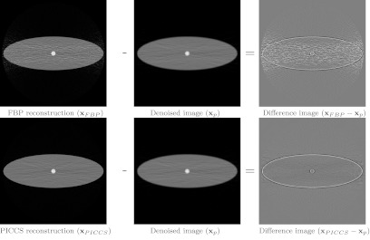
Illustration of the components contained in the difference image x − xp: edges and noise. The noise component is not as sparse as the edge component. The presence of edges in the difference images denotes that the loss in spatial resolution in xp is recovered in xFBP and xPICCS. Thus, noise is preferably mitigated and edges are mostly preserved in images processed using DR-PICCS.
In DR-PICCS applications, one central question to be addressed is to what extent can DR-PICCS recover spatial resolution from a blurred prior image. The answer to this question may depend on whether or not statistical modeling is used. In particular, the local impulse function may be anisotropic11, 12 provided that statistical modeling is used. However, the additional flexibility in generating the prior image in PICCS does offer a new opportunity to eliminate or mitigate the challenge of anisotropic spatial resolution. Namely, it is the hypothesis in this paper that this type of anisotropy could be compensated by generating the prior image using a directional denoising method. In other words, one may be able to reconstruct a DR-PICCS image with a relatively isotropic spatial resolution even when the statistical modeling is applied. In this paper, a directional diffusion filtering denoising method is studied; it is briefly reviewed in Subsection 3A.
Diffusion filtering
Anisotropic diffusion filtering is a type of image processing method based on partial differential equations (PDE). It aims at applying a spatially variant and anisotropic blur to an image. This method is used in the research presented here to reduce the noise level of the prior image used in DR-PICCS. The PDE solved in this procedure can be formally expressed as follows:41, 42, 43, 44
| (6) |
where is an M × N image, is called a diffusion tensor. The diffusion tensor C with elements Cijk describes the amount of diffusion allowed in a particular direction.
If we assume pixel sizes of Δ1 and Δ2 along horizontal and vertical directions, Eq. 6 can be written more explicitly as
| (7) |
where the discrete horizontal spatial partial derivative is given by
| (8) |
and the discrete vertical spatial partial derivative is written as
| (9) |
This discrete PDE can be solved using finite differences methods.42, 43, 44 In this scheme, the image x is a function of a “time” variable t. Different levels of diffusion are achieved by solving the equation up to different times. This results in a blurring of the image and a reduction in noise level.
Anisotropic diffusion is modeled by selecting for each spatial position k of C a real symmetric matrix whose eigenvectors describe the principal axes of diffusion. Each eigenvalue describes the diffusion rate in the direction of the associated eigenvector. When C is a factor of the 2 × 2 identity matrix at a particular spatial location k, the diffusion can be considered locally isotropic. If this is the case over the whole image, this scheme is equivalent to Perona–Malik diffusion.45 If the diffusion is isotropic and spatially uniform—i.e., for all k and k′ combinations—, the solution of Eq. 6 reduces to a Gaussian blur.
The main interest of using this approach to denoise the prior image is that it allows to select a blurring direction and amplitude based on the local structure of the object via the diffusion tensor. An interesting way of selecting the tensor is based on the local gradient of the image. An edge-preserving filter can be designed by allowing less diffusion across edges. Such a filter can be achieved using the following diffusion tensor:45
| (10) |
where [∇x]k is the local gradient at voxel k,
| (11) |
Here β is a scalar constant. It plays the role of a normalization and is selected based on the expected gradient of structures in the image. We refer to function g as diffusion coefficient. A more general expression is the following:
| (12) |
where δ and γ are scalar constants. Figure 2 shows the behavior of the diffusion coefficient for different values of δ and γ. These parameters enable one to select the amount of diffusion to be allowed for a particular local gradient value. The parameter δ controls the length of the high diffusivity plateau in the low-gradient region. It does not affect the maximum slope of the curve substantially; the slope is mainly determined by γ. Higher values of γ allow a steep transition from high to low diffusivity.
Figure 2.

Illustration of the diffusion coefficient function (g) from Eq. 12 for different values of δ and γ (a) at constant γ = 0.5 and (b) at constant δ = 2.
As is shown later in this paper, when an isotropically blurred image is used as prior image, the DR-PICCS framework with statistical weighting results in images with a lower spatial resolution in the direction perpendicular to high noise projections. However, in statistical DR-PICCS, it is possible to design a diffusion tensor C that would minimize the blurring of the prior image along a particular direction. The combination of this anisotropically filtered prior image with the statistical DR-PICCS reconstruction could lead to images with relatively isotropic spatial resolution. Specifically, one could minimize blurring along the direction of unit vector [ at a particular voxel position k by using a tensor with
| (13) |
In the numerical study, we selected the direction of vector [n]k to be perpendicular to the projection with the highest noise level intersecting voxel k. The value of parameters β, γ, and δ can be selected to offer more or less selectivity in terms of the value of the directional gradient. This enables one to optimize the diffusivity function g to minimize blurring along one direction but maximize it along another.
METHODS AND MATERIALS
This paper aimed to investigate the following hypotheses.
-
1.
DR-PICCS enables a recovery of spatial resolution to a large extent from a prior image with a degraded sharpness.
-
2.
The spatial resolution of images reconstructed using DR-PICCS behaves differently depending on the inclusion of statistical weighting.
-
3.
DR-PICCS shows an anisotropic spatial resolution when statistical weighting is used.
-
4.
The spatial resolution anisotropy depends on the amount of eccentricity present in the object.
-
5.
It is possible to design a denoising procedure for the prior image that can mitigate the spatial resolution anisotropy.
A theoretical analysis of these hypotheses would be very challenging. In this paper, we explored these issues experimentally using numerical simulations. This ensured that a ground truth was available for evaluation purpose. To evaluate the applicability of the proposed method in a real clinical situation, it is also applied to in vivo animal experimental data.
Datasets
Numerical simulations
The numerical phantom used in this study was constituted of a large elliptical disc containing a small circular disc. Several levels of eccentricity were simulated for the background ellipse. The phantom parameters are presented in Table 1. The attenuation of the background ellipse was selected to simulate soft tissue, while that of the circular structure was selected to simulate bone. The studies thus examined a high contrast situation, relevant for an evaluation of spatial resolution. Poisson distributed noise was added to each projection datum. Four hundred and forty-three projections were simulated for each of 492 view angles equally distributed over an angular range of 360°. In order to mitigate the noise in the spatial resolution measurements, 40 different noise instances were simulated for each of the four phantoms. An image matrix size of 512 × 512 with a pixel dimension of 1 mm2 was used for the reconstructions.
Table 1.
Numerical phantom parameters.
| Semimajor axes (mm) | Attenuation coefficient (mm−1) | |||||
|---|---|---|---|---|---|---|
| Phantom | Horizontal | Vertical | Background ellipse | Circle | Incident fluence (photons/detector) | |
| A | 240 | 80 | ||||
| B | 213 | 107 | 0.020 | 0.040 | 2.0 × 10⁴ | |
| C | 192 | 128 | ||||
| D | 175 | 145 | ||||
The images were reconstructed using FBP and DR-PICCS with and without statistical weighting. Two methods were used to produce the prior images: Gaussian blurring and diffusion filtering. The Gaussian blur was applied with a width parameter of 2 mm—equivalent here to the width of 2 pixels. The diffusion filtering was applied using the tensor defined in Eq. 13 with β = 0.007, δ = 2, and γ = 20. In order to illustrate the behavior of the filter in a simple case, the vector n was set to be vertical such that the blur be minimized for edges with a strong vertical gradient. The diffusion was applied with a temporal step size of 0.05 for 50 iterations, i.e., up to t = 2.5. This set of parameters is representative choice of values and was not obtained by a formal optimization procedure. An exploration of the parameter space may be an interesting research topic but is out of the scope of this paper.
In vivo datasets
The projection dataset used for this study was acquired in vivo in a porcine model. The scan was approved by the Institutional Animal Care and Use Committee (IACUC) at the University of Wisconsin–Madison. The animal was a 59 kg male swine. The mean heart rate of the swine was approximately 68 beats per minute. The scan was performed using a 64-slice GE Discovery CT scanner (GE Healthcare, Waukesha, WI) at a tube current of 50 mA, tube potential of 120 kV, and a gantry rotation period of 0.4 s. A short-scan angular range of 234.0° was used. Projection line integral data and the corresponding counts for the statistical weight D were obtained using the proprietary software provided by the vendor.
Images were reconstructed from the in vivo dataset using FBP, in addition to DR-PICCS with and without the statistical model. The prior image employed in both versions of DR-PICCS was generated by denoising the FBP image dataset using diffusion filtering. The statistical weights of matrix D were set to approximate count data obtained with the aid of the scanner's manufacturer. Because of the unavailability of a reference image and because of the difficult use of quantitative metrics, the evaluation of the in vivo dataset was done on a qualitative basis.
The noise level was matched between all implementations of DR-PICCS by reconstructing a series of images at different values of the data consistency parameter λ. The CNR was selected to be about 22 in the dorsal region of the subject for all methods used.
Evaluation metrics
Noise level
The noise standard deviation was measured over pixels within a region of interest (ROI) in an area with a uniform attenuation coefficient. In this case,
| (14) |
where
| (15) |
and NROI is the number of pixels contained within the ROI.
Spatial resolution
The potentially anisotropic behavior in spatial resolution requires the sharpness to be measured at different angles. We fitted the intensity profile along several edges with the point spread function corresponding to a Gaussian blur. We extracted the width of the corresponding blurring function, which we refer to as the pseudo-PSF width.23, 24 This metric can be measured locally in the image and can be used to evaluate the blurring of structures along several directions.
Specifically, for an image under study, x with dimension M × N, the blur was quantified as follows:
-
1.
Select a 1D linear segment ℓ through the object of interest in the image.
-
2.Solve the least squares problem
where i is the position in the image matrix, and h is a multiplicative factor. The blurred image, , is the convolution of the reference image with a normalized Gaussian function of width b. The image at 2D position (m,n) is
where Δ1 and Δ2 are the voxel dimension along the image horizontal and vertical axes. The value of b that solve the least squares problem above is used as metric of image sharpness. It is referred to as pseudo-PSF width for the rest of this paper.
An important point that must be emphasized is how to understand the width of the pseudo-PSF. The metric measures the relative blur with respect to a reference image. In the event where the image under study and the reference image do not differ in sharpness, the pseudo-PSF width takes a value at or below the voxel dimension. This observation provides a condition for a local match in spatial resolution between two images. Note that such a value could also be obtained if the image under study is sharper than the reference image.
In the numerical phantom evaluation presented in this paper, the reference image was reconstructed using FBP from a noiseless projection dataset. Thus, the evaluation using the pseudo-PSF width may only provide information about the amount of blur relative to the spatial resolution of the FBP reconstruction. It is possible but unlikely that even below the pixel width, the pseudo-PSF width retained some accuracy. This may have resulted in an anisotropic shape of the pseudo-PSF below the pixel width. However, such minute differences are not substantial. In this situation, the spatial resolution is considered to be matched with that of the reference image.
Reconstruction algorithm implementation
The FBP and PICCS algorithms were implemented using C++ with Intel Integrated Performance Primitives (IPP) libraries (Intel Corporation, Santa Clara, CA). The nonlinear conjugate gradient algorithm was used to perform the minimization of the PICCS objective function.46 The specifics of the unconstrained implementation of PICCS were described in details in the literature.24
The Gaussian blur and diffusion filter were implemented using the numerical package MATLAB (MathWorks, Nattick, MA). The diffusion filtering scheme used here was described in the literature.42, 43, 44
RESULTS
Numerical simulations: Prior images
The projection datasets corresponding to each of the 40 simulated noise instances were processed independently. An example of the prior images denoised using a Gaussian blur and the diffusion filter are presented in Fig. 3 for phantom A. One can appreciate the mitigation in noise level achieved by both methods; the CNR was 2.3 in the FBP image and approximately 24 in denoised images. The noise level of both denoised images was within 3% calculated as where σ1 and σ2 correspond to the noise standard deviation measured in each image in the ROI shown in Fig. 4.
Figure 3.

(a) shows a reconstruction of numerical phantom A using FBP. Denoised images using the Gaussian blur and the diffusion filter are also shown. These are used as prior images in DR-PICCS. The display range was set to [0.000, 0.045] mm−1. The noise level of both denoised images is within 3% calculated as . In (b), a map of the diffusion coefficient g from Eq. 13 is shown with display range [0, 1].
Figure 4.

Plots of the average noise standard deviation measured in images reconstructed using DR-PICCS without (a) and with (b) the statistical model as a function of the data consistency parameter λ [Eq. 5]. Each plot shows curves for each prior image processing methods. All measurements were performed for phantom A. The image above the plots shows the ROI where the standard deviation was measured.
While the noise level was similar in both denoised images, this was not the case with spatial resolution. The Gaussian blurred image showed a considerable loss at the edges of the circular structure at the center of the phantom. In the diffusion filtered image, the same structure remained sharp in the vertical direction but showed some blurring along the horizontal axis. A map of the diffusion coefficient is shown in Fig. 3d. On this map, darker regions are synonymous with a mitigated blurring. It is important to note that sharper edges are associated with an increase in noise in the surrounding region.
Numerical simulations: Noise level dependence on data consistency parameter
To characterize PICCS at a number of specific CNR levels, a series of values of the data consistency parameter λ from the PICCS objective function were used to reconstruct independent images. The dependence of the noise level on λ is illustrated in Fig. 4. DR-PICCS showed a similar noise level dependence on λ both with and without statistical weighting. However, the values of λ for each implementation were not matched at any particular CNR. This was expected since the matrix D = diag{n} was not normalized.
Numerical simulations: DR-PICCS without statistical weighting
The processed prior images were used in the DR-PICCS framework. The images thus generated were compared in terms of spatial resolution at a constant noise level, for each of the methods used to denoise the prior image. Images reconstructed at a constant CNR of approximately 20 using DR-PICCS without statistical weighting are presented in the left column of Fig. 5. This figure also presents polar plots of the pseudo-PSF width measured along segments at various angles.
Figure 5.

DR-PICCS reconstructions and associated pseudo-PSF width at various angles. The reconstructions shown here all had a CNR of approximately 20 in a ROI along the longest axis of the ellipse. The FBP reconstruction of this dataset [Fig. 3a] had a CNR of 2.3. The display range was set to [0.000 0.045] mm−1 for all images. The voxel width was 1 mm. Images with a pseudo-PSF width at or below the voxel width are said match the sharpness of the reference noiseless FBP image.
One can observe that the spatial resolution in images reconstructed using DR-PICCS without statistical weighting is largely restored and isotropic. The isotropy is observed for both Gaussian blurred and diffusion filtered prior images. At a CNR of 20, only a small relative loss in spatial resolution, quantified by a pseudo-PSF width of about 1.1 mm, was observed when the prior image was generated using the Gaussian blur. The pseudo-PSF was below 1 mm when the prior image was generated using the diffusion filter. The pseudo-PSF width is at or below 1 mm—the voxel width—for all cases where the CNR was 13.5 or lower. In these cases, the spatial resolution can be said to match that of the FBP reconstruction.
Numerical simulations: DR-PICCS with statistical weighting
When statistical weighting is introduced in DR-PICCS, a certain amount of spatial resolution anisotropy appeared in DR-PICCS images with a Gaussian blurred prior image. This behavior is shown in the right column of Fig. 5. At a CNR of 20, the pseudo-PSF width in DR-PICCS reconstructed images varied between 1.5 and 0.75 times the voxel width, depending on the direction along which it was measured. However, this anisotropy was largely eliminated when the prior image was generated using diffusion filtering. In that case, the pseudo-PSF width remained under 1 mm, signifying a match in spatial resolution with the FBP reconstruction.
Numerical simulations: Eccentricity dependence
Another interesting question is how the shape of the object impacts the spatial resolution properties in DR-PICCS. Figures 6789 show reconstructions of phantoms A, B, C, and D each with a different eccentricity. The CNR was constant at approximately 20 measured in the ROI shown in Fig. 4. These phantoms are constituted of a large ellipse with a semimajor axis ratios of , , , or , respectively.
Figure 6.

Pseudo-PSF width at various angles for phantom A. The reconstructions used for these measurements all had a CNR of approximately 20. The voxel width was 1 mm. Images with a pseudo-PSF width at or below the voxel width are said to match the sharpness of the reference noiseless FBP image.
Figure 7.

Pseudo-PSF width at various angles for phantom B. The reconstructions used for these measurements all had a CNR of approximately 20. The voxel width was 1 mm. Images with a pseudo-PSF width at or below the voxel width are said to match the sharpness of the reference noiseless FBP image.
Figure 8.

Pseudo-PSF width at various angles for phantom C. The reconstructions used for these measurements all had a CNR of approximately 20. The voxel width was 1 mm. Images with a pseudo-PSF width at or below the voxel width are said to match the sharpness of the reference noiseless FBP image.
Figure 9.

Pseudo-PSF width at various angles for phantom D. The reconstructions used for these measurements all had a CNR of approximately 20. The voxel width was 1 mm. Images with a pseudo-PSF width at or below the voxel width are said to match the sharpness of the reference noiseless FBP image.
Highly eccentric phantoms, such as phantom A, produce a large difference in the signal to noise ratio of vertical and horizontal projections; this effect is much less significant for more circular objects. This heteroscedasticity and the low count level in the horizontal projections may result in noise-induced streaks. These can be mitigated when the statistical model is introduced in DR-PICCS. However, this improvement comes at the cost; as discussed in Sec. 5D, the spatial resolution becomes anisotropic in images that used a Gaussian blurred prior image. It is possible to observe this behavior for all levels of eccentricity. In effect, the solid curve on the pseudo-PSF polar plots of Figs. 6789 (corresponding to the DR-PICCS reconstructions with statistical weighting and a Gaussian blurred prior image) is consistently above the voxel width in the direction perpendicular to high noise projections.
To mitigate the anisotropy, the prior image was generated using diffusion filtering. In that case, both DR-PICCS with and without statistical weighting produced images with a pseudo-PSF equal to or below the voxel width for all orientations studied. This is clearly shown on the polar plots of Figs. 6789. This result suggests that the spatial resolution of DR-PICCS matches that of the FBP reconstruction in these cases.
Another interesting observation about Figs. 6789 is that the ability of DR-PICCS to recover spatial resolution improves for less eccentric phantoms when no statistical model is used. The mechanism leading to this phenomenon is simple. More circular phantoms have projection data with a lesser maximum noise level. This enables the selection of a greater value of the data consistency parameter λ for the CNR to be maintained constant. This greater value of λ results in more consistency with the data and thus in an improved spatial resolution.
Interestingly, the recovery ability does not improve for more circular phantoms when the statistical model is included. In that case, the projection data of rays that traversed the center of the phantom were overall allocated a much lesser weight than those having passed through the edge. The ability to correct blurring at the center of the phantom is, therefore, mitigated when statistical weighting is used. This demonstrates a limitation of statistical image reconstruction. However, in the context of DR-PICCS, this situation can be improved by using a prior image reconstructed using diffusion filtering or by forgoing the statistical weights altogether. As shown above, the pseudo-PSF width in these cases is indeed near or below the voxel width of 1 mm, which signifies a match in spatial resolution with the reference FBP image.
Numerical simulations: Position dependence
The evaluations presented in Secs. 5A, 5B, 5C, 5D, 5E were all designed with the circular object at the center of the phantom. In the following experiments, three more positions were investigated: along the vertical (Fig. 10), horizontal (Fig. 11), and diagonal (Fig. 12) axes. The background ellipse was that of phantom A. As was done in previous experiments, the pseudo-PSF width was again measured at different orientations and the results were plotted in Figs. 101112.
Figure 10.

Pseudo-PSF width at various angles for phantom A with circle off-center along the vertical axis. The reconstructions used for these measurements all had a CNR of approximately 20. The voxel width was 1 mm. Images with a pseudo-PSF width at or below the voxel width are said to match the sharpness of the reference noiseless FBP image.
Figure 11.

Pseudo-PSF width at various angles for phantom A with circle off-center along the horizontal axis. The reconstructions used for these measurements all had a CNR of approximately 20. The voxel width was 1 mm. Images with a pseudo-PSF width at or below the voxel width are said to match the sharpness of the reference noiseless FBP image.
Figure 12.

Pseudo-PSF width at various angles for phantom A with circle off-center along a diagonal axis. The reconstructions used for these measurements all had a CNR of approximately 20. The voxel width was 1 mm. Images with a pseudo-PSF width at or below the voxel width are said to match the sharpness of the reference noiseless FBP image.
Overall, the results at these positions agree with those obtained when the circular structure was at the center of the phantom. Namely, the images reconstructed using DR-PICCS with the statistical model and a Gaussian blurred prior image show an anisotropic spatial resolution. This is corrected to a large extent by using the diffusion filtering method to generate the prior image. Note however that when the circle was located on the diagonal axis (Fig. 12), the direction of the peak pseudo-PSF width was slightly shifted in the clockwise direction.
In vivo datasets
The projection dataset from the animal model was processed using FBP. The FBP images were denoised using diffusion filtering to produce the prior image used in DR-PICCS. DR-PICCS reconstructions were performed with and without statistical modeling. These four images are shown in Fig. 13. Two enlarged regions are provided to allow one to appreciate the level of detail and noise in the reconstructions. The CNR measured in the dorsal region of the FBP image was 5.6; in the prior image, it was 57; and for both DR-PICCS images, it was 22.
Figure 13.

Reconstructions of the animal model dataset acquired in vivo. Three regions are shown: whole animal (left), spine and dorsal area (center), and lung (right). The display window was set to [−1000, 900] HU.
The FBP image [Fig. 13a] shows a high level of noise as expected from the tube current used for the acquisition. It is particularly noticeable in the soft tissue of the dorsal region near the spine. The texture and some of the structures of the lungs are also difficult to appreciate due to the high level of noise. The diffusion filtered image [Fig. 13b] has a much mitigated noise level with respect to the FBP image. This reduction in noise improves the detectability of low-contrast soft tissue structures in the dorsal region. However, the reduction in noise comes at the price of a loss in spatial resolution for small, low-contrast structures. This is particularly visible in the lungs where small blood vessels and airways show a clear loss in sharpness.
The DR-PICCS images reconstructed without the statistical model showed an improvement in the sharpness of structures with respect to the prior image [Fig. 13c]. This was expected from the results of the numerical studies. One can also notice the introduction of structured noise in this DR-PICCS image. This is reflected in the noise power spectrum as was demonstrated in the first publication of this series.28 All projections are weighted equally in this reconstruction scheme, which means that high noise data are allocated the same level of confidence as their low-noise counterparts. The attempt to recover spatial resolution by enforcing consistency with the data thus results in an increase in noise particularly in regions corresponding to photon-starved projections.
Finally, the DR-PICCS images reconstructed using the statistical model also showed an improvement in spatial resolution with respect to the prior image. Again this behavior is consistent with the numerical phantom study. In this case, the noise in the image is less structured and less affected by the presence of high noise projections. This is explained by the lower relative weight given to high noise projections in the reconstruction procedure. It is possible to notice that soft tissue structure in the dorsal region near the spine is more easily detected when the statistical model is used. This is consistent with the results from the first publication of this series.
Note that the presence or not of anisotropic spatial resolution is not observable for this dataset. This is a consequence of the relatively low level of eccentricity in the shape of the object, as well as the use of diffusion filtering to produce the prior image.
DISCUSSION AND CONCLUSIONS
Limitations
The numerical studies were limited in a few regards. For instance, neither a bow-tie filter nor tube current modulation were simulated. Both of these methods enable an equalization of the x-ray flux incident on the detector. This could result in less heteroscedastic projection data and thus may reduce the benefits of statistical modeling. It is also likely that the anisotropy in the spatial resolution be mitigated in that case. Furthermore, the elliptical phantoms that were used led to a difference in x-ray fluence between the vertical and horizontal axes only. This explains in part the adequate performance of the single-direction diffusion filter that was used to generate the prior image. It is possible that such a filter may not perform as well for more general objects. However, in many clinical situations, projections with low photon counts are often concentrated along a particular orientation. In such cases, the single-direction diffusion filter is expected to perform well.
Another potential limitation of the numerical studies is that only Poisson noise was simulated. Other factors such as electronic noise and scatter were not included. This should be kept in mind when comparing the results of the numerical and in vivo studies.
The in vivo study from a swine projection dataset also had some limitations. The morphology of the swine—namely, a relatively cylindrical thorax—differs from that of humans. As was demonstrated in the numerical studies, more circular objects are less affected by spatial resolution anisotropy. It is, therefore, possible that a human dataset may display this effect to a greater extent.
Conclusions
Several hypotheses were investigated in this study. It was shown that DR-PICCS may enable a fourfold reduction in noise and may recover spatial resolution to a large extent from a prior image with a degraded sharpness. However, the spatial resolution of images reconstructed using DR-PICCS behaves differently depending on the inclusion of statistical weighting. It was demonstrated that the introduction of such a model slightly limits the ability of the algorithm at correcting blurring present in the prior image. Furthermore, the use of the statistical model results in images with anisotropic spatial resolution. However, the anisotropy can be largely mitigated by using a specially designed denoising method to produce the prior image. In this work, a diffusion filtering scheme was used to this end. It is possible that other methods may provide similar advantages.
The method described in this paper could be applied to several clinical situations where low dose and high spatial resolution are necessary. In particular, the application of DR-PICCS in virtual colonoscopy is currently being investigated.
While this study was conducted in the context of DR-PICCS, its conclusions may have wider implications for statistical image reconstruction (SIR). In addition to improving scanner hardware and optimizating scanning protocols, SIR is often touted as the ultimate mean of optimizing dose in CT. As shown in this research and in Refs. 11, 12, the inclusion of a statistical model in the reconstruction procedure may, however, come at the price of anisotropic or degraded spatial resolution. In the future, this should be kept in mind when evaluating the various iterative reconstruction algorithms now being packaged with commercial CT scanners.
ACKNOWLEDGMENTS
The work is partially supported by the National Institutes of Health through R01EB009699 and R01CA169331, Varian Medical Systems, and a doctoral scholarship from NSERC-CRSNG (P.T.L.). The authors wish to thank Dr. Jie Tang, Dr. Michael Speidel, and Dr. Michael Van Lysel for their assistance with the animal study.
References
- AAPM, “AAPM position statement on radiation risks from medical imaging procedures,” PP 25–A, 2011.
- Kashyap R. and Mittal M., “Picture reconstruction from projections,” IEEE Trans. Comput. C-24, 915–923 (1975). 10.1109/T-C.1975.224337 [DOI] [Google Scholar]
- Rockmore A. J. and Macovski A., “A maximum likelihood approach to transmission image reconstruction from projections,” IEEE Trans. Nucl. Sci. 24, 1929–1935 (1977). 10.1109/TNS.1977.4329128 [DOI] [Google Scholar]
- Lange K. and Carson R., “EM reconstruction algorithms for emission and transmission tomography” J. Comput. Assist. Tomogr. 8, 306–316 (1984). [PubMed] [Google Scholar]
- Sauer K. and Bouman C., “A local update strategy for iterative reconstruction from projections,” IEEE Signal Process. 41, 534–548 (1993). 10.1109/78.193196 [DOI] [Google Scholar]
- Manglos S., Gagne G., Krol A., Thomas F., and Narayanaswamy R., “Transmission maximum-likelihood reconstruction with ordered subsets for cone beam CT,” Phys. Med. Biol. 40, 1225–1241 (1995). 10.1088/0031-9155/40/7/006 [DOI] [PubMed] [Google Scholar]
- Bouman C. and Sauer K., “A unified approach to statistical tomography using coordinate descent optimization,” IEEE Trans. Image Process. 5, 480–492 (1996). 10.1109/83.491321 [DOI] [PubMed] [Google Scholar]
- Kamphuis C. and Beekman F., “Accelerated iterative transmission ct reconstruction using an ordered subsets convex algorithm,” IEEE Trans. Med. Imaging 17, 1101–1105 (1998). 10.1109/42.746730 [DOI] [PubMed] [Google Scholar]
- Erdogan H. and Fessler J., “Ordered subsets algorithms for transmission tomography,” Phys. Med. Biol. 44, 2835–2851 (1999). 10.1088/0031-9155/44/11/311 [DOI] [PubMed] [Google Scholar]
- Thibault J., Sauer K., Bouman C., and Hsieh J., “A three-dimensional statistical approach to improved image quality for multislice helical CT,” Med. Phys. 34, 4526–4544 (2007). 10.1118/1.2789499 [DOI] [PubMed] [Google Scholar]
- Fessler J. and Rogers W., “Spatial resolution properties of penalized-likelihood image reconstruction: Space-invariant tomographs,” IEEE Trans. Image Process. 5, 1346–1358 (1996). 10.1109/83.535846 [DOI] [PubMed] [Google Scholar]
- Stayman J. and Fessler J., “Regularization for uniform spatial resolution properties in penalized-likelihood image reconstruction,” IEEE Trans. Med. Image 19, 601–615 (2000). 10.1109/42.870666 [DOI] [PubMed] [Google Scholar]
- Chen G., Tang J., and Leng S., “Prior image constrained compressed sensing (PICCS): A method to accurately reconstruct dynamic CT images from highly undersampled projection data sets,” Med. Phys. 35, 660–663 (2008). 10.1118/1.2836423 [DOI] [PMC free article] [PubMed] [Google Scholar]
- Leng S., Tang J., Zambelli J., Nett B., Tolakanahalli R., and Chen G., “High temporal resolution and streak-free four-dimensional cone-beam computed tomography,” Phys. Med. Biol. 53, 5653–5673 (2008). 10.1088/0031-9155/53/20/006 [DOI] [PMC free article] [PubMed] [Google Scholar]
- Chen G., Tang J., and Hsieh J., “Temporal resolution improvement using PICCS in MDCT cardiac imaging,” Med. Phys. 36, 2130–21305 (2009). 10.1118/1.3130018 [DOI] [PMC free article] [PubMed] [Google Scholar]
- Tang J., Hsieh J., and Chen G., “Temporal resolution improvement in cardiac CT using PICCS (TRI-PICCS): Performance studies,” Med. Phys. 37, 4377–4388 (2010). 10.1118/1.3460318 [DOI] [PubMed] [Google Scholar]
- Szczykutowicz T. and Chen G., “Dual energy CT using slow kVp switching acquisition and prior image constrained compressed sensing,” Phys. Med. Biol. 55, 6411–6429 (2010). 10.1088/0031-9155/55/21/005 [DOI] [PubMed] [Google Scholar]
- Nett B., Brauweiler R., Kalender W., Rowley H., and Chen G., “Perfusion measurements by micro-CT using prior image constrained compressed sensing (PICCS): Initial phantom results,” Phys. Med. Biol. 55, 2333–2350 (2010). 10.1088/0031-9155/55/8/014 [DOI] [PMC free article] [PubMed] [Google Scholar]
- Ramirez-Giraldo J., Trzasko J., Leng S., McCollough C., and Manduca A., “Non-convex prior image constrained compressed sensing (NC-PICCS),” Proc. SPIE 7622, 76222C (2010). 10.1117/12.837239 [DOI] [Google Scholar]
- Qi Z. and Chen G.-H., “Extraction of tumor motion trajectories using prior image constrained compressed sensing based four-dimensional Cone Beam CT (PICCS-4DCBCT): A validation study,” Med. Phys. 38, 5530–5538 (2011). 10.1118/1.3637501 [DOI] [PMC free article] [PubMed] [Google Scholar]
- Qi Z. and Chen G.-H., “Performance studies of PICCS based four-dimensional cone beam computed tomography (PICCS-4DCBCT),” Phys. Med. Biol. 56, 6709–6721 (2011). 10.1088/0031-9155/56/20/013 [DOI] [PMC free article] [PubMed] [Google Scholar]
- Ramirez-Giraldo J., Trzasko J., Leng S., Yu L., Manduca A., and McCollough C., “Nonconvex prior image constrained compressed sensing (NCPICCS): Theory and simulations on perfusion CT,” Med. Phys. 38, 2157–2167 (2011). 10.1118/1.3560878 [DOI] [PMC free article] [PubMed] [Google Scholar]
- Chen G., Thériault Lauzier P., Tang J., Nett B., Leng S., Zambelli J., Qi Z., Bevins N., Raval A., and Rowley H., “Time-resolved interventional cardiac c-arm cone-beam CT: An application of the piccs algorithm,” IEEE Trans. Med. Imag. 31(4), 907–923 (2012). 10.1109/TMI.2011.2172951 [DOI] [PMC free article] [PubMed] [Google Scholar]
- Thériault Lauzier P., Tang J., and Chen G.-H., “Prior image constrained compressed sensing: Implementation and performance evaluation,” Med. Phys. 39, 66–80 (2012). 10.1118/1.3666946 [DOI] [PMC free article] [PubMed] [Google Scholar]
- Tang J., Thériault Lauzier P., and Chen G., “Dose reduction using prior image constrained compressed sensing (DR-PICCS),” Proc. SPIE 7961, 79612K–79612K-8 (2011). 10.1117/12.878200 [DOI] [Google Scholar]
- Lubner M., Pickhardt P., Tang J., and Chen G., “Reduced image noise at low-dose multidetector CT of the abdomen with prior image constrained compressed sensing algorithm,” Radiology 260(1), 248–256 (2011). 10.1148/radiol.11101380 [DOI] [PubMed] [Google Scholar]
- Stayman J., Zbijewski W., Otake Y., Uneri A., Schafer S., Lee J., Prince J., and Siewerdsen J., “Penalized-likelihood reconstruction for sparse data acquisitions with unregistered prior images and compressed sensing penalties,” Proc. SPIE 7961, 79611L–79611L-6 (2011). 10.1117/12.878075 [DOI] [Google Scholar]
- Thérriault Lauzier P. and Chen G.-H., “Characterization of statistical prior image constrained compressed sensing. I. Applications to time-resolved contrast-enhanced CT,” Med. Phys. 39, 5930–5948 (2012). 10.1118/1.4748323 [DOI] [PMC free article] [PubMed] [Google Scholar]
- Whiting B. R., “Signal statistics in x-ray computed tomography,” Proc. SPIE 4682, 53–60 (2002). 10.1117/12.465601 [DOI] [Google Scholar]
- Tang J., Nett B., and Chen G., “Performance comparison between total variation (TV)-based compressed sensing and statistical iterative reconstruction algorithms,” Phys. Med. Biol. 54, 5781–5804 (2009). 10.1088/0031-9155/54/19/008 [DOI] [PMC free article] [PubMed] [Google Scholar]
- Candès E., Romberg J., and Tao T., “Robust uncertainty principles: Exact signal reconstruction from highly incomplete frequency information,” IEEE Trans. Inf. Theory 52, 489–509 (2006). 10.1109/TIT.2005.862083 [DOI] [Google Scholar]
- Candès E., Romberg J., and Tao T., “Stable signal recovery from incomplete and inaccurate measurements,” Commun. Pure Appl. Math. 59, 1207–1223 (2006). 10.1002/cpa.20124 [DOI] [Google Scholar]
- Donoho D., “Compressed sensing,” IEEE Trans. Inf. Theory 52, 1289–1306 (2006). 10.1109/TIT.2006.871582 [DOI] [Google Scholar]
- Rudin L., Osher S., and Fatemi E., “Nonlinear total variation based noise removal algorithms,” Physica D 60, 259–268 (1992). 10.1016/0167-2789(92)90242-F [DOI] [Google Scholar]
- Song J., Liu Q., Johnson G., and Badea C., “Sparseness prior based iterative image reconstruction for retrospectively gated cardiac micro-CT,” Med. Phys. 34, 4476–4483 (2007). 10.1118/1.2795830 [DOI] [PMC free article] [PubMed] [Google Scholar]
- Sidky E. and Pan X., “Image reconstruction in circular cone-beam computed tomography by constrained, total-variation minimization,” Phys. Med. Biol. 53, 4777–4807 (2008). 10.1088/0031-9155/53/17/021 [DOI] [PMC free article] [PubMed] [Google Scholar]
- Sidky E., Pan X., Reiser I., Nishikawa R., Moore R., and Kopans D., “Enhanced imaging of microcalcifications in digital breast tomosynthesis through improved image-reconstruction algorithms,” Med. Phys. 36, 4920—4932 (2009). 10.1118/1.3232211 [DOI] [PMC free article] [PubMed] [Google Scholar]
- Choi K., Wang J., Zhu L., Suh T., Boyd S., and Xing L., “Compressed sensing based cone-beam computed tomography reconstruction with a first-order method,” Med. Phys. 37, 5113–5125 (2010). 10.1118/1.3481510 [DOI] [PMC free article] [PubMed] [Google Scholar]
- Bian J., Siewerdsen J., Han X., Sidky E., Prince J., Pelizzari C., and Pan X., “Evaluation of sparse-view reconstruction from flat-panel-detector cone-beam CT,” Phys. Med. Biol. 55, 6575–6599 (2010). 10.1088/0031-9155/55/22/001 [DOI] [PMC free article] [PubMed] [Google Scholar]
- Ritschl L., Bergner F., Fleischmann C., and Kachelrieß M., “Improved total variation-based CT image reconstruction applied to clinical data,” Phys. Med. Biol. 56, 1545–1561 (2011). 10.1088/0031-9155/56/6/003 [DOI] [PubMed] [Google Scholar]
- Weickert J., Anisotropic Diffusion in Image Processing (Teubner, Stuttgart, 1998), Vol. 1. [Google Scholar]
- Weickert J., Romeny B., and Viergever M., “Efficient and reliable schemes for nonlinear diffusion filtering,” IEEE Trans. Image Process. 7, 398–410 (1998). 10.1109/83.661190 [DOI] [PubMed] [Google Scholar]
- Weickert J., “Coherence-enhancing diffusion filtering,” Int. J. Comput. Vis. 31, 111–127 (1999). 10.1023/A:1008009714131 [DOI] [Google Scholar]
- Weickert J. and Scharr H., “A scheme for coherence-enhancing diffusion filtering with optimized rotation invariance,” J. Visual Commun. Image Represent 13, 103–118 (2002). 10.1006/jvci.2001.0495 [DOI] [Google Scholar]
- Perona P. and Malik J., “Scale-space and edge detection using anisotropic diffusion,” IEEE Trans. Pattern Anal. Mach. Intell. 12, 629–639 (1990). 10.1109/34.56205 [DOI] [Google Scholar]
- Nocedal J. and Wright S., Numerical Optimization (Springer, New York, 1999). [Google Scholar]