Effective integration of serially presented stochastic cues

Abstract

This study examines how people deal with inherently stochastic cues when estimating a latent environmental property. Seven cues to a hidden location were presented one at a time in rapid succession. The seven cues were sampled from seven different Gaussian distributions that shared a common mean but differed in precision (the reciprocal of variance). The experimental task was to estimate the common mean of the Gaussians from which the cues were drawn. Observers ran in two conditions on separate days. In the “decreasing precision” condition the seven cues were ordered from most precise to least precise. In the “increasing precision” condition this ordering was reversed. For each condition, we estimated the weight that each cue in the sequence had on observers' estimates and compared human performance to that of an ideal observer who maximizes expected gain. We found that observers integrated information from more than one cue, and that they adaptively gave more weight to more precise cues and less weight to less precise cues. However, they did not assign weights that would maximize their expected gain, even over the course of several hundred trials with corrective feedback. The cost to observers of their suboptimal performance was on average 16% of their maximum possible winnings.

Introduction

Our perception of the world is derived from sensory measurements often referred to as cues. The challenge for an organism is to integrate the information provided by different cues to estimate important environmental properties with high precision¹. The fundamental nature of this problem is reflected in the large literature on cue integration in sensory psychology (see Jacobs, 2002; Landy, Banks, & Knill, 2011, for brief reviews) and in cognitive psychology (see Slovic & Lichtenstein, 1971, for extensive review). The most important findings have been that observers (correctly) give more weight to more precise cues and that the precision of their estimates can approach the maximum precision possible for any rule of integration.

The uncertainty or variance associated with any piece of information can have its origin outside the organism (due to environmental noise) or within the nervous system (due to sensory noise). In judging the location of a faint star, for example, one source of uncertainty is atmospheric fluctuations that affect the signal before reaching the retina, while another source of uncertainty is variance in processing the signal within the nervous system after reaching the retina. Figure 1 schematizes the factors that could potentially affect the precisions of cues (precision = reciprocal of variance) to some fixed environmental property x. The dashed line marks the division between the external world and the organism's internal sensory world. The measurement of each cue may be perturbed by additive Gaussian environmental noise ${\epsilon }_i^e$ with mean 0 and variance² $V_i^e$, additive Gaussian sensory noise ${\epsilon }_i^s$ with mean 0 and variance $V_i^s$, or both noise processes. In the general case, each cue available to the organism X_i , i = 1, … , n is perturbed by the sum³ of the two sources of noise ${\epsilon }_i^e$ + ${\epsilon }_i^s$, and this sum is itself a Gaussian random variable with mean x, variance V_i = $V_i^e$ + $V_i^s$, and precision π_i = 1/V_i. Importantly, and as shown in the Theory section, cues with higher precision should be given more weight when making an optimal decision.

Figure 1.

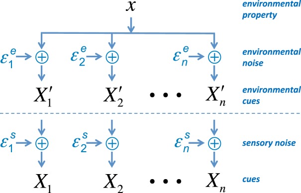
Model of factors that could potentially affect the precisions of cues. Multiple cues X_i to an environmental property x are contaminated by external environmental noise ${\epsilon }_i^e$ and by internal sensory noise ${\epsilon }_i^s$. See text for details.

This general approach to cue integration is shared across different areas of psychological research, although with slightly different emphases. While the cognitive literature tends to focus on integration of stochastic cues where the source of uncertainty is primarily external to the organism: $V_i^e$ ≫$V_i^s$, i = 1,…, n (e.g., Busemeyer, Myung, & McDaniel, 1993; Gigerenzer & Goldstein, 1996), the sensory literature tends to focus on integration of deterministic cues where the source of uncertainty is primarily internal to the organism: $V_i^s$ ≫$V_i^e$, i = 1,…, n (see Trommershäuser, Körding, & Landy, 2011). Furthermore, while cognitive studies typically address how people integrate a variable numbers of cues that are available simultaneously or sequentially, sensory studies are typically limited to how people integrate just two or three co-occurring cues.

The study presented here uses experimental techniques commonly employed in the sensory literature to investigate how people integrate seven cues presented sequentially where the source of uncertainty is primarily environmental and external to the organism. We address two key issues. First, can observers learn to give more weight to more precise cues when cues are inherently stochastic and distributed across time? Second, how does their performance compare to that of a perfectly adaptive, ideal observer who integrates cues so as to maximize the precision and expected gain of the resulting estimates?

Experimental task

The experimental task was presented using a simple cover story akin to a video game. Observers were tasked with trying to locate the best location to drill an “oil well” along a horizontal line. The true best location for the well, x, was the environmental property of interest. On each trial, observers were given seven different cues X_i , i = 1, …, 7 as to the best location for the well by seven distinct surveying companies. Each cue was presented as a tick mark that flashed briefly to indicate a spatial location along the horizontal line.

An example of the sequence of events on each trial is illustrated in Figure 2. Observers were told that the presentation order of the seven surveying companies would stay constant throughout the experiment (i.e., the first tick on each trial would always be provided by Company A, the second tick by Company B, and so on). Observers were further informed that some of the surveying companies might be better than others at estimating the best location for the well.

Figure 2.

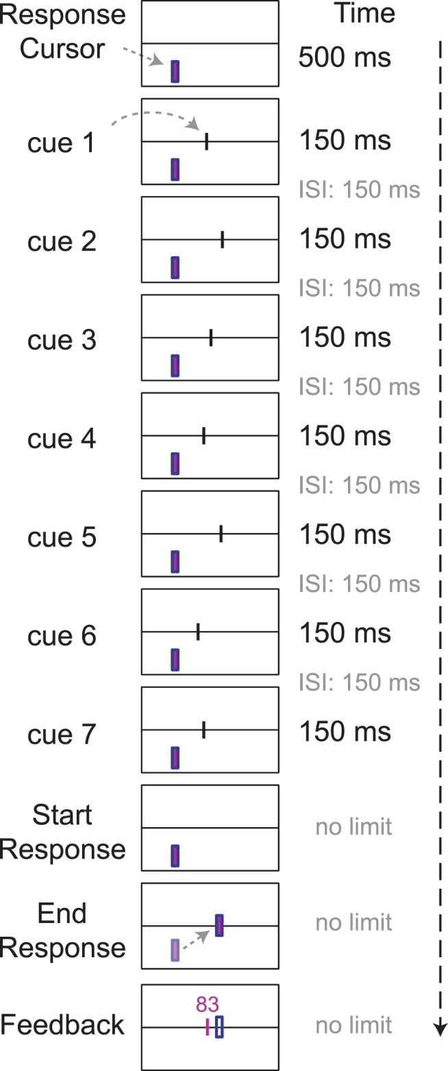
Schematic of the experimental task. The observer sees seven cues to the location of a hidden target on a horizontal line. The cues are presented one at a time, and the horizontal coordinate of each cue is drawn from a different Gaussian distribution centered on the target. After the last cue vanishes, the observer positions a response cursor to mark his estimate of the location of the hidden target. The distance between his estimate and the true location of the target determined his chances of winning a monetary reward on a random subset of the trials (see text). At the end of each trial, the observer is shown the target's location and the chances (percent) he would win the prize if the current trial were selected for reward.

The seven tick locations, or cues, were drawn from seven different Gaussians with a common mean x but with different variances V_i , i = 1, …, 7. The underlying variance of each cue was determined by presentation order. The common mean of the Gaussians (the true best location for the well) was varied at random from trial to trial. At the end of each trial, observers were provided with visual feedback indicating the true best location for the well. Observers in our study could potentially use this feedback to track the precision of each surveying company and adjust their weighting of the cues accordingly.

All observers ran in two different conditions on separate days that differed in the presentation order of the seven cues. In the decreasing precision condition, the seven cues were ordered from most precise to least precise. In the increasing precision condition they were ordered from least precise to most precise. Ultimately, the precisions of the seven surveying companies was the same in the two conditions, the only thing that changed was their presentation order.

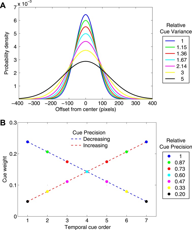
We chose to space the precision (and, therefore, the optimal weights) of the cues in a linear fashion. Figure 3A shows the probability density distributions of the seven Gaussians, and Figure 3B shows the corresponding optimal weighting function that either increases linearly or decreases linearly depending on the presentation order of the cues. Recall that, as precision is the reciprocal of variance, more precise cues have lower variance while less precise cues have higher variance.

Figure 3.

Cue precisions and optimal weights. A. The seven cues were drawn from seven different Gaussians centered on the hidden target. The probability density functions of the seven Gaussians are plotted, coded in color. The legend specifies the relative variances of the seven distributions. B. The optimal weight of each cue is proportional to its precision (reciprocal of variance). In one condition the cues were presented in order of decreasing precision, in the other, in order of increasing precision. We plot optimal cue weights versus temporal position for both conditions of the experiment. The color codes agree with those in panel A. The cue precisions and consequent variances were chosen so that the cue weights decreased and increased linearly.

While our sequential cue integration task has the same formal structure as typical sensory cue integration tasks, it differs from typical sensory tasks in important respects. Unlike typical sensory integration tasks where the source of cue uncertainty is sensory, the location cues in this task have negligible and uniform sensory uncertainty. Instead, the key imprecision of cues in this study is external to the nervous system and dictated by the experimenter. Furthermore, unlike many sensory integration tasks where there tends to be enough information in a single trial for the organism to elicit an independent estimate of the precision of each cue (Ernst & Bülthoff, 2004), in this study the precision of each cue must be learned through repeated exposures across trials. As such, we are also interested in the learning rate of cue precisions and consequent weights.

Maladaptive strategies

There are a variety of maladaptive strategies that observers might adopt for this sequential cue integration task. One possibility is that people may treat all cues equally, using the unweighted average of the cues as their estimate. This is essentially what a naïve non-learner might do if individual cue precisions were not learned across trials. In our analysis, we compared human performance to that of a hypothetical observer who assigns equal weights to the cues.

Another possibility is that, confronted with multiple cues, people may ignore most of the cues and apply a stereotypical rule to the remainder. An observer might, for example, make use of only the first few cues and ignore the rest, even when the first few cues are the least precise. Alternatively, they may choose to ignore all but the last few cues. Such a disposition to greatly overweight early or late cues would be analogous to the primacy and recency effects commonly found in memory tasks (Deese & Kaufman, 1957; Murdock, 1962). Previous work on perceptual averaging of serially presented items has found a slight recency effect with later items having greater influence on observers' estimates than earlier items (Weiss & Anderson, 1969). However, more recent work has not found evidence of differential weighting as a function of sequential presentation order (Albrecht & Scholl, 2010), especially when corrective feedback is provided throughout the experiment (Juni, Gureckis, & Maloney, 2010).

Our experiment tests for primacy and recency effects since each observer participated in both a decreasing precision condition and an increasing precision condition. If observers were simply predisposed to overweight early or late items, then we should see the same bias in both conditions.

The last possibility we consider is that people may select only one of the cues and ignore all of the remaining cues (the “veto” rule in Bülthoff & Mallot, 1988, or the “take the best” strategy in Gigerenzer & Goldstein, 1996). Even worse, the choice of which cue to follow may vary from trial to trial. In order to evaluate these possibilities, we compared human performance to an observer who uses only the single most precise cue. If participants outperform this baseline strategy, we infer that they are integrating cues effectively (Boyaci, Doerschner, & Maloney, 2006). “Effective cue integration” indicates that the observer's estimation precision exceeds that of the single most precise cue, implying that the observer is integrating information from at least two cues.

Cue integration: Theory

Unbiased cue integration

Suppose we have n independent cues to some unknown value of interest, x. Each cue X_i, i = 1, …, n is an independent Gaussian random variable with common mean x and possibly distinct variances V_i , i = 1, …, n. We define the precision of each cue to be the reciprocal of its variance π_i = 1/V_i. A more variable cue is less precise, while a less variable cue is more precise. For the purposes of our experiment, we consider a case where the cues are unbiased, independent random variables. Oruç, Maloney, and Landy (2003) consider a more general case where the cues may be correlated, while Scarfe and Hibbard (2011) consider a case where the cues may be biased.

The observer could potentially apply any rule of integration to the cues, computing any function x̂ = f(X₁, …, X_n) and taking the result x̂ to be an estimate of x (see Oruç et al., 2003). We impose one restriction, however, that the expected value of the estimate be unbiased: E[x̂] = x. Among the unbiased rules of integration, we seek the one that maximizes the precision of the resulting estimate or, equivalently, minimizes its variance.

Optimal cue integration

In the Gaussian case, the unbiased rule of integration that maximizes precision is a weighted average of the n cues

with weights w₁ + … + w_n = 1, as specified below. The resulting estimate x̂ in Equation 1 is unbiased

Moreover, since the cues are independent random variables, the precision of the resulting estimate is (Oruç et al., 2003)

where the choice of weights w_i that maximizes precision can be shown to be (Landy et al., 1995)

By substituting Equation 4 into Equation 3, we find that the precision of the resulting estimate, when integrating cues optimally, is simply the sum of the precisions of the individual cues: π(x̂) = π₁ + … + π_n. The resulting estimate must therefore have a higher precision than any of the individual cues (Oruç et al., 2003, appendix), and the ideal observer who integrates cues optimally will always achieve a greater precision than an observer who uses only one of the cues, even if it's the one with greatest precision. Any other unbiased rule of integration, linear or nonlinear, will result in estimates whose precisions are less than that of the weighted linear rule of integration in Equations 1 and 4 (Oruç et al., 2003, appendix).

A numerical example

Suppose, for example, that n = 2 and the two cues X₁ and X₂ have variances 2 and 1, respectively. Then their precisions are π₁ = 0.5 and π₂ = 1, and the optimal weights assigned by Equation 4 are w₁ = 1/3 and w₂ = 2/3. The more precise cue gets twice the weight of the less precise one. The precision of the estimate resulting from optimal cue integration is the sum of the precisions: 1.5. The variance of the resulting estimate is simply the reciprocal of the sum of the precisions: 1/1.5 = .666, which is less than that of either of the individual cues and, in fact, the lowest variance possible for any unbiased estimator.

Effective cue integration

An observer may not integrate cues optimally but still derive a benefit from integrating the cues. Suppose that in the numerical example above the observer decides to give the cues equal weight such that w₁ = w₂ = 0.5. Then the precision of the resulting estimate based on Equation 3 is:

Even though this choice of equal weights did not reach the maximum possible precision of 1.5, the observer has achieved a greater precision than could be achieved by relying on any one cue alone. Boyaci et al. (2006) refer to this sort of cue integration as effective cue integration: the precision of the observer's estimate is greater than the precision of any single cue:

We can be certain that an observer who satisfies this condition is in fact integrating cues (Oruç et al., 2003). While optimal cue integration entails effective cue integration, one can integrate cues effectively without integrating them optimally.

In this study, we compare human performance to ideal, testing whether they integrate cues with weights that achieve the maximum precision possible (optimal cue integration), and also test whether they integrate cues to achieve a greater precision than that of the most precise cue (effective cue integration).

Methods

Observers

Ten observers at New York University participated in two experimental sessions on separate days. None were aware of the purpose of the experiment and all were paid $10 per hour for their participation. Additionally, they received a performance-based monetary bonus (anywhere between $0 and $10 per session) as described below.

Apparatus

Stimuli were displayed on a 51.8 cm by 32.4 cm LCD monitor (Dell 2407WFP-HC) at a resolution of 1920 pixels by 1200 pixels with a 60-Hz refresh rate. A chin rest was used to maintain the viewing distance at 73 cm. Observers responded using the mouse and keyboard as described below. The experiment was run using MATLAB and the Psychophysical Toolbox and Video Toolbox libraries (Brainard, 1997; Pelli, 1997).

Stimulus and design

The experimental stimulus consisted of seven vertical tick marks (21 pixels high by 3 pixels wide) presented one at a time in rapid succession (150 ms duration with 150 ms spacing between ticks) drawn from seven different Gaussians that shared a common mean but had different variances. Figure 3A shows the probability density functions for the seven cues. The legend indicates the relative variance of each distribution (the standard deviations of the distributions, in pixels, and rounded to two decimal points were 61.97, 66.56, 72.36, 80.0, 90.71, 107.33, 138.56, respectively). Note that the variance of the worst cue (138.56² = 19,200) is five times greater than the variance of the best cue (61.97² = 3840). This means that the worst cue has one-fifth the precision of the best cue, and, consequently, it should ideally receive only one-fifth of the weight that the best cue receives (to maximize precision and expected gain).

Figure 3B shows the ideal weighting function for our task, which either increases or decreases linearly depending on the presentation order of the cues (increasing weights for increasing precision; decreasing weights for decreasing precision). Importantly, notice that the ideal weight assigned to each cue is the same in both conditions and that the ideal weight assigned to the most precise cue (0.2381) in both conditions is five times greater than that assigned to the least precise cue (0.0476), which, as noted above, is commensurate with their respective precisions.

The two conditions were run in separate sessions approximately two weeks apart, and their order was counterbalanced across observers. Each session lasted approximately 1 h and 20 min and consisted of 12 practice trials divided into three blocks followed by 600 experimental trials divided into 20 blocks. Observers were encouraged but not required to rest between blocks.

Procedure

Throughout the experiment, there was a horizontal reference line displayed at the center of the screen that represented the horizon along which the “oil well” could be drilled. Observers started each trial by pressing the space bar with their non-dominant hand. Upon pressing the space bar, a vertical response cursor would appear at a random location toward the bottom of the screen. Observers were prevented from adjusting the on-screen cursor until after the experimental ticks for a given trial were presented.

The location of the cursor at the start of the trial had no bearing on where the experimental ticks would appear, and we emphasized this point to the observers during the practice period. To be sure that observers were not using the random starting position of the cursor to guide their response, we checked whether there was any correlation between their final response and the initial position of the cursor. The correlation coefficient was just 0.002 and not significant. In contrast, there was a significant correlation of 0.98 between their final response and the true best location for the well, which corresponds to the common mean of the seven Gaussians from which the ticks were drawn.

As mentioned above, the common mean of the seven Gaussians was horizontally jittered from trial to trial. The jitter, which was drawn from a uniform distribution on the interval [-400,400] in pixels, was very large compared to the observers' estimation variance (with standard deviation 47.78 pixels) and to that of the spread of the seven Gaussians (maximum 138.56 pixels).

As shown in Figure 2, the first experimental tick appeared 500 ms after the start of the trial. Each tick flashed momentarily for 150 ms bisecting the horizontal reference line, and there was a 150 ms interval between flashes. Hence, the total time from the appearance of the first tick until the disappearance of the last tick was 7 × 150 ms + 6 × 150 ms = 1950 ms.

Once the last experimental tick disappeared, observers moved the cursor using their dominant hand and clicked on the reference line to mark their estimate of the best location for the well. After placing the cursor, they could make further adjustments to their estimate by right-clicking and left-clicking the mouse to move the cursor right or left one pixel at a time. They were obliged to make at least one adjustment with the mouse button even if they were content with their initial estimate. If they were content with their initial placement, they could simply click right and then left, or vice versa, to satisfy the adjustment requirement and end with their initial estimate. Once their adjustment was complete, observers pressed the space bar to record their estimate and get feedback as explained below. After receiving feedback, observers pressed the space bar again to initiate the next trial.

Monetary reward and feedback

Observers were given immediate visual feedback on each trial indicating the spatial deviation of their estimate from the true best location for the well. The response cursor was a purple tick mark surrounded by a blue rectangle. After pressing space bar to record their estimate of the best location for the well, the purple tick would change position to indicate the true best location for the well (which was at the common mean of the seven Gaussians from which the ticks were drawn), while the blue rectangle remained in place indicating the observer's estimate.

Observers were informed that they could win an extra dollar on each of 10 trials chosen at random at the end of each session. The chances of winning the extra dollar on a trial decreased by 1% for each pixel that the observer's estimate deviated from the true best location for the well. If their estimate was dead on (and the purple tick did not jump), then the chances of winning the extra dollar for that trial, if it were chosen, was 100%. If their estimate was off by 17 pixels (and the purple tick jumped 17 pixels to the right or to the left), then the chances of winning the extra dollar for that trial decreased to 83%. However, if their estimate was off by 100 pixels or more, then the chances of winning the extra dollar for that trial was 0%. Thus, observers were given an incentive to minimize the spatial deviance of their estimates from the true best location for the well, with a maximum potential reward of $10 per session.

Concurrent with the jump of the purple tick indicating the true best location for the well, an integer between 0 and 100 would appear above the purple tick indicating the chances of winning the extra dollar for that trial if it were selected for reward at the end of the session. While the observer might have trouble discriminating between being 20 pixels and 23 pixels away from the target, they should have no trouble discriminating between feedback integers that read 80 and 77, respectively.

Analysis

The following sections describe our approach to the analysis.

Cue weights

For each observer and for each condition we used linear regression to estimate the weight w_i assigned to each of the seven cues X_i using the following equation

where x̂ denotes the observer's estimate and ε ∼ Φ(0, V) is Gaussian random error with mean 0 and variance V. The error term ε captures any sensory or judgment uncertainty while the bias term captures any chronic tendency that the observer might have to aim either to the left or to the right away from the best location for the well.

For the unbiased, ideal observer who maximizes estimation precision and expected gain, the estimated weights ŵ_i, i = 1, …, 7 should show no patterned deviation from the optimal weights computed in Equation 4 and plotted in Figure 3B.

Comparing observers' cue-weights to ideal

To quantify the overall discrepancy between observers' estimated weights and the optimal weighting function, we measured the sum of the squared difference between their estimated weights ŵ_i, i = 1, …, 7 and the corresponding optimal weights w_i, i = 1, …, 7 shown in Figure 3B:

Learning cue weights

At the start of the experiment observers had no knowledge about the precisions of the cues, except that some of the cues might be better than others. We carried out the analyses on successive blocks of data to see how cue weights changed over the course of the experiment. It is of particular interest to compare observers' rate of learning in our experiment to that of an ideal learner. Because of the feedback provided at the end of each trial, an ideal learner with perfect memory would keep track of the difference between each of the seven cues $X_i^k$, i = 1,…, 7 presented on the k^th trial and the true best location for the well x^k that is given as feedback. This “perfect memory observer” could then estimate the observed precision of each cue based on the first N trials by maximum likelihood using the following equation⁴

and then update the weights of the cues using these estimated precisions in place of the true π_i in Equation 4. We computed this ideal learner by Monte Carlo simulation using 1000 runs and compared the rate of learning in this model to the learning performance of human observers.

Effective cue integration

We also compared each observer's estimation precision to that of the single most precise cue to test for effective cue integration. If their precisions are significantly greater than that of the most precise cue, we can conclude that observers indeed integrated information from more than one cue, since the only way to have a greater precision than that of the most precise cue is by integrating at least two cues (Boyaci et al., 2006; Oruç et al., 2003).

Efficiency

Finally, to quantify performance, we measured observers' efficiency, which is the ratio between their expected reward and the maximum reward possible. We computed the maximum reward of the ideal observer by Monte Carlo simulation using 1 million runs.

Results

Cue weights

Blocked analysis

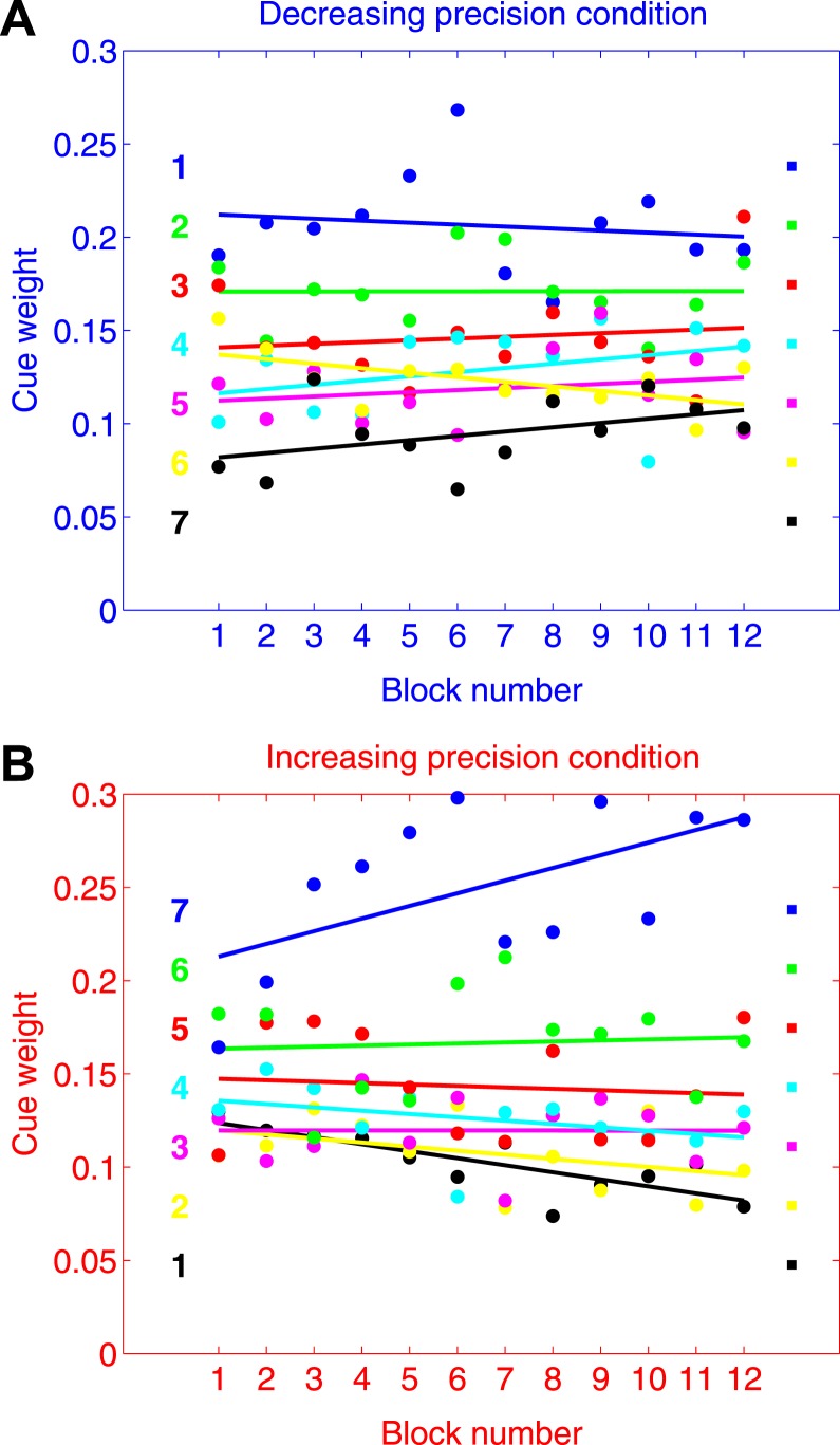
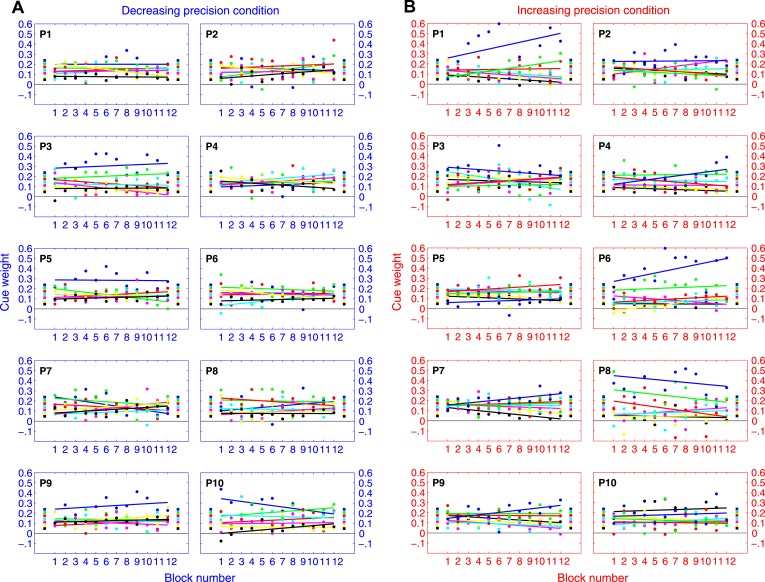
Figure 4 shows how the mean of observers' estimated weights ŵ_i for each cue changes over the course of the experiment. These weights were elicited from data in non-overlapping blocks of 50 trials. Figure 4A (blue axes) shows results for the decreasing precision condition, while Figure 4B (red axes) shows results for the increasing precision condition.

Figure 4.

Blocked analysis of cue weights (group results). A. Results for the decreasing precision condition in non-overlapping blocks of 50 trials. B. Results for the increasing precision condition in non-overlapping blocks of 50 trials. The color-coding of the seven cues follows the color scheme in Figure 3. The blue cue is the most precise one, followed by the next most precise cue in green, and so on. For reference, we placed colored squares on the right of each plot to mark the optimal weights of the cues. On the left of each plot we placed colored numerals indicating the presentation order of the cues.

There are three key observations. First, one striking aspect of the results is how little the weights changed over the course of the 12 blocks. Second, by and large, observers' estimated weights throughout the experiment were greatest for the most precise cue (blue), followed by the next most precise cue (green), and so on (irrespective of the presentation order of the cues). This indicates that observers were sensitive to differences in the precision of cues, and were able to learn very quickly the correct ordering for the weights of the cues. Finally, observers' estimated weights never quite aligned with the optimal weights of the cues. This indicates that even by the end of 600 trials, observers were unable to assign the optimal weights necessary to maximize their estimation precision. (See Figure A1 for individual results.)

Learning cue-weights and comparison to ideal

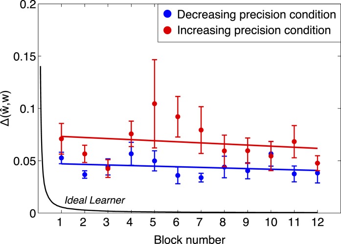
The black curve in Figure 5 shows the ideal learner's Δ(ŵ,w) (i.e., the summed squared error between the estimated cue-weights of the ideal learner and the optimal cue-weights shown in Figure 3B) as a function of number of trials observed with 95% confidence intervals. The ideal learner converges to almost optimal in fewer than 100 trials (1 block = 50 trials).

Figure 5.

Comparing trends in cue weights across time to ideal (group results). We plot the sum of the squared difference between estimated and ideal weights Δ(ŵ,w) versus block number for the decreasing precision condition (blue) and for the increasing precision condition (red). The values are averaged across observers and the error bars mark ± SEM. The black curve shows the expected convergence for an ideal learner (see text). Human performance is far from ideal even after 600 trials, and shows only a slight, non-significant trend toward convergence.

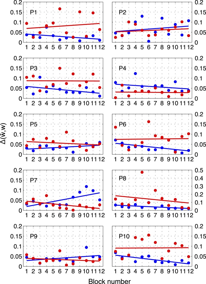
The figure also shows the mean (±SEM) of observers' Δ(ŵ,w) in non-overlapping blocks of 50 trials, separately for the decreasing precision condition (blue) and for the increasing precision condition (red). While the ideal learner converges to optimal very rapidly, observers' estimated weights did not converge to optimal even after 600 trials. We fit lines to observers' data in Figure 5 and found no significant downward trend in either condition (decreasing precision condition: t(9) = −0.53, p > 0.05; increasing precision condition: t(9) = −1.12, p > 0.05). This indicates that while observers learned very rapidly to bring Δ(ŵ,w) in the direction of optimal, they were not able to further reduce Δ(ŵ,w) as the experiment progressed, even by the end of 600 trials. (See Figure A2 for individual results.)

Given the rapid adaptation to the structure of the task, and the lack of continued learning, we focus in the remaining analyses on the last 500 trials of each condition (excluding the first 100 trials of each condition to allow for any learning at the start of each session).

Cue weights

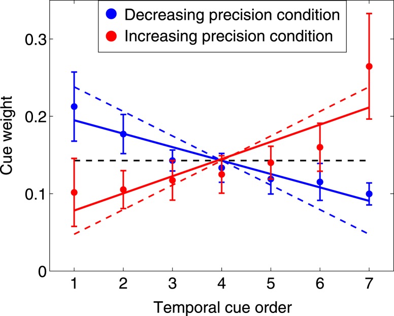
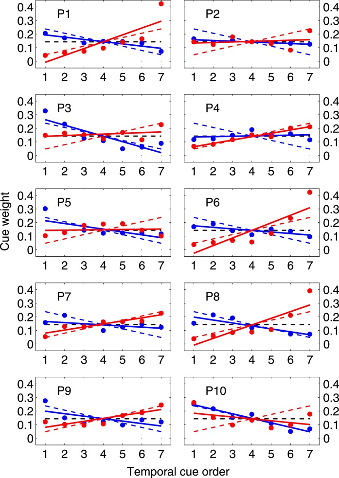
Figure 6 shows the mean and 95% CI of observers' estimated weights ŵ_i as a function of temporal cue order for the last 500 trials in each condition (decreasing precision in blue, increasing in red). The dashed lines in corresponding colors are the weights that maximize precision from Figure 3B. Optimally, the most precise cue should receive five times more weight than the least precise cue, with the intermittent cues decreasing or increasing linearly in weight depending on the condition (Figure 3B). We fit regression lines to each set of weights using the following equation

and plot the estimated fit as solid lines in blue (for decreasing precision condition) and red (for increasing precision condition).

Figure 6.

Estimated cue weights (group results). The black dashed line marks the weighting function of a hypothetical observer who gives the cues equal weights. The colored dashed lines mark the weighting function that would minimize prediction error and maximize expected gain for the decreasing precision (blue) and increasing precision (red) conditions. The dots and error bars mark the mean and 95% CI of observers' estimated weights for each of the seven cues based on the last 500 trials of each condition. The solid lines are the least squares fitted lines to observers' collective data in the corresponding condition.

While it is not always obvious from the individual results (Figure A3) that the weights follow a linear trend, the regression fits allow us to test whether there is any overall trend downward or upward in the weights. A significant negative slope indicates a downward trend while a significant positive slope indicates an upward trend. If, on the other hand, observers assigned equal weights to cues, we would expect the slopes in these linear regressions to not be significantly different from 0. The black, dashed horizontal line shows the zero slope trend line for a hypothetical observer who assigns equal weights to the cues irrespective of their precisions.

Overall, the estimated slopes m̂ of all observers' trend lines are significantly negative in the decreasing precision condition (Mean = −0.017, SD = 0.013, t(9) = −4.29, p = 0.002) and significantly positive in the increasing precision condition (Mean = 0.022, SD = 0.024, t(9) = 2.97, p < 0.05). As the slopes in both conditions were significantly different from 0, we can rule out the possibility that observers were using the unweighted average of the cues as their estimate.

Furthermore, while the estimated trend lines are not as steep as those of the ideal observer whose slope m = ±0.0317, all of the observers' estimated slopes are significantly greater in the increasing precision condition than in the decreasing precision condition, t(9) = 5.57, p < 0.001. This indicates that, on average, observers correctly assigned more weight to the more precise cues irrespective of their presentation order, though the differential weighting of the cues was not as great as the 5:1 range that is needed to be optimal.

The pooled data clearly show that observers' estimated weights trend upwards in the increasing precision condition and trend downwards in the decreasing precision conditions. This rules out the possibility that simple recency or primacy effects are responsible for the differential weighting of the cues. Instead, the group analysis indicates that observers do pick up on and exploit the differing precisions of the cues, albeit not to the full extent that is needed to be optimal.

Effective cue integration

Suboptimal but effective cue integration

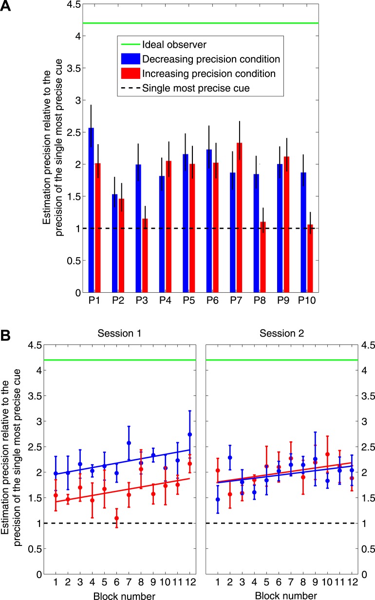
Figure 7A shows each observer's overall estimation precision for the last 500 trials of each condition compared to the precision of the single most precise cue (black dashed line) and to the maximum precision attained through optimal cue integration (green solid line). The error bars mark the 95% confidence interval of each observer's estimation precision, computed through bootstrap resampling (Efron & Tibshirani, 1993) using 10,000 runs.

Figure 7.

A. Suboptimal but effective cue integration (individual results). The choice of weights that maximizes expected gain also minimizes the variance of the weighted integration used to estimate the location of the target. We plot the precision (reciprocal of variance) of observers' estimates in each condition normalized by the precision of the single most precise cue. A value of 1 would imply that the observer's precision is no better than that of an observer who based his judgment on the single most precise cue. A value larger than 1 would imply that the observer is basing his judgment on more than one cue; i.e., he is integrating cues. We used bootstrap measures to elicit the 95% confidence interval of the precision of each observer's estimates in each condition. The green line marks the maximum possible precision of the ideal observer who integrates cues commensurate with their precisions. All observers fell short of optimal, but all exceeded the precision achievable using only the single most precise cue. Observers integrated cues effectively if not optimally. B. Blocked analysis of effective cue integration (group results). We plot the precision of observers' estimates normalized by the precision of the single most precise cue, now averaged across observers. Half the observers (P1, P3, P5, P7, P9) ran in the decreasing precision condition first (blue) while the other half ran in the increasing precision first (red). The data points mark the mean (±SEM) of each group's estimation precision in non-overlapping blocks of 50 trials. Even in the earliest blocks of each session, observers integrated cues effectively if not optimally. See text.

Overall, observers' estimation precisions were significantly greater than the single most precise cue both in the decreasing precision condition (t(9) = 11.15, p < 0.001) and in the increasing precision condition (t(9) = 4.78, p = 0.001). This indicates that observers in our task integrated cues effectively: they used more than just the single most precise cue. However their estimation precisions were significantly lower than the maximum precision of the ideal observer (who integrates all cues commensurate with their individual precisions) both in the decreasing precision condition (t(9) = −24.95, p < 0.001) and in the increasing precision condition (t(9) = −16.11, p < 0.001). Thus, they were far from integrating all cues optimally. The errors bars mark which observers in each condition were less than optimal (all observers in all conditions) and which were effectively integrating cues (all observers in the decreasing condition; all but P3, P8, P10 in the increasing condition).

Based on the relative precisions that are reported in the legend of Figure 3B, the estimation precision obtained by integrating the two most precise cues in either condition is 1 + 0.866 = 1.866. Some of the observers had estimation precisions significantly greater than that (P1 decreasing, P5 decreasing, P6 decreasing, P7 increasing, P9 increasing). The only way to obtain such high estimation precisions is by integrating at least three cues. This is the first demonstration we know of that observers effectively integrate more than two cues at a time.

Finally, we analyzed the evolution of observers' estimation precisions over the course of the entire experiment. Figure 7B shows how the precision of their estimates changes with experience. Half of the observers (P1, P3, P5, P7, P9) ran in the decreasing precision condition first while the other half ran in the increasing precision first. The data points mark the mean (±SEM) of each group's estimation precision in non-overlapping blocks of 50 trials. Observers' estimation precision gradually increased within each session (particularly in session 1). However, while there is a general trend toward improvement, observers' estimation precision is significantly lower than the maximum ideal precision of 4.2.

Efficiency

To further quantify observers' performance, we computed how efficient they were at earning bonus money. Remember that observers were instructed to make as much money as possible. Any deviation from optimal performance in learning or in integrating cues could only reduce one's expected reward. The ideal observer's chance of winning $1 on any given trial was 75.9% (SD = 18.2) once they correctly assessed cue precisions. On the other hand, the mean of observers' chances across the last 500 trials of each condition was 64% (SD = 26.89), which means that their efficiency was 0.84. Observers thus lost about 16% of all bonus money available to them. For comparison, the expected chances of an observer who made use only of the single most precise surveying company (single most precise cue) was 53.4% (SD = 31.2) for an efficiency of only 0.7. If one were to integrate the estimates of the two most precise surveying companies in an optimal fashion, one would still only obtain an expected chance of 64.3% (SD = 26.05) for an efficiency of 0.85, which is only slightly better than what observers achieved.

Discussion

We began this work by asking how observers integrate multiple pieces of visual evidence (cues) to guide their prediction of unobserved quantities in the environment. Our empirical task was designed to explore new terrain in the cue integration literature in four important ways. First, observers in our task had to integrate cues presented serially in time. This introduced a memory demand absent from previous visual cue integration work. Second, our task involved seven cues, which is more than the two to three cues typically used in sensory cue integration studies (although, larger cue sets are more commonplace in the cognitive decision-making literature, e.g., Gigerenzer & Goldstein, 1996; Slovic & Lichtenstein, 1971). Third, the precision of the cues depended on their order of presentation. In one condition the precision of successive cues decreased across a trial, in the other it increased. Successful estimation of the target property thus required observers to learn individual cue precisions across trials; they could not be assessed with any accuracy from the information provided in a single trial. Fourth, the source of uncertainty was primarily external to the sensory system. Unlike the cues in typical sensory integration tasks, there are no imperfections here in the mapping of the observed cues to the physical world. Instead, the observer's task is to estimate an unobserved parameter of the cue-generating process.

Overall, our results indicate that observers are able to (imperfectly) learn the precisions of cues across trials and integrate location cues across time in a flexible and effective manner. The majority of our observers adapted to the environmental structure of the decreasing and increasing precision of the cues. This result ruled out simple arguments concerning primacy or recency biases in the sequential processing of visual information (Deese & Kaufman, 1957; Murdock, 1962; Weiss & Anderson, 1969). Instead, our results demonstrate flexibility in how observers weight visual information when making decisions.

One study related to ours is that of van Mierlo, Brenner, and Smeets (2007). They asked observers to detect changes in slant, introducing brief delays between changes in the binocular and monocular cues defining slant. They found that observers continue to integrate monocular and binocular cues even with differences in timing up to 100 ms. However, van Mierlo et al. (2007) conclude that neural latency differences of tens of milliseconds between cues are irrelevant because of the low temporal resolution of neural processing. We, in contrast, introduce differences in timing on the order of seconds and cannot explain evidence of cue integration by low temporal resolution in neural processing.

Future investigation is needed, however, to determine whether observers' ability to learn the differential precisions of sequentially presented cues is limited to instances where cue precisions simply increase or decrease with time or whether observers can (eventually) learn more complex mappings between precision and time.

One promising direction for future research would be to determine how changes in the timing of the presentations of the tick marks affects cue integration and learning of cue precisions. If we decrease the time between ticks in a trial, do observers learn cue precisions more rapidly across trials? Or less rapidly? And, conversely, what if we increase the time between ticks? Such manipulations will allow us to characterize working memory contributions implicit in integrating discrete cues across time.

Optimal and effective cue integration

As noted in the Introduction, cue integration can meet the standard of effective (i.e., better performance than the single most precise cue) while still falling short of optimal performance. While all observers demonstrated effective cue integration, all observers fell short of optimal cue integration even after extensive training (with feedback). This result is notable since a large body of work has accumulated suggesting that human observers can integrate cues in a near-optimal fashion even without corrective feedback (Jacobs, 2002; Landy, Maloney, Johnston, & Young, 1995). Indeed, a continuing tension in the field is that studies of cognitive decision-making and learning routinely find sub-optimal performance compared to an ideal observer (Berretty, Todd, & Martignon, 1999; Gigerenzer & Goldstein, 1996; Kahneman, Slovic, & Tversky, 1982), while observers in naturalistic visual perceptual tasks show evidence of near-optimal performance (Ernst & Banks, 2002).

One interesting question is the source of this suboptimality. While the seven cues in our task were independent from one another, it is possible that limitations in working memory led to loss of cue information or introduced correlations in the representations of the objectively independent cues. If that were the case, then the expected precision of their combined estimate would be less than the sum of their individual precisions (Oruç et al., 2003). This then could potentially explain our finding of sub-optimality.

Another interesting speculation is that our finding of sub-optimality stems from the fact that the cues in our task were not simultaneously visible. Cue integration might be optimal for simultaneously accessible cues, but not for cues that are presented one at a time. This account is consistent with a bottleneck introduced via the storage or retrieval from visual short-term memory.

A final possibility is to explore these results with respect to mechanisms of sequential learning. For example, Gureckis and Love (2010) describe a model of sequential prediction in which cues are buffered in time and used to guide future prediction. Weights are learned from the memory buffer based on the predictive value of the cue for reducing prediction error (similar to a type of Rescorla-Wagner [Rescorla & Wagner, 1972], but learning through time). Such a model could provide a broad, mechanistic framework within which to explore the consequences of forgetting, selective encoding, and limitations in feedback processing that might have led to stable, suboptimal performance in the task.

Conclusion

In a sequential cue integration task using stochastic location cues, we found that people adapted their rule of integration based on the relative precisions of individual cues. This indicates that people could (imperfectly) learn the precisions of stochastic cues through repeated exposures across trials. However, performance remained well below optimal even after 600 trials with feedback. At the same time, our results found strong evidence of effective cue integration in that all observers integrated information from more than one cue in guiding their estimates. Moreover, our results are the first findings we know of to demonstrate that observers effectively integrate more than two cues at a time.

Given the many differences between our task and typical sensory cue integration tasks, we hesitate to generalize across the two kinds of tasks. Nevertheless, it is possible that maximum precision (minimum variance) cue integration is a fundamental human capability expressed across many dissimilar tasks, sensory and cognitive.

Appendix A

In this appendix we present each observer's individual results for many of the analyses that we conducted.

Figure A1.

Blocked analysis of cue weights (individual results). This figure shows the blocked results of each observer's estimated weights. This complements the group results in Figure 4.

Figure A2.

Comparing trends in cue weights across time to ideal (individual results). This figure shows the blocked results of each observer's Δ(ŵ,w) for the decreasing precision condition (blue) and for the increasing precision condition (red). Note that the y-axis for P8 is different from the rest of the observers to allow us to show an outlier point in block 5. This complements the group results in Figure 5.

Figure A3.

Estimated cue weights (individual results). This figure shows each observer's estimated weights based on the last 500 trials of each condition. The solid lines are the least squares fitted lines to each observer's data in the corresponding condition (R² across all observers and conditions ranges from 0.318 to 0.682). This complements the group results in Figure 6.

References

- Albrecht A. R., Scholl B. J. (2010). Perceptually averaging in a continuous visual world: Extracting statistical summary representations over time. Psychological Science , 21(4), 560–567 [DOI] [PubMed] [Google Scholar]
- Backus B. T., Banks M. S. (1999). Estimator reliability and distance scaling in stereoscopic slant perception. Perception , 28(2), 217–242 [DOI] [PubMed] [Google Scholar]
- Berretty P. M., Todd P. M., Martignon L. (1999). Categorization by elimination: Using few cues to choose. In Gigerenzer G., Todd P. M.the ABC Research Group. (Eds.), Simple heuristics that make us smart. (pp 235–254) New York: Oxford University Press [Google Scholar]
- Boyaci H., Doerschner K., Maloney L. T. (2006). Cues to an equivalent lighting model. Journal of Vision , 6(2):2, 106–118, http://www.journalofvision.org/content/6/2/2, doi:10.1167/6.2.2 [PubMed] [Article] [DOI] [PubMed] [Google Scholar]
- Brainard D. H. (1997). The psychophysics toolbox. Spatial Vision , 10, 433–436 [PubMed] [Google Scholar]
- Bülthoff H. H., Mallot H. A. (1988). Integration of depth modules: Stereo and shading. Journal of the Optical Society of America A , 5(10), 1749–1758 [DOI] [PubMed] [Google Scholar]
- Busemeyer J. R., Myung I. J., McDaniel M. A. (1993). Cue competition effects: Empirical tests of adaptive network learning models. Psychological Science , 4(3), 190–195 [Google Scholar]
- Deese J., Kaufman R. A. (1957). Serial effect in recall of unorganized and sequentially organized verbal material. Journal of Experimental Psychology , 54(3), 180–187 [DOI] [PubMed] [Google Scholar]
- Dodge Y. (Ed.) (2003). The Oxford dictionary of statistical terms . (p. 79). New York: Oxford University Press [Google Scholar]
- Efron B., Tibshirani R. (1993). An introduction to the bootstrap. Boca Raton, FL: Chapman & Hall [Google Scholar]
- Ernst M. O., Banks M. S. (2002). Humans integrate visual and haptic information in a statistically optimal fashion. Nature , 415, 429–433 [DOI] [PubMed] [Google Scholar]
- Ernst M. O., Bülthoff H. H. (2004). Merging the senses into a robust percept. Trends in Cognitive Sciences , 8(4), 162–169 [DOI] [PubMed] [Google Scholar]
- Gigerenzer G., Goldstein D. G. (1996). Reasoning the fast and frugal way: Models of bounded rationality. Psychological Review , 103(4), 650–669 [DOI] [PubMed] [Google Scholar]
- Gureckis T. M., Love B. C. (2010). Direct associations or internal transformations? Exploring the mechanisms underlying sequential learning behavior. Cognitive Science , 34, 10–50 [DOI] [PMC free article] [PubMed] [Google Scholar]
- Jacobs R. A. (2002). What determines visual cue reliability? Trends in Cognitive Sciences , 6(8), 345–350 [DOI] [PubMed] [Google Scholar]
- Juni M. Z., Gureckis T. M., Maloney L. T. (2010). Integration of visual information across time. Journal of Vision , 10(7):1213 [Abstract] [Google Scholar]
- Kahneman D., Slovic P., Tversky A. (1982). Judgment under uncertainty: Heuristics and biases. New York: Cambridge University Press [Google Scholar]
- Landy M. S., Banks M. S., Knill D. C. (2011). Ideal-observer models of cue integration. In Trommershäuser J., Körding K. P., Landy M. S.(Eds.), Sensory cue integration. (pp 5–29) New York, NY: Oxford University Press [Google Scholar]
- Landy M. S., Maloney L. T., Johnston E. B., Young M. (1995). Measurement and modeling of depth cue combination: In defense of weak fusion. Vision Research , 35(3), 389–412 [DOI] [PubMed] [Google Scholar]
- Murdock B. B. (1962). The serial position effect of free recall. Journal of Experimental Psychology , 64(5), 482–488 [Google Scholar]
- Oruç I., Maloney L. T., Landy M. S. (2003). Weighted linear cue combination with possibly correlated error. Vision Research , 43(23), 2451–2468 [DOI] [PubMed] [Google Scholar]
- Pelli D. G. (1997). The VideoToolbox software for visual psychophysics: Transforming numbers into movies. Spatial Vision , 10(4), 437–442 [PubMed] [Google Scholar]
- Rescorla R. A., Wagner A. R. (1972). A theory of Pavlovian conditioning: Variations in the effectiveness of reinforcement and nonreinforcement. In Black A. H., Prokasy W. F.(Eds.), Classical conditioning II: Current research and theory. (pp 64–99). New York: Appleton-Century-Crofts [Google Scholar]
- Scarfe P., Hibbard P. B. (2011). Statistically optimal integration of biased sensory estimates. Journal of Vision , 11(7):12, 1–17, http://www.journalofvision.org/content/11/7/12, doi:10.1167/11.7.12 [PubMed] [Article] [DOI] [PubMed] [Google Scholar]
- Slovic P., Lichtenstein S. (1971). Comparison of Bayesian and regression approaches to the study of information processing in judgment. Organizational Behavior and Human Performance , 6, 649–744 [Google Scholar]
- Trommershäuser J., Körding K. P., Landy M. S. (2011). Sensory cue integration. New York, NY: Oxford University Press [Google Scholar]
- van Mierlo C. M., Brenner E., Smeets J. B. J. (2007). Temporal aspects of cue combination. Journal of Vision , 7(7):8, 1–11, http://www.journalofvision.org/content/7/7/8, doi:10.1167/7.7.8 [PubMed] [Article] [DOI] [PubMed] [Google Scholar]
- Weiss D. J., Anderson N. H. (1969). Subjective averaging of length with serial presentation. Journal of Experimental Psychology , 82(1, Pt. 1), 52–63 [Google Scholar]