

Abstract
Background: Future climate change may cause air quality degradation via climate-induced changes in meteorology, atmospheric chemistry, and emissions into the air. Few studies have explicitly modeled the potential relationships between climate change, air quality, and human health, and fewer still have investigated the sensitivity of estimates to the underlying modeling choices.
Objectives: Our goal was to assess the sensitivity of estimated ozone-related human health impacts of climate change to key modeling choices.
Methods: Our analysis included seven modeling systems in which a climate change model is linked to an air quality model, five population projections, and multiple concentration–response functions. Using the U.S. Environmental Protection Agency’s (EPA’s) Environmental Benefits Mapping and Analysis Program (BenMAP), we estimated future ozone (O3)-related health effects in the United States attributable to simulated climate change between the years 2000 and approximately 2050, given each combination of modeling choices. Health effects and concentration–response functions were chosen to match those used in the U.S. EPA’s 2008 Regulatory Impact Analysis of the National Ambient Air Quality Standards for O3.
Results: Different combinations of methodological choices produced a range of estimates of national O3-related mortality from roughly 600 deaths avoided as a result of climate change to 2,500 deaths attributable to climate change (although the large majority produced increases in mortality). The choice of the climate change and the air quality model reflected the greatest source of uncertainty, with the other modeling choices having lesser but still substantial effects.
Conclusions: Our results highlight the need to use an ensemble approach, instead of relying on any one set of modeling choices, to assess the potential risks associated with O3-related human health effects resulting from climate change.
Keywords: climate change, mortality, ozone, population projections, sensitivity analysis
There is a substantial and growing literature on the potential impacts of climate change in the absence of efforts to mitigate the atmospheric accumulation of greenhouse gases due to global emissions and other factors. The recent Intergovernmental Panel on Climate Change (IPCC) Fourth Assessment Report found that “warming of the climate system is unequivocal” and that “most of the observed increase in globally averaged temperatures since the mid-20th century is very likely due to the observed increase in anthropogenic greenhouse gas concentrations” (IPCC 2007). Of particular importance for the U.S. Environmental Protection Agency’s (EPA’s) mission to protect human health and the environment is the potential for future climate change to cause air quality degradation via climate-induced changes in meteorology and atmospheric chemistry, which poses challenges to the U.S. air quality management system and the effectiveness of its pollution mitigation strategies (IPCC 2007; Isaksen et al. 2009; Jacob and Winner 2009; National Research Council 2004). In this context, the Global Change Research Program in the U.S. EPA’s Office of Research and Development, in partnership with its Office of Air and Radiation, began soliciting research that targeted the impacts of climate change on air quality in 1999 (U.S. EPA 2009a; Weaver et al. 2009).
To move from a consideration of environmental impacts to an explicit assessment of human health risks, the demographics, and the size of the exposed population, whether now or in the future, is a critical input to any analysis of the human health effects related to climate change. Therefore, the U.S. EPA has concurrently been developing high-resolution, spatially explicit population projections for the United States. These projections, from the Integrated Climate and Land-Use Scenarios (ICLUS) project (U.S. EPA 2009b), have been developed to be consistent with the underlying assumptions of the IPCC Special Report on Emissions Scenarios (SRES) social, economic, and demographic storylines (Nakicenovic et al. 2000; U.S. EPA 2009b).
Our work builds on these two efforts by examining the potential indirect impacts of climate change on the health of a hypothetical future U.S. population [in approximately (ca.) year 2050] via its direct impact on tropospheric ozone (O3) concentrations. We input both the results of the linked climate change and air quality models (hereafter referred to as the climate change–air quality modeling systems) and various population projections into the Environmental Benefits Mapping and Analysis Program (BenMAP), the U.S. EPA’s air pollution benefits analysis model, to estimate the changes in adverse health effects resulting from the changes in ambient O3 concentrations simulated by the climate change–air quality modeling systems. Our analysis considers the health impacts associated with O3 changes induced only by future climate change; the air quality modeling simulated the response of O3 to global climate change alone, without changes in anthropogenic emissions of O3 precursors [e.g., due to future air quality management efforts and future economic growth, as described previously (U.S. EPA 2009a; Weaver et al. 2009)].
In several studies, investigators modeled the health impacts of climate change–induced changes in O3 (Bell et al. 2007; Hwang et al. 2004; Knowlton et al. 2004; Sheffield et al. 2011; Tagaris et al. 2009; West et al. 2007). All of these studies found that simulated climate change produced increases in O3-related mortality. Tagaris et al. (2009) also found the potential for additional PM2.5-related mortality due to climate change. However, few studies have investigated the sensitivity of their estimates to the underlying modeling choices. For example, each of the references cited used a single climate change–air quality modeling system as the basis for their analysis, although Tagaris et al. (2009) did provide a useful estimate of the uncertainty surrounding their O3-related health findings based on the range of results reported in Weaver et al. (2009). Similarly, only West et al. (2007) considered population growth in their analysis. Therefore, instead of developing a quantitative estimate of future human health impacts of climate-induced O3 changes, our goal, building on these previous studies, was to assess the sensitivity of such estimates to key modeling assumptions and choices. Our purpose was to explore the uncertainty surrounding the assessment of these climate-related health impacts and to sketch out the set of health risks that society must begin to consider.
Methods
Our study was designed to assess the sensitivity of projected future O3-related human health impacts in the United States to modeling and methodological choices for a) climate-induced changes in future meteorological conditions; b) the changes in O3 concentrations resulting from those meteorological changes; c) the size of the affected population, as well as its age and geographic distributions; and d) the concentration–response (C–R) relationships linking O3 levels to specific health outcomes.
There is substantial uncertainty surrounding each of the inputs to our analysis, particularly because it focuses so far into the future. Much of this uncertainty cannot be assessed quantitatively. Even assigning probabilities to the different models (representing our subjective assessments about the relative accuracy with which each approximates a future reality) is premature. Instead, we present our analysis as a series of sensitivity analyses or “what if” scenarios designed to assess the impact of the various assumptions and modeling approaches on the results. Figure 1 illustrates the basic structure of the analysis.
Figure 1.

The structure of the analysis of O3-related impacts on human health attributable to climate change. GHG, greenhouse gas.
Climate change–air quality modeling systems. Our analysis includes seven modeling efforts of six research groups: Harvard University; Carnegie Mellon University (CMU); Washington State University (WSU); U.S. EPA’s National Exposure Research Laboratory (NERL); the joint efforts of the Georgia Institute of Technology, the Northeast States for Coordinated Air Use Management, and the Massachusetts Institute of Technology (GNM); and the University of Illinois, which considered two different SRES scenarios (denoted Illinois-1 and Illinois-2), but otherwise used identical setups. The Harvard and CMU simulations used global-scale (e.g., 4° × 5° grids) atmospheric chemistry models. The remaining simulations used regional air quality models, which necessitates downscaling global climate model data to fine scales (e.g., 36-km grids). These modeling efforts are described in detail elsewhere (U.S. EPA 2009a; Weaver et al. 2009); we have summarized the key characteristics in Tables 1 and 2. Briefly, each modeling group explored the potential impacts of climate change on O3 concentrations in the United States using two linked models. First, we used a climate model to simulate meteorological conditions in the United States for future years (under climate change) and in the present. This modeled meteorology was then input to an air quality model to simulate the ambient O3 concentrations that would result. Anthropogenic emissions were held constant between the base case and the climate change case, but climate-sensitive biogenic and evaporative emissions were allowed to change in response to changes in climate. Baseline emissions were similar, although not identical, across modeling efforts (e.g., for the United States, based largely on 1999 or 2001 U.S. EPA emissions inventory data), as detailed in the references cited by the U.S. EPA (2009a) and Weaver et al. (2009). Some modeling groups used dynamical downscaling (with a regional climate model) to further regionalize the global climate model simulation outputs. The choice of downscaling model and methodology is an additional source of uncertainty, but systematically separating out this additional source was not feasible for this analysis.
Table 1.
Summary of global climate and O3 modeling systems used in this analysis.
| Modeling system | Harvard | CMU | ||
|---|---|---|---|---|
| Simulation period | 5 summers/falls | 10 summers/falls | ||
| GCM | GISS III | GISS II’ | ||
| Resolution | 4° × 5° | 4° × 5° | ||
| GHG scenario | A1b | A2 | ||
| GCTM | GEOS-chem | GISS II’ | ||
| Climate sensitive emissions | BVOCs; lightning and soil NOx | BVOCs; lightning and soil NOx | ||
| Abbreviations: A1b, A2, the names given to the SRES scenarios of greenhouse-gas (GHG) emissions used to drive the climate models; BVOC, biogenic volatile organic compounds; GCM, general circulation model; GCTM, global chemical transport model; GEOS, Goddard Earth Observing System; GISS, Goddard Institute for Space Studies; NOx, nitrogen oxides. | ||||
Table 2.
Summary of regional climate and O3 modeling systems.
| Modeling system | NERL | Illinois-1 | Illinois-2 | WSU | GNM | |||||
|---|---|---|---|---|---|---|---|---|---|---|
| Simulation period | 5 JJAs | 4 JJAs | 4 JJAs | 5 Julys | 3 JJAs | |||||
| GCM | GISS III | PCM | PCM | PCM | GISS III | |||||
| Global resolution | 4° × 5° | 2.8° × 2.8° | 2.8° × 2.8° | 2.8° × 2.8° | 4° × 5° | |||||
| GHG scenario | A1b | A1Fi | B1 | A2 | A1b | |||||
| RCM | MM5 | CMM5 | CMM5 | MM5 | MM5 | |||||
| Regional resolution | 36 km | 90/30 km | 90/30 km | 36 km | 36 km | |||||
| Convection scheme | Grell | Grell | Grell | Kain–Fritsch | Grell | |||||
| RAQM | CMAQ | AQM | AQM | CMAQ | CMAQ | |||||
| Chemical mechanism | SAPRC99 | RADM2 | RADM2 | SAPRC99 | SAPRC99 | |||||
| Climate sensitive emissions | BVOCs; evaporative | BVOCs; evaporative | BVOCs; evaporative | BVOCs; evaporative | BVOCs; evaporative | |||||
| Abbreviations: A2, A1b, A1Fi, B1, and B2, the names given to the SRES scenarios of greenhouse-gas (GHG) emissions used to drive the climate models; AQM, air quality model; BVOC, biogenic volatile organic compounds; CMAQ, Community Multiscale Air Quality Model; CMM5, University of Illinois climate extension of the Penn State/National Center for Atmospheric Research (NCAR) Mesoscale Model, version 5; GCM, general circulation model; GISS, Goddard Institute for Space Studies; JJA, June, July, August; Grell and Kain-Fritsch, convective parameterizations in the regional climate models; MM5, Penn State/NCAR Mesoscale Model, version 5; PCM, parallel climate model; RADM2, Regional Atmospheric Deposition Model (2nd generation); RAQM, regional air quality model; RCM, regional climate model; SAPRC, statewide air pollution research center; SAPRC99, one of the chemical mechanism packages used in the CMAQ model. | ||||||||||
The modeling groups produced from 3 to 10 summers of maximum daily 8-hr average ozone concentrations (MDA8) that were approximately centered on the years 2000 (present) and 2050 (future). The MDA8 was computed by taking rolling 8-hr averages for a 24-hr period and then taking their maximum. This was performed for all days in the modeled O3 seasons. Although different models used different grids, the air quality grids for all of the models were remapped to a 30 km × 30 km grid for this analysis for consistency. Further adjustment of modeled air quality is described in Supplemental Material, p. 3 (http://dx.doi.org/10.1289/ehp.1104271).
Population projections to a future year. All of the BenMAP runs used populations projected to 2050. To explore the sensitivity of our results to assumptions about what this future population would look like, we selected five population projections for input into our analysis. One of these was simply the 2000 Census population (i.e., we assumed no change from the 2000 Census population by 2050 to show the risk associated with climate change in the absence of changes in populations exposed) (U.S. EPA 2010b). A second population projection is extrapolated from the Woods & Poole population projections for the year 2030 already in BenMAP (Woods & Poole Economics Inc. 2007), using a set of exponential smoothing forecasting methods [for details, see Supplemental Material, pp. 3–4 (http://dx.doi.org/10.1289/ehp.1104271)]. Finally, we selected three of the ICLUS population projections—A1, A2, and the base case—to provide the lower and upper bound ICLUS total population projections, as well as an intermediate case. The basis for the ICLUS population projects and the underlying assumptions are described in detail elsewhere (U.S. EPA 2009b) and more briefly in the Supplemental Material, p. 4.
C–R relationships and health impact functions. We followed the selection of health effects, studies, and C–R functions that the U.S. EPA used in the benefits analysis for the Regulatory Impact Analysis of the National Ambient Air Quality Standards for O3, which was completed in 2008 (U.S. EPA 2008; 2010a). The C–R functions are taken from epidemiological studies, and we assumed they were applicable to any year, although this assumption entails additional uncertainties. The suite of health effects included mortality from all causes (all-cause mortality), nonaccidental mortality, hospital admissions for respiratory illnesses, emergency room (ER) visits for asthma, school loss days; and minor restricted activity days [see Supplemental Material, Table S1 (http://dx.doi.org/10.1289/ehp.1104271) for study details]. For several health effects, two or more C–R functions were pooled (see Supplemental Material, pp. 4–5 for details on pooling and Table S4 for the pooled estimates).
Most of the studies in the air pollution epidemiological literature have estimated exponential (log-linear) C–R functions in which the natural logarithm of the health effect is a linear function of the air pollutant:
y = Beβx, [1]
where x is the ambient air pollutant (e.g., O3) level, y is the incidence of the health effect at O3 level x, β is the coefficient of ambient O3 concentration, and B is the incidence at x = 0.
The health impact function—the relationship between a change in the pollutant concentration (Δx = x1–x0) and the corresponding change in incidence of the health effect in the population (Δy = y1–y0)—derived from the log-linear C–R function is
Δy = y0[eβΔx–1], [2]
where x1 and x0 represent the model-simulated summertime O3 levels ca. 2050 and ca. 2000, respectively, while y1 and y0 represent the health effect incidence in the with and without climate-change (baseline) scenario, respectively. The baseline incidence (y0) is the product of the baseline incidence rate and the exposed population. The measure of O3 concentration available from the climate change–air quality models is the O3 season average of the MDA8. The C–R functions relate the MDA8 to health effects, and we applied this O3 season average MDA8 to each day. Because the health impact functions are nearly linear, this application of a seasonal average to each day in the season provides a good approximation to the result we would get if we had individual daily 8-hr maxima for each day in the O3 season. In many cases, the C–R function used an O3 metric other than the MDA8 (e.g., the 24-hr mean) [see Supplemental Material, Table S1 (http://dx.doi.org/10.1289/ehp.1104271)]; the coefficients from these functions were converted to coefficients for the MDA8 (for the methods, see Abt Associates Inc. 2010, Appendix G). This conversion would be expected to add only a small amount of uncertainty to the results.
Baseline incidence rates. A detailed description of the estimation of baseline incidence rates ca. 2050 is given in the Supplemental Material, pp. 5–7 (http://dx.doi.org/10.1289/ehp.1104271). Briefly, we calculated cause-specific death counts at the county level for selected age groups from individual-level mortality data for years 2004 through 2006, obtained from the Centers for Disease Control and Prevention (CDC 2008b), National Center for Health Statistics (NCHS), for the entire United States. The county-level death counts were then divided by the corresponding county-level population to obtain the mortality rates. We used 3 years (2004–2006) of mortality and population data to provide more stable estimates. We then extrapolated these county-level mortality rates to 2050 using the U.S. Census Bureau national mortality life tables (U.S. Census Bureau 2010).
Regional rates for hospitalizations and asthma ER visits were calculated from year 1999 regional hospitalizations and year 2000 ER visits obtained from the National Hospital Discharge Survey and the National Hospital Ambulatory Medical Care Survey, respectively (CDC 2008a, 2010) [see Supplemental Material, pp. 6–7 (http://dx.doi.org/10.1289/ehp.1104271)]. We applied the regional rates to every county in a region. Hospitalization rates are cause specific, with causes defined by those combinations of the International Classification of Diseases, Ninth Revision (ICD-9) codes (see Supplemental Material, Table S1) that were used in the selected epidemiological studies (e.g., Bell et al. 2004; Ito et al. 2005). However, we were unable to project rates of hospitalizations and ER visits to 2050 because, unlike mortality rates, there are no reliable projections of rates for hospitalizations or for ER visits or for trends into the future.
Defining the O3 season. The climate change–air quality models used in this analysis generally defined the O3 season as June, July, and August (i.e., climatological summer in the Northern Hemisphere). Although most of the air pollution epidemiology studies that have focused on O3 have defined the season more broadly (e.g., May through September), we used the more conservative June through August definition for consistency with the O3 simulations. Modeling results summarized in Weaver et al. (2009) indicate similar magnitudes of climate-induced O3 increases in fall and spring, suggesting that the health impacts we report here are more conservative than if we considered a more standard, longer O3 season.
Estimation of human health impacts. BenMAP calculated the change in each adverse health effect within each grid cell of the air quality grid by combining the appropriate C–R function coefficient (β), baseline incidence (y0), and simulated change in O3 due to climate change (Δx) in the health impact function (Equation 2). Although BenMAP uses the same “national” C–R function coefficient (β) in all grid cells, population estimates and baseline incidence rates in the health impact function are as location-specific as possible. The grid cell-specific changes in health effects are then summed across grid cells to produce county-level, state-level, and national estimates of health impacts.
Results
Using the 7 climate change–air quality modeling systems and the 5 population projections, we produced 35 potential answers to the question: How many O3-related cases of a given health effect (e.g., nonaccidental mortality) may be attributable to climate change in the conterminous United States in a future year? We also considered more than one C–R function for some health effects, further increasing the number of potential answers.
National results. Estimates of the annual national O3-related nonaccidental mortality ca. 2050 ranged from > 600 deaths avoided because of climate change to > 2,500 deaths attributable to climate change, depending on the climate change–air quality modeling system, population projection, and C–R function used (Table 3). Estimates for all-cause mortality follow similar patterns according to the climate change–air quality modeling system and population projection [see Supplemental Material, Table S2 (http://dx.doi.org/10.1289/ehp.1104271)]. The broad patterns seen for mortality across the different modeling choices are largely mirrored for the morbidity effect estimates as well, though for some health outcomes the numbers of cases are much larger, for example, in the hundreds of thousands or millions for minor restricted activity days (see Supplemental Material, Tables S3–S7).
Table 3.
Estimated changes in national summertime (June–August) O3-related nonaccidental mortality due to simulated climate change between 2000 and ca. 2050.a
| Modeling system | Study | Population projection | ||||||||||
|---|---|---|---|---|---|---|---|---|---|---|---|---|
| ICLUS-A1 | ICLUS-A2 | ICLUS-BC | W&P | Census 2000 | ||||||||
| Illinois-1 | Bell et al. 2004 | 570 | 520 | 510 | 440 | 170 | ||||||
| Ito et al. 2005 | 2,560 | 2,340 | 2,280 | 1,970 | 780 | |||||||
| Schwartz 2005 | 860 | 790 | 770 | 670 | 270 | |||||||
| Illinois-2 | Bell et al. 2004 | 530 | 480 | 480 | 420 | 160 | ||||||
| Ito et al. 2005 | 2,390 | 2,180 | 2,160 | 1,870 | 710 | |||||||
| Schwartz 2005 | 810 | 730 | 730 | 640 | 250 | |||||||
| CMU | Bell et al. 2004 | 480 | 430 | 430 | 350 | 150 | ||||||
| Ito et al. 2005 | 2,180 | 1,950 | 1,920 | 1,570 | 690 | |||||||
| Schwartz 2005 | 730 | 660 | 650 | 540 | 240 | |||||||
| Harvard | Bell et al. 2004 | 240 | 220 | 230 | 200 | 80 | ||||||
| Ito et al. 2005 | 1,090 | 1,000 | 1,030 | 890 | 380 | |||||||
| Schwartz 2005 | 370 | 340 | 350 | 300 | 130 | |||||||
| GNM | Bell et al. 2004 | 40 | 30 | 20 | 10 | –20 | ||||||
| Ito et al. 2005 | 180 | 140 | 80 | 50 | –80 | |||||||
| Schwartz 2005 | 60 | 50 | 30 | 20 | –30 | |||||||
| NERL | Bell et al. 2004 | 10 | 10 | –10 | –50 | –20 | ||||||
| Ito et al. 2005 | 50 | 20 | –40 | –240 | –100 | |||||||
| Schwartz 2005 | 20 | 10 | –20 | –80 | –40 | |||||||
| WSU | Bell et al. 2004 | –150 | –140 | –110 | –60 | 0 | ||||||
| Ito et al. 2005 | –650 | –630 | –480 | –240 | 0 | |||||||
| Schwartz 2005 | –220 | –210 | –160 | –90 | 0 | |||||||
| W&P, Woods & Poole. aNumbers rounded to the nearest 10. | ||||||||||||
Figure 2 summarizes the influence of the climate change–air quality modeling system and population projection on estimates of future O3-related nonaccidental deaths attributable to climate change, using the C–R function described by Bell et al. (2004). The C–R function is itself a source of substantial uncertainty. For example, had we used the C–R function described by Ito et al. (2005) instead, the numbers would have generally been more than 4 times larger (e.g., 2,560 attributable deaths compared with 570 based on Illinois-1 and ICLUS-A1), although the basic pattern according to climate change–air quality modeling system and population projection is the same (Table 3).
Figure 2.
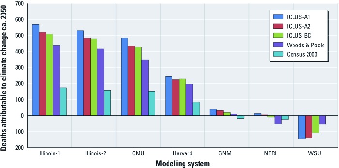
Estimated national summertime (June–August) O3-related nonaccidental mortality due to simulated climate change between 2000 and ca. 2050 (C–R function from Bell et al. 2004). We estimated that –0.6 deaths were based on the WSU climate change model–air quality model and Census 2000 population data.
Our analysis is one of the first to account for population growth and associated changes in age and geographic distributions. We found that considering these factors has a substantial influence on the estimates of health impacts. The assumption that the population ca. 2050 will be exactly what it was in the year 2000 (i.e., by using Census 2000 population estimates) produces estimates that are consistently lower than those based on population projections, all of which assume at least some increase in population size relative to the year 2000, in addition to changes in the age distribution of future populations, as shown in Figure 2 and Table 3 (and proposed by Tagaris et al. 2009).
The choice of methods to project future age and geographic distributions can also influence results. For example, although the ICLUS-A2 population projection for 2050 is, in total, greater than the ICLUS-A1 projection (424.8 million vs. 386.7 million), ICLUS-A1 is skewed more toward the older age groups [with about 26% projected to be ≥ 65 years of age in 2050 versus only about 21% based on ICLUS-A2; see Supplemental Material, Figure S1 (http://dx.doi.org/10.1289/ehp.1104271)]. Because older people have substantially higher baseline incidence rates for mortality (and other adverse health effects) than do younger people, the same increase in O3 concentration would result in more deaths among an older population than among a younger one because the estimated change in the outcome is a function of the baseline incidence, which is the product of the baseline incidence rate and the population size. This is reflected in the slightly higher numbers of O3-related deaths for ICLUS-A1, despite the overall smaller population. If C–R functions were available for age group-specific mortality, their application would likely accentuate the importance of age distribution, because older people may be more vulnerable to air pollution.
The importance of the age distribution of the affected population is particularly apparent when we consider morbidity effects that focus on specific age subgroups in the population, such as O3-related school days lost (5–17 years of age) or respiratory hospital admissions among those ≥ 65 years of age [see Supplemental Material, Tables S3, S4, S6, S7 (http://dx.doi.org/10.1289/ehp.1104271)]. For example, estimates of O3-related respiratory hospital admissions among infants attributable to climate change for a year ca. 2050 based on the ICLUS-A1 population projection are uniformly smaller in magnitude than are the corresponding estimates based on ICLUS-A2 regardless of the climate change–air quality modeling system used (see Supplemental Material, Table S3). This is because ICLUS-A2 projects that a greater percentage of the population (and a larger total population) will be < 1 year of age, and that a smaller percentage of the population will be ≥ 65 years of age, relative to ICLUS-A1 (see Supplemental Material, Figure S1).
Across all of these dimensions, the source of the greatest uncertainty, for both nonaccidental and all-cause mortality, appears to be the projections of future climate change-induced meteorological changes and corresponding air quality changes, which are determined by the climate change–air quality modeling system used. This is shown clearly in the results of an analysis of variance, which decomposes the total variability in estimated mortality into the variability due to the chosen climate change–air quality modeling system, population projection, epidemiological study (C–R function) used, and interactions between these modeling choices, respectively (see Table 4). The different impacts across modeling choices are magnified to a greater or lesser degree by study choice (i.e., by C–R function) [see Supplemental Material, Figure S2 (http://dx.doi.org/10.1289/ehp.1104271)].
Table 4.
Analysis of variance results for estimates of national summertime (June–August) O3-related nonaccidental mortality due to simulated climate change between 2000 and ca. 2050.
| Source | df | ANOVA SS | Percent of total SS | |||
|---|---|---|---|---|---|---|
| Modeling system | 6 | 24,271,499 | 48 | |||
| Population projection | 4 | 2,108,558 | 4 | |||
| Study | 2 | 9,055,636 | 18 | |||
| Modeling system × study | 12 | 10,495,284 | 21 | |||
| Modeling system × population projection | 24 | 2,641,882 | 5 | |||
| Study × population projection | 8 | 921,745 | 2 | |||
| Modeling system × study × population projection | 48 | 1,165,135 | 2 | |||
| Total | 104 | 50,659,739 | 100 | |||
| Abbreviations: df, degrees of freedom; SS, sum of squares. | ||||||
Regional estimates. Because national estimates can mask very different regional changes, we delineated three broad regions for additional analysis: the Northeast (defined as east of 100° west longitude and north of 36.5° north latitude); the Southeast (defined as east of 100° west longitude and south of 36.5° north); and the West (defined as everything west of 100° west longitude). These three regions account for the entire continental United States. Finer-scale regional breakdowns, while possible, would have been an overinterpretation of our results given the various uncertainties.
Figure 3 shows national and regional estimates of O3-related nonaccidental mortality using the C–R function from Bell et al. (2004) and the ICLUS-A1 population projection, and it illustrates this national-level masking of differing regional trends. For example, the modest net change in nationwide O3-related nonaccidental mortality based on the WSU climate change–air quality modeling system represents the sum of highly variable regional estimates (i.e., 275 avoided deaths in the Northeast, plus 369 additional deaths in the Southeast, plus 54 additional deaths in the West). With the exception of Illinois-1 and Illinois-2, none of the driving climate–air quality scenarios produces regional health impact estimates that are all in the same direction [i.e., increases in the estimated O3 concentrations attributable to climate change in some regions are accompanied by decreases in other regions, due, for example, to factors such as differences in circulation patterns and increases in cloud cover (see Weaver et al. 2009)]. Although the WSU climate change–air quality simulation estimates suggest large decreases in O3-related deaths in the Southeast and large increases in the Northeast, the GNM and NERL model estimates show regional effects in just the opposite directions. These same general patterns are evident for all-cause mortality and for different C–R functions for either type of mortality.
Figure 3.
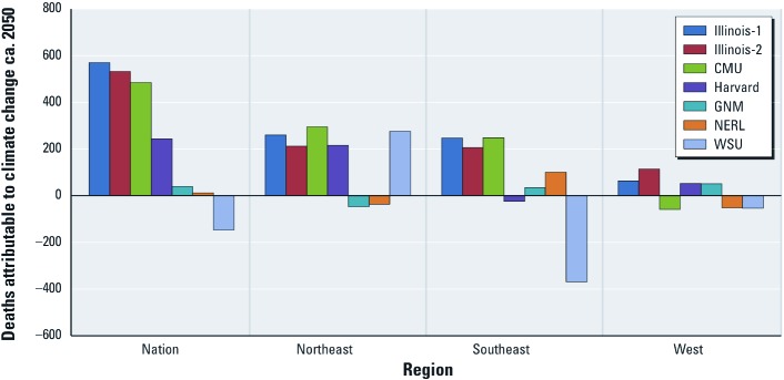
Estimated national and regional summertime (June–August) O3-related nonaccidental mortality due to simulated climate change between 2000 and ca. 2050 (C–R function from Bell et al. 2004; ICLUS-A1 population projection).
Discussion
We have attempted to assess the sensitivity of estimated O3-related human health effects of climate change to the following key modeling assumptions and choices: a) climate-induced changes in meteorological conditions and the corresponding changes in O3 concentrations; b) projections regarding the size, and age and geographic distributions of the affected population; and c) the C–R relationships linking O3 levels to specific health outcomes.
Looking across all combinations of modeling choices (including the climate change–air quality modeling system, population projection, and C–R relationship), estimates of national O3-related mortality and morbidity attributable to climate change by mid-century span a wide range (e.g., from roughly 600 cases of nonaccidental mortality avoided as a result of climate change to roughly 2,500 cases attributable to climate change).
The source of the greatest uncertainty at the national level appears to be the climate change–air quality scenario used, with choice of C–R function and population projection also important, though less influential in this analysis. Not only is the total population exposed to O3 in a future year important, but assumptions regarding the age distribution of that population are also important for estimating O3-related adverse health effects. The variability of these estimates represents the true extent of uncertainty in the problem, however, only to the extent that our choices (seven simulations, five population projections, a few alternative C–R specifications, and a single unchanging set of emissions to air) span the full range of possibilities in their respective dimensions. Thus, our estimates may understate the plausible range of potential future outcomes.
National results can mask important regional differences. Estimates for the Northeast region generally indicated adverse health impacts and were the most consistent across the seven climate–air quality scenarios of the three regions. In contrast, estimated health impacts for the Southeast showed substantial variation. The West generally showed the smallest impacts, largely due to the relatively smaller projected populations.
The wide range of estimated O3-related mortality and morbidity attributable to climate change resulting from different methodological choices highlights the need to consider an ensemble of estimates, rather than relying on any one modeling system or set of assumptions. Despite this range, however, the large preponderance of the estimates is in the direction of climate-induced increases in O3 leading to adverse health impacts. This is illustrated in Figure 4, which shows that population-weighted climate-induced O3 concentration changes estimated using the different climate–air quality simulations indicate that 50–90% of the future U.S. population would be subject to increases in O3 exposure, all other factors remaining constant.
Figure 4.

Cumulative probability density functions of national population-weighted summertime O3 concentration changes between 2000 and ca. 2050 from the seven sets of climate change–air quality modeling results (ICLUS-A2 population projection; other population projections yielded similar results).
Finally, as Tagaris et al. (2009) suggested, climate change may have even greater health impacts associated with other air pollutants like PM2.5. The combined health effects of O3 and these other pollutants, along with other factors such as increased heat waves, should be explored using multipollutant models.
Conclusion
At this stage in the development of a scientific understanding of climate change and air pollution-related human health, it would be unwise to rely on any one model, epidemiological study, or population projection. This is perhaps the most important message of our analysis. Different combinations of methodological choices and modeling assumptions produce widely varying results, particularly at regional scales, and can produce fundamentally different conclusions about the overall impact of climate change on O3-related health effects. The goal of this study was therefore not to develop any best guess as to the most likely future human health impacts of climate-induced O3 change, but instead to explore the uncertainty space surrounding assessment of these impacts and to begin to define the envelope of future risk. This also highlights the need to develop decision-making frameworks and tools capable of managing the uncertainty such ensembles represent (e.g., see Johnson and Weaver 2009; Lempert et al. 2004).
Supplemental Material
Footnotes
Support for this analysis was funded through the U.S. Environmental Protection Agency (EPA) award RD-83337301-0. Additional support, provided by Abt Associates Inc., was funded through U.S. EPA Contract EP-D-08-100. The views expressed in this document are solely those of the authors and do not represent official U.S. EPA policy.
The authors declare they have no actual or potential competing financial interests.
References
- Abt Associates Inc. BenMAP: Environmental Benefits Mapping and Analysis Program, User’s Manual. Bethesda, MD:Abt Associates Inc. 2010. Available: http://www.epa.gov/air/benmap/docs.html [accessed 14 October 2010]
- Bell ML, Goldberg R, Hogrefe C, Kinney PL, Knowlton K, Lynn B, et al. Climate change, ambient ozone, and health in 50 U.S. cities. Clim Change. 2007;82(1–2):61–76. [Google Scholar]
- Bell ML, McDermott A, Zeger SL, Samet JM, Dominici F. Ozone and short-term mortality in 95 U.S. urban communities, 1987–2000. JAMA. 2004;292(19):2372–2378. doi: 10.1001/jama.292.19.2372. [DOI] [PMC free article] [PubMed] [Google Scholar]
- CDC (Centers for Disease Control and Prevention) National Hospital Discharge Survey. 2008a. Available: ftp://ftp.cdc.gov/pub/Health_Statistics/NCHS/Datasets/NHDS/nhds06/ [accessed 26 September 2012]
- CDC (Centers for Disease Control and Prevention) National Vital Statistics System. Public Use Data File Documentation: Mortality Multiple Cause-of-Death, 2004–2006. 2008b. Available: http://www.cdc.gov/nchs/nvss/mortality_public_use_data.htm [accessed 21 September 2012]
- CDC (Centers for Disease Control and Prevention) National Hospital Ambulatory Medical Care Survey. Questionnaires, Datasets, and Related Documentation. Index File ED2006.exe. 2010. Available: ftp://ftp.cdc.gov/pub/Health_Statistics/NCHS/Datasets/NHAMCS/ [accessed 26 September 2012]
- Hwang R, Burer MJ, Bell M. Smog in the Forecast: Global Warming, Ozone Pollution and Health in California. San Francisco:National Resources Defense Council 2004 [Google Scholar]
- IPCC (Intergovernmental Panel on Climate Change) Cambridge, UK: Cambridge University Press; 2007. Climate change 2007: The physical science basis. Contribution of Working Group I to the Fourth Assessment Report of the Intergovernmental Panel on Climate Change (Solomon S, Qin D, Manning M, Marquis M, Averyt K, Tignor MMB, et al., eds) [Google Scholar]
- Isaksen ISA, Granier C, Myhre G, Berntsen TK, Dalsoren SB, Gauss M, et al. Atmospheric composition change: climate–chemistry interactions. Atmos Environ. 2009;43(33):5138–5192. [Google Scholar]
- Ito K, De Leon SF, Lippmann M. Associations between ozone and daily mortality: analysis and meta-analysis. Epidemiology. 2005;16(4):446–457. doi: 10.1097/01.ede.0000165821.90114.7f. [DOI] [PubMed] [Google Scholar]
- Jacob DJ, Winner DA. Effect of climate change on air quality. Atmos Environ. 2009;43(1):51–63. [Google Scholar]
- Johnson TE, Weaver CP. A framework for assessing climate change impacts on water and watershed systems. Environ Manage. 2009;43(1):118–134. doi: 10.1007/s00267-008-9205-4. [DOI] [PubMed] [Google Scholar]
- Knowlton K, Rosenthal JE, Hogrefe C, Lynn B, Gaffin S, Goldberg R, et al. Assessing ozone-related health impacts under a changing climate. Environ Health Perspect. 2004;112:1557–1563. doi: 10.1289/ehp.7163. [DOI] [PMC free article] [PubMed] [Google Scholar]
- Lempert R, Nakicenovic N, Sarewitz D, Schlesinger M. Characterizing climate-change uncertainties for decision-makers. Clim Change. 2004;65(1–2):1–9. [Google Scholar]
- Nakicenovic N, Alcamo J, Davis G, de Vries B, Fenhann J, Gaffin S, et al. Cambridge, UK: Cambridge University Press; 2000. Special Report on Emission Scenarios. [Google Scholar]
- National Research Council. Washington, DC: National Academy Press; 2004. Air quality management in the United States. Committee on Air Quality Management in the United States, National Research Council. [Google Scholar]
- Schwartz J. How sensitive is the association between ozone and daily deaths to control for temperature? Am J Respir Crit Care Med. 2005;171(6):627–631. doi: 10.1164/rccm.200407-933OC. [DOI] [PubMed] [Google Scholar]
- Sheffield PE, Knowlton K, Carr JL, Kinney PL. Modeling of regional climate change effects on ground-level ozone and childhood asthma. Am J Prev Med. 2011;41(3):251–257. doi: 10.1016/j.amepre.2011.04.017. [DOI] [PMC free article] [PubMed] [Google Scholar]
- Tagaris E, Liao K, DeLucia AJ, Deck L, Amar P, Russell AG. Potential impact of climate change on air pollution-related human health effects. Environ Sci Technol. 2009;43(13):4979–4988. doi: 10.1021/es803650w. [DOI] [PubMed] [Google Scholar]
- U.S. Census Bureau. U.S. Population Projections. 2010. Available: http://www.census.gov/population/www/projections/natdet-D5.html [accessed 12 October 2010]
- U.S. EPA (U.S. Environmental Protection Agency) Research Triangle Park:U.S. EPA, Office of Air Quality Planning and Standards. 2008. Final Ozone NAAQS Regulatory Impact Analysis. EPA-452/R-08-003. [Google Scholar]
- U.S. EPA (U.S. Environmental Protection Agency) Washington, DC: U.S. EPA; 2009a. Assessment of the Impacts of Global Change on Regional U.S. Air Quality: A Synthesis of Climate Change Impacts on Ground-Level Ozone (An Interim Report of the U.S. EPA Global Change Research Program). EPA/600/R-07/094F. [Google Scholar]
- U.S. EPA (U.S. Environmental Protection Agency) Washington, DC: U.S. EPA; 2009b. Land-Use Scenarios: National-Scale Housing-Density Scenarios Consistent with Climate Change Storylines (Final Report). EPA/600/R-08/076F. [Google Scholar]
- U.S. EPA (U.S. Environmental Protection Agency) Environmental Protection Agency. 40 CFR Parts 50 and 58 (EPA–HQ–OAR–2005–0175; FRL–9102–1). National Ambient Air Quality Standards for Ozone. Fed Reg. 2010a;75(11):2938–3052. Available: http://www.gpo.gov/fdsys/pkg/FR-2010-01-19/pdf/2010-340.pdf#page=1 [accessed 26 September 2012] [Google Scholar]
- U.S. EPA (U.S. Environmental Protection Agency) Research Triangle Park, NC:U.S. EPA, Office of Air Quality Planning and Standards. 2010b. BenMap: Environmental Benefits Mapping and Analysis Program User’s Manual, Appendix. [Google Scholar]
- Weaver CP, Liang XZ, Zhu J, Adams PJ, Amar P, Avise J, et al. A preliminary synthesis of modeled climate change impacts on U.S. regional ozone concentrations. Bull Am Meteorol Soc. 2009;90(12):1843–1863. [Google Scholar]
- West JJ, Szopa S, Hauglustaine DA. Human mortality effects of future concentrations of tropospheric ozone. CR Geosci. 2007;339:775–783. [Google Scholar]
- Woods & Poole Economics Inc. Washington, DC: W&P Economics Inc; 2007. Complete Demographic Database. [Google Scholar]
Associated Data
This section collects any data citations, data availability statements, or supplementary materials included in this article.