A user-friendly, interactive Web-based application is presented for conducting genome-wide association studies in Arabidopsis. Genome-wide scans for association between phenotype and ∼206,000 single nucleotide polymorphisms in 1386 public accessions can be completed in minutes. The application combines a state-of-the-art mixed model with interactive Manhattan and linkage disequilibrium plots, making it easy to carry out exploratory analyses without programming skills.
Abstract
Arabidopsis thaliana is an important model organism for understanding the genetics and molecular biology of plants. Its highly selfing nature, small size, short generation time, small genome size, and wide geographic distribution make it an ideal model organism for understanding natural variation. Genome-wide association studies (GWAS) have proven a useful technique for identifying genetic loci responsible for natural variation in A. thaliana. Previously genotyped accessions (natural inbred lines) can be grown in replicate under different conditions and phenotyped for different traits. These important features greatly simplify association mapping of traits and allow for systematic dissection of the genetics of natural variation by the entire A. thaliana community. To facilitate this, we present GWAPP, an interactive Web-based application for conducting GWAS in A. thaliana. Using an efficient implementation of a linear mixed model, traits measured for a subset of 1386 publicly available ecotypes can be uploaded and mapped with a mixed model and other methods in just a couple of minutes. GWAPP features an extensive, interactive, and user-friendly interface that includes interactive Manhattan plots and linkage disequilibrium plots. It also facilitates exploratory data analysis by implementing features such as the inclusion of candidate polymorphisms in the model as cofactors.
INTRODUCTION
Genome-wide association studies (GWAS) are rapidly becoming the dominant paradigm for investigating the genetics of natural phenotypic variation. Although GWAS have primarily been used for human diseases, they have also been successful in mapping causal variants in many other organisms, including Arabidopsis thaliana, which is an ideal organism for such studies. In particular, the ready availability of diverse inbred lines that have already been genotyped means that it is possible for anyone to carry out GWAS by simply ordering and phenotyping these lines (Atwell et al., 2010; Todesco et al., 2010; Baxter et al., 2010; Horton et al., 2012). The only remaining obstacle is the statistical analysis. A. thaliana generally displays strong and complex population structure, mainly due to isolation by distance (Platt et al., 2010), and this must unequivocally be taken into account in any GWAS (Aranzana et al., 2005; Atwell et al., 2010). The only statistical method that appears to be effective for this purpose in A. thaliana is a mixed model that takes population structure into account using a genetic relatedness matrix (Yu et al., 2006; Zhao et al., 2007). Software that implements these models exists (Bradbury et al., 2007; Kang et al., 2010; Zhang et al., 2010; Lipka et al., 2011; Lippert et al., 2011; Zhou and Stephens, 2012; Svishcheva et al., 2012), but requires the user to provide both the genotype and phenotype data, as well as filtering and ordering the data appropriately. In addition, they provide little or no help in analyzing the results. Some of these concerns were recently addressed in Matapax (Childs et al., 2012), a Web-based pipeline for conducting GWAS in A. thaliana, which includes some interactive features but still requires the user to wait hours for the results.
Here, we present GWAPP, a user-friendly and interactive Web application for GWAS in A. thaliana. GWAPP places a strong emphasis on informative and efficient visualization tools for interpreting the GWAS results and provides interactive features that allow for hands-on in-depth analysis. Using efficient implementations of both a Wilcoxon rank sum test and an approximate mixed model (Kang et al., 2010; Zhang et al., 2010), the mapping is performed on-the-fly, with genome-wide scans for ∼206,000 single nucleotide polymorphisms (SNPs) and 1386 individuals completed in minutes. GWAPP enables the user to view, select subsets, and choose an appropriate transformation before carrying out the GWAS. It allows the inclusion of SNPs as cofactors in the model in an interactive manner and provides guidelines for how to do this. With interactive Manhattan plots of association P values along the chromosomes, GWAPP allows for a quick summary of the results, as well as visualizations of both genome-wide and local linkage disequilibrium patterns. By zooming in on certain regions of interest, down to gene level, the P values are displayed together with the gene models and their annotation in fast interactive plots. We also display population genetic statistics, including selection scores and recombination rate estimates (Horton et al., 2012). GWAPP can be accessed at http://gwas.gmi.oeaw.ac.at; all code is public and can be obtained at https://github.com/timeu/GWAPP.
RESULTS
User Interface
GWAPP consists of a Web front end with a graphical user interface, and a back end that handles the data and performs the mapping. The main menu in the top section contains five entries that allow access to different functions of the Web front end. HOME is the landing page and provides general information about GWAPP and a quick tutorial. A more detailed tutorial and description of the functionality can be found under the HELP tab. The ACCESSIONS section displays a list of the 1386 publicly available A. thaliana accessions for which GWAPP provides genotype data. This page also displays information about the geographic distribution of the data set and the location of each accession. In the UPLOAD PHENOTYPE section, phenotypes can be uploaded. The server supports multiple phenotypes, and these are stored, together with any analysis results, on the server and tied to a unique data set key and a cookie on the user’s client computer. This allows the user to continue the analysis from where he left off, without having to redo any previous analysis steps, from a different computer. The ANALYSIS section is the most important part of the Web interface, where users can view the uploaded phenotypes, create data sets, apply transformations, run GWAS, and analyze the results. We will discuss these features further in the following sections.
ANALYSIS Page
Once a phenotype file has been uploaded, the user can verify and view the phenotype(s) on the ANALYSIS page. The page is split into two sections: (1) a hierarchical tree on the left side in the “Navigation” box allows quick access to different phenotypes that have been uploaded and four levels of information (see Supplemental Figure 1 online); and (2) the right section of the ANALYSIS page, which is used for displaying the main content. The components in the hierarchical tree reflect the stored phenotype data structure. The four levels of information are (1) the root level contains phenotype information, (2) each phenotype contains one or more subsets of the data, (3) each data set can have one or more transformations, and (4) each transformation can contain one or more GWAS results.
Phenotype View
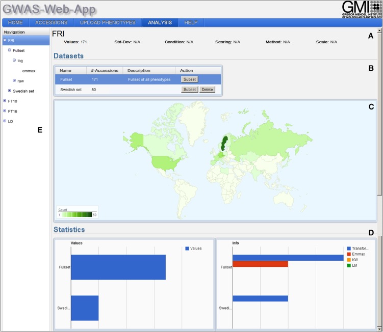
The phenotype view (Figure 1) is visible upon selecting a specific phenotype from the left navigation tree. Information is displayed in three related information panels. The top panel contains general information about the selected phenotype (Figure 1A). The center panel contains a list of all data sets, where a data set is defined as a subset of lines with phenotype values, together with the geographic distribution of the phenotyped accessions (Figures 1B and 1C). By default, every uploaded phenotype contains a “Fullset” data set that contains all the phenotype values available. The plot showing the geographical distribution is updated when a different data set (subset) is chosen. In the bottom panels (Figure 1D), basic statistics are shown for all the data sets.
Figure 1.
Phenotype View.
The phenotype view shows phenotype specific information in four panels. Panel (A) displays phenotype name and number of values. In (B), a list of data sets is shown. Selecting a data set from that list will update the geographic distribution map (C). Two bar charts in (D) show statistical information about the phenotype. The navigation tree on the left side (E) reflects the stored phenotype structure and is used to access different views.
Data Set View
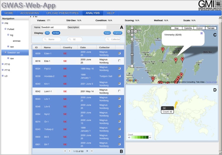
By choosing an existing data set or by creating a new one, the user is directed to the data set view (Figure 2). This view consists of a list of the accessions and two geographical plots. Using the list of accessions, the user can edit or create new data sets/subsets that contain, for example, only accessions from a specific country or collection. Using the list and the geographical map, the user can exclude, or include, certain accessions from specific regions. As different advantageous alleles can be expected to arise in some local adaptation scenarios (Chan et al., 2010), it may be beneficial for some traits to use regional data sets for mapping causal alleles.
Figure 2.
Data Set View.
(A) The filter box allows the user to exclude specific accessions as well as change the name and the description of the data set.
(B) The data set list displays information for each accession in the data set. In edit mode, the user can use the checkbox to add and remove accessions from the data set.
(C) A Google map shows the locations of all accessions in the data set. Clicking on one marker will show a pop-up with information about the name and ID of the selected accession.
(D) The geographic distribution map (GeoMap) shows the geographic distribution of the accessions in the data set. Moving the mouse over a country will show the number of accessions located in that region.
Transformation View
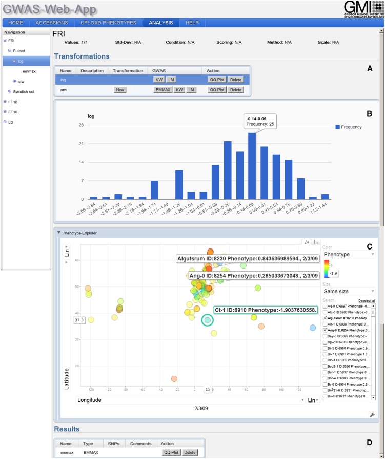
Applying a transformation to the phenotype may result in more reliable results for parametric tests. The transformation aims to facilitate the process of selecting a reasonable transformation, allowing the user to instantly preview the resulting phenotypic distribution. The view consists of four panels (Figure 3). The center panel (Figure 3C) contains a phenotype-explorer component (Huang et al., 2011), which, among other things, allows the user to plot phenotype values against latitude and longitude in a motion chart.
Figure 3.
Transformation View.
The transformation view consists of four panels. The list of stored transformations is displayed in (A). The use can create a new transformation, delete an existing one, or run one of three available GWAS analysis methods on the transformed phenotype values. Dependent on the selected transformation a histogram of the transformed phenotype values are displayed below the transformation list (B). The Accession-Phenotype-Explorer (C) visualizes additional accession information through a bar chart or a scatterplot. Panel (D) shows the stored GWAS results for the specific transformation.
The transformations implemented include logarithmic, square root, and Box-Cox transformations (Box and Cox, 1964). The P value for Shapiro-Wilks test for normality is reported in the histogram and may assist in choosing an appropriate transformation. However, we note that choosing an appropriate transformation in structured samples is not trivial since phenotypes are expected to have a multivariate distribution with non-zero correlations (Fisher, 1918). Since the phenotypes are not independent observations, their distribution may deviate from a bell-shaped univariate Gaussian distribution, even if they follow a multivariate Gaussian distribution. After deciding on a transformation, a genome-wide association scan can be performed. In the current version, the user can choose between (1) a nonparametric Wilcoxon rank sum test (Wilcoxon, 1945), (2) a simple linear regression (LM), and (3) an accelerated mixed model (AMM). AMM first performs a genome-wide scan using the approximate inference proposed by Zhang et al. (2010) and Kang et al. (2010) and then updates the smallest 100 P values using an exact mixed model inference (Kang et al., 2008). Both LM and AMM employ a parametric F-test to obtain the P values. For examining P value bias due to population stratification, one can use the Kolmogorov-Smirnov statistic, the median P value, as well as the QQ plots (Atwell et al., 2010).
Results View
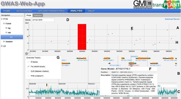
The results view has two main components that can be accessed via the Plots and Statistics tabs. Under the Plots tab, an interactive Manhattan plot (a scatterplot with the negative logarithm P values for the SNP association plotted against the SNP positions) for all five chromosomes is shown. The Benjamini-Hochberg-Yekutieli multiple testing procedure (Benjamini and Yekutieli, 2001) was used to control the false discovery rate. Assuming arbitrary dependence between SNPs, the 5% false discovery rate (FDR) threshold is plotted as a dashed horizontal line. Moving the mouse over a specific point in the plot will display the position of the corresponding SNP and its P value. The Manhattan plot supports zooming, which can be achieved by a “click, hold, and drag mouse” gesture that defines the area for the zoom action. If the zoom level is below a specific threshold (∼1.5 Mb), a gene annotation view (GeneViewer), which we developed specifically for this application, is displayed (Figure 4). Moving the mouse over a point in the Manhattan plot will also display a vertical line in the gene annotation view. If the zoom level is below 150 kb, a more detailed gene annotation view containing gene features (e.g., the coding sequence region and the untranslated regions will be shown). Moving the mouse over a specific gene in the GeneViewer will display a pop-up with additional functional description for the gene. Clicking on the gene will direct the user to The Arabidopsis Information Resource (TAIR) website for the gene, containing more detailed information. Finally, the user can highlight specific genes using a gene search field above the scatterplot for the first chromosome.
Figure 4.
Result View.
The result view displays GWAS plots for each of the five chromosomes. Each GWAS plot itself consists of three panels. The top panel (A) contains a scatterplot. The positions on the chromosome are on the x axis and the score on the y axis. The dots in the scatterplot represent SNPs (E). A horizontal dashed line (H) shows the 5% FDR threshold. At the top of the GWAS results view, a search box for genes is displayed (D). These genes will be displayed as a colored band (red in the figure). The second panel (B) shows the gene annotation and is only shown for a specific zoom range (<1.5 Mb). It will display genes, gene features, and gene names. Moving the mouse over a gene will display additional information in a pop-up (F), and clicking on a gene will open the TAIR page for the specific gene. Panel (C) displays various chromosome-wide statistics. The region highlighted by a yellow band (I) is shown in the scatterplot and in the gene annotation. The gear icon opens a pop-up (G) with the available statistics the user can choose from.
When the zoom level in the P value plot is below ∼1.5 Mb, a statistics panel is displayed below the gene annotations. By default, the statistics panel will show the gene density as a filled bar chart, but other statistics can be selected by clicking on the gears icon. Currently, five other statistics can be chosen: (1) Wright's fixation index, Fst, between north and south (Lewontin and Krakauer, 1973); (2) the composite likelihood ratio (CLR) from Sweepfinder (Nielsen et al., 2005); (3) the pairwise haplotype-sharing score (PHS) (Toomajian et al., 2006); (4) a recombination estimate (rho) (McVean et al., 2004); and (5) sequence similarity with Arabidopsis lyrata (Hu et al., 2011). Four of these statistics, Fst, CLR, PHS, and the recombination rate estimate, were calculated using the data set of Horton et al. (2012) and may not be representative for the subset being analyzed. In an attempt to address this issue, the user can upload statistics provided in a file with three comma-separated columns (chromosome, position, and value). This further enables the user to plot miscellaneous statistics underneath the Manhattan plots. All of the plotted statistics are binned and displayed in a similar interactive chart as the P values, which also allows for vertical and horizontal zooming. The region that the user has zoomed in on in the P value chart is highlighted in yellow. The bin size used to show the statistics can be adjusted by changing the number in the white text box in the lower left corner of the plot.
Users can also visualize the linkage disequilibrium (LD) structure. This can be done by clicking on any SNP and choosing from three different methods: (1) show LD in this region, (2) calculate exact LD in this region, and (3) highlight SNPs in LD for this SNP.
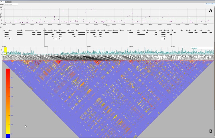
The first two options (“show LD in this region” and “calculate exact LD in this region”) display a LD triangle plot below the gene annotation panel and color code the SNPs in the Manhattan plot (Figure 5). The difference between the first two options is that the former only displays r2 values for the visible SNPs and the latter will calculate and show the r2 values of all SNPs regardless if they are displayed or not. Both options display pairwise r2 values of at most 500 SNPs (due to limitations regarding visualization and computational complexity). For the sake of visual clarity, only r2 values above 0.3 are color coded. Furthermore, selecting an SNP in the Manhattan plot will color code all neighboring SNPs according to their r2 value. At the same time, all pairwise r2 values in the triangle plot will be highlighted (see Supplemental Figure 2 online). Similarly, when a specific r2 value in the triangle plot is selected, the corresponding pair of SNPs in the Manhattan plot and the triangle plot is highlighted with corresponding color coding (see Supplemental Figure 3 online). Lastly, the third option (“highlight SNPs in LD for this SNP”) will calculate genome-wide r2 values between the selected SNP and all other displayed SNPs and color code them in the Manhattan plot (see Supplemental Figure 4 online).
Figure 5.
LD Visualization.
The LD is shown for a specific region with 500 SNPs. The triangle plot below (B) the gene annotation panel shows the r2 values for the 500 SNPs. Only r2 values above a certain threshold (0.3) are color coded, ranging from yellow (low) to red (high).
When using AMM, SNPs can be included as cofactors in the mixed model by clicking on a specific SNP and choosing “run conditional GWAS.” This allows the user to perform conditional analysis on both local and global scales. Including causal loci in the model has been shown to be beneficial for finding other causal markers in structured data (Segura et al., 2012; Vilhjálmsson and Nordborg, 2012). The second tab of the results view contains statistical descriptors and plots, which are useful when comparing models with different SNPs included as cofactors. These include three different model selection criteria: (1) the Bayesian information criterion (Schwarz, 1978), (2) the extended Bayesian information criterion (Chen and Chen, 2008), and (3) the multiple Bonferroni criterion (Segura et al., 2012). These model selection criteria can guide the user to select reasonable models (and cofactors) in the absence of other prior knowledge. AMM has the added advantage that it estimates the variance components, from which the overall narrow sense heritability estimates (also known as the pseudo-heritability) can be obtained. When cofactors are included and the analysis is rerun, these estimates are updated, providing an overview of how the phenotypic variance is partitioned among three categories: (1) the fixed effects (i.e., the variance explained by the SNP cofactors); (2) the random genetic term, which estimates the amount of unexplained variance attributable to genetics; and (3) the random error term, which is the fraction of variance attributed to random noise. These statistics provide a rough estimate of whether, and to what degree, further genetic effects can be detected. Hence, if the remaining genetic fraction of phenotypic variance is small, there may not be much reason for including more cofactors in the model.
A GWAPP Analysis Example for Flowering Time
To demonstrate how GWAPP can be used to make real biological discoveries, we use a flowering time data set published by Li et al. (2010). We focus on flowering time measured in 479 plants grown in growth chambers set to simulate Swedish spring conditions (Li et al., 2010). Flowering time in A. thaliana has been extensively studied with both linkage mapping (Salomé et al., 2011) and GWAS (Atwell et al., 2010; Brachi et al., 2010; Li et al., 2010). Furthermore, several genes have been shown to harbor genetic variants that affect flowering time, including FLOWERING LOCUS C (FLC) (Michaels and Amasino, 1999) and FRIGIDA (FRI) (Johanson et al., 2000).
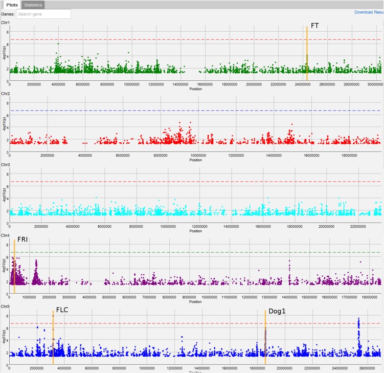
For the association mapping, we transformed the phenotypes using a logarithmic transformation, which yields values that generally cause extreme late flowering plants to be less extreme. We then used AMM to map the phenotype, resulting in several interesting regions (Figure 6), including ones harboring known flowering genes, such as FRI (Johanson et al., 2000), FLC, FLOWERING LOCUS T (FT) (Huang et al., 2005; Shindo et al., 2005), and DELAY OF GERMINATION1 (DOG1) (Alonso-Blanco et al., 2003; Bentsink et al., 2006) (although DOG1 is not a traditional candidate gene for flowering time, it has repeatedly been suggested to affect flowering time in recent GWAS studies; Atwell et al., 2010; Brachi et al., 2010; Li et al., 2010).
Figure 6.
First AMM Scan for Flowering Time.
A screenshot showing the first mixed-model scan for flowering time, highlighting the positions of four interesting candidate genes (FT, FRI, FLC, and DOG1) for which there seem to be associations.
Zooming in on the FRI gene (chromosome 4, position 269025 to 271503), we conditioned the most significant SNP within the gene [position 269260, −log(p) = 4.8]. This results in a very different association landscape around the FRI region, causing other SNPs near FRI to become significant at the 5% FDR threshold, where the SNP with the genome-wide smallest P value (negative log P value 7.7) was at position 264,496, <5 kb from the transcription start site of FRI (Figure 7). After adding this SNP to the model as a cofactor, both SNPs become significant at the 5% FDR threshold and appear to explain most of the signal in the region. These results are consistent with what is known about the role of FRI in flowering time (Aranzana et al., 2005; Shindo et al., 2005) (i.e., there are at least two segregating variants within and near FRI that affect flowering time). Given that the indels are in negative linkage disequilibrium, it is not surprising that the signal becomes more pronounced after conditioning on one SNP within FRI (Atwell et al., 2010; Platt et al., 2010). Although the two known causal variants are not included in the data set, because they are indels not SNPs, our analysis is still consistent with the known allelic heterogeneity.
Figure 7.
Conditional Mixed-Model Scans for Flowering Time.
The first AMM scan (A) without any cofactors is shown on the left. The second AMM scan (B) in the middle is the result from adding the SNP with the smallest P value within the FRI gene into the model as a cofactor. Finally, the third AMM scan (C) on the right is the result from adding the top SNP from the middle figure, which is 5 kb upstream of the FRI gene into the model as a cofactor. The negative log P values are shown on the y axis and the positions on the x axis. The 5% FDR threshold is denoted by a horizontal, dashed, green line.
We also included the most significant SNPs near known candidate genes, FLC, FT, and DOG1, in the model as cofactors. By doing so, many of the remaining peaks observed in the original scan dissipated (see Supplemental Figure 5 online), leading us to believe that they were synthetic associations (Dickson et al., 2010; Platt et al., 2010). However, two peaks on chromosome 5 still remain. The first of these is located in the pericentromeric region (12.51 to 12.56 Mb) and contains only a handful of genes, none of which are obvious candidates (see Supplemental Table 1 online). The second region (25.34 to 25.40 Mb) spans roughly 60 kb and includes SNPs with genome-wide significant P values. This region does not contain any obvious candidate genes (see Supplemental Table 2 online); however, it overlaps with a quantitative trait locus region recently observed for flowering time (Salomé et al., 2011).
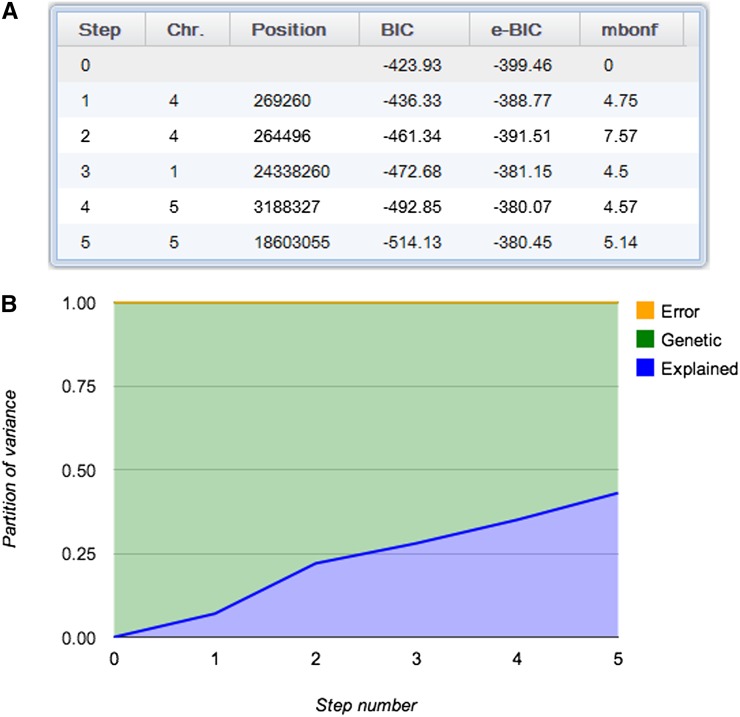
Finally, the mixed model estimated the narrow-sense heritability of flowering time to be 100%, which may seem extreme, but in fact is not far from the more robust broad-sense estimate of 92%. The five cofactors included in the model explained 43% of the phenotypic variance. The estimated fraction of remaining genetic variance was 57%, and the estimated fraction of remaining error variance was 0% (Figure 8). This indicates that there are still unexplained genetic effects in the genome, with the two remaining peaks on chromosome 5 as prime candidate regions.
Figure 8.
Partition of Variance for the Conditional Mixed-Model Scans.
Two screenshots showing the five SNPs included in the model (A) and how the partition of phenotypic variance changes as the five cofactors (FRI, FT, FLC, and DOG1) are added to the mixed model (B).
DISCUSSION
This article is part of our overall effort to enable the Arabidopsis community to capitalize on the unique resources of thousands of densely genotyped lines. Over 1300 lines have been genotyped using a 250k SNP chip (Horton et al., 2012), and a thousand more will be sequenced by the end of this year (Cao et al., 2011; Gan et al., 2011; www.1001genomes.org). It is our hope that these lines will be routinely phenotyped to reveal functionally important polymorphisms via GWAS. One obstacle to this becoming a reality is the difficulty of analyzing the data: Overcoming this difficulty is the direct objective of this work.
Our goal was to provide an easy-to-use tool for GWAS that enables users to focus on biology instead of spending time programming or converting file formats. All that is required is a simple import of the phenotypic data, which can easily be managed in a spreadsheet. GWAPP provides several interactive features, including the possibility of analyzing different subsets of the sample as well as some basic transformations of the raw phenotypic data. With interactive Manhattan and genome annotation plots, it is possible to browse through the results, zoom in on association peaks, and quickly gain an overview of what genes may harbor causal variants. Patterns of LD can analyzed, both local LD patterns as well as genome-wide LD patterns, which are calculated on-the-fly. To further aid interpretation, several statistics, including recombination rate and selection statistics, can be plotted along the chromosome. Conditional analysis using SNPs as cofactors makes it possible to investigate genetic heterogeneity, and estimates of variance components provide insight into the genetic architecture of the traits (Yang et al., 2010). Furthermore, GWAPP can do all this in minutes. Using similarly sized data sets for benchmarking, as used for the benchmarks in Matapax (Childs et al., 2012), we observed up to 50-fold increase in speed for a mixed model analysis of a single trait (see Methods).
To demonstrate how one might use GWAPP, we reanalyzed a previously published flowering time phenotype data set (Li et al., 2010). By leveraging a priori biological knowledge, we identified two independent loci near FRI, which when included in the mixed model explain a quarter of the total phenotypic variance. After including associated SNPs near four genes known to be involved in flowering time, there were still loci of potential interest. Interestingly, one of these is in a region that was recently shown to be associated with flowering time in a linkage mapping study (Salomé et al., 2011).
The Web application presented here, GWAPP, is a work in progress. It can be extended in several ways, and we are actively working on this. Most obviously, we will continuously increase the SNP data set by including overlapping SNP data from newly sequenced accessions (Cao et al., 2011; Gan et al., 2011). We will of course make it possible to use full sequence data from the 1001 genomes project, but this will require optimizations in order to run in real time. Another major improvement will be the ability to look for pleiotropy by looking for associations across all published phenotypic data. With the cooperation of the Arabidopsis community, it should be possible to establish a database that aims to functionally annotate every segregating polymorphism in the genome.
More trivially, the interface, tools, and methods can easily be changed, updated, and expanded based on user input. Finally, although GWAPP is currently dedicated to GWAS in A. thaliana, some parts of the application, including the interactive plots and the underlying data structures and mapping algorithms, can readily applied to data from other organisms, including humans. By structuring the application in modules, certain parts (e.g., interactive visualization components or the association mapping algorithms) can be easily reused for other projects. Importantly, all source code for our application is freely available.
METHODS
Genotype Data
The genotype data used was obtained by combining data from two different sources, namely, 1386 Arabidopsis thaliana accessions that were genotyped for 214k SNPs (Horton et al., 2012) and 80 A. thaliana accessions that were sequenced using next-generation sequencing (Cao et al., 2011). One accession (Fei-0) was characterized in both analyses (n = 1386), and we used the SNP calls from Horton et al., (2012) to correct the discordant SNP assignments (discordant rate was 2.5%). For the sequence data, we extracted the base calls corresponding to the 214k SNP positions from the combined matrix and imputed the missing alleles with BEAGLE version 3.3.1 (Browning and Browning, 2011). We used 30 iterations for the imputation, with the full merged data set as phased input. All triallelic SNPs were discarded for simplicity, leaving 206,087 SNPs in the final data set. The coordinates shown in the browser are TAIR 10 coordinates.
GWAPP does not provide any easy way to upload custom genotype data yet. However, users can download the virtual machine (VM) image of the application (see section VM image) and replace or extend the provided genotype data with custom ones.
Web Application
In order to minimize installation time and allow for widespread access, we implemented GWAPP as a Web application. The only client-side requirement is a browser that supports HTML5. The application consists of a back end, front end, and data exchange protocol (see Supplemental Figure 6 online). The server front end is the part of GWAPP that the user interacts with. The user interface and all visualization tools used for the analysis are a part of the front end. The front end is primarily implemented using modern Web technologies (HTML5 and Javascript). The back-end implements all association mapping methods, various statistics, and performs all handling of data, such as parsing, coordination, and filtering of phenotypes and genotypes. The back end is written almost entirely in Python and is all server side. Finally, the data exchange protocol communicates between the front end and the back end. The implementation details for the server (i.e., front end, back end, and the data exchange protocol) are described in Supplemental Methods 1 online.
VM Image
Since genotype data are typically large in size, GWAPP does not support uploading custom genotype data. Instead, we provide a shrink-wrapped package that has a version of GWAPP and all dependencies preinstalled and preconfigured as a VM image. The package also includes all nonstandard packages necessary for installation and deployment of GWAPP on either on-premise/private cloud or public cloud services. The VM image can be downloaded here: https://cynin.gmi.oeaw.ac.at/home/resources/gwapp/gwapp.
Further information for installing GWAPP locally is provided there, including information on how to use a different genotype data set than the Horton et al. (2012) data set: https://cynin.gmi.oeaw.ac.at/home/resources/gwapp/gwapp.
Mapping Methods
Three different mapping methods were implemented for GWAPP: a standard linear regression (LM), an AMM (Kang et al., 2010; Zhang et al., 2010), and a Wilcoxon rank sum test (Wilcoxon, 1945). AMM differs slightly from EMMAX (Kang et al., 2010) and P3D (Zhang et al., 2010), in that it reestimates the P values for the k = 100 most significant SNPs using exact inference (Kang et al., 2008; Lippert et al., 2011). The exact inference reestimates the variance components with the SNP in the model as a cofactor and then uses these updated variance components to reestimate the P value of that SNP. AMM has running time complexity of O(n2m+n3k), where n denotes the number of individuals and m the number of SNPs. If we choose k ≤ m/n, the running time becomes O(n2m) (i.e., the same as EMMAX [Kang et al., 2010], FaST-LMM [Lippert et al., 2011], and GEMMA [Zhou and Stephens, 2012]). Furthermore, LM and AMM were implemented to allow for inclusion of SNPs into the model (Segura et al., 2012) using the Gram-Schmidt process to ensure efficiency regardless of the number of cofactors included. See online methods in Segura et al. (2012) for further details. The three mapping methods were implemented in Python by extending mixmogam (https://github.com/bvilhjal/mixmogam) (Segura et al., 2012). We compiled SciPy (Jones et al., 2001) with the GotoBlas2 (Goto and Van de Geijn, 2008) Basic Linear Algebra Subroutines implementation on the publicly available GWAPP Web server. For AMM, the genetic relatedness matrix used is the identity by state (IBS) genetic relatedness matrix, which for a pair of individuals is the fraction of shared alleles among segregating SNPs in the sample. This is calculated a priori for the full genotype data set and then adjusted for each specific subset of accessions by removing the contributions of SNPs, which are not segregating the subset (monomorphic SNPs).
Runtime Analysis
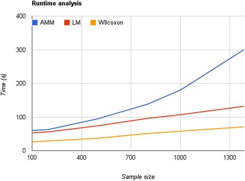
To benchmark the performance of GWAPP, six data sets were generated using random phenotype values (sampled from a uniform distribution), and using all 214k SNPs. The benchmark was conducted on the public Web server, where GotoBlas2 (which is used by AMM and LM for linear algebra operations) was configured to use up to four cores. The time was measured from pressing the analysis method button until all the P values were displayed in the Manhattan plots. All three mapping methods finished within 5 min for all the data sets (Figure 9). AMM was considerably slower than the other two, but all methods finished the analysis within 2 min when using <500 individuals. This is ∼50 times faster than Matapax (Childs et al., 2012), which required more than 1 h to run on 500 individuals using a single trait and a similar sized genotype data set.
Figure 9.
Runtime for Different Mapping Methods.
The time, from starting the analysis until the P values are visible in the Manhattan plot, is plotted against the number of individuals used for the GWAS. Lines for all three mapping methods are shown: AMM, LM, and the Wilcoxon rank sum test.
Accession Numbers
The four candidate genes for flowering time have the following Arabidopsis Genome Initiative locus identifiers: FRI (At4g00650), FLC (At5g10140), FT (At1g65480), and DOG1 (At5g45830). The genotype data can be found here: https://cynin.gmi.oeaw.ac.at/home/resources/atpolydb/250k-snp-data/call_method_82.tar.gz/view. GWAPP can be accessed at: http://gwas.gmi.oeaw.ac.at. All code is public and can be obtained at https://github.com/timeu/GWAPP.
Supplemental Data
The following materials are available in the online version of this article.
Supplemental Figure 1. Analysis Levels of GWAPP.
Supplemental Figure 2. LD Visualization: Highlighting an SNP.
Supplemental Figure 3. LD Visualization: Highlighting an r2 Value.
Supplemental Figure 4. Genome-Wide LD Visualization.
Supplemental Figure 5. AMM Scan after Conditioning on Five SNPs.
Supplemental Figure 6. Overview of the Web Application Structure.
Supplemental Table 1. Genes Located in a Region (12.51 to 12.56 Mb) on Chromosome 5, Which Displayed Association with Flowering Time.
Supplemental Table 2. Genes Located in a 60-kb Region (25.34 to 25.39 Mb) on Chromosome 5, Which Displayed Association with Flowering Time.
Supplemental Methods 1. GWAPP Implementation Details.
Acknowledgments
We thank Arthur Korte, Envel Kerdaffrec, Fernando Rabanal, Wolfgang Busch, Danielle Filiault, and others for testing the software and providing feedback. We also thank Geoff Clarck for his useful comments. This work was supported by grants from the European Union Framework Programme 7 (TransPLANT, grant agreement 283496) to M.N. as well as by the Austrian Academy of Sciences through the Gregor Mendel Institute.
AUTHOR CONTRIBUTIONS
Ü.S., B.J.V., V.S., and M.N. designed the study. Ü.S. and B.J.V. implemented and coded the Web application with help from Y.S.H. M.W.H. and Q.L. provided genome-wide statistics. D.M. and B.J.V. prepared the genotype data. P.F. and Ü.S. set up the server. Ü.S., B.J.V., and M.N. wrote the article with input from all authors.
Glossary
- GWAS
genome-wide association studies
- SNP
single nucleotide polymorphism
- LM
linear regression
- AMM
accelerated mixed model
- TAIR
The Arabidopsis Information Resource
- LD
linkage disequilibrium
- VM
virtual machine
References
- Alonso-Blanco C., Bentsink L., Hanhart C.J., Blankestijn-de Vries H., Koornneef M. (2003). Analysis of natural allelic variation at seed dormancy loci of Arabidopsis thaliana. Genetics 164: 711–729 [DOI] [PMC free article] [PubMed] [Google Scholar]
- Aranzana M.J., et al. (2005). Genome-wide association mapping in Arabidopsis identifies previously known flowering time and pathogen resistance genes. PLoS Genet. 1: e60. [DOI] [PMC free article] [PubMed] [Google Scholar]
- Atwell S., et al. (2010). Genome-wide association study of 107 phenotypes in Arabidopsis thaliana inbred lines. Nature 465: 627–631 [DOI] [PMC free article] [PubMed] [Google Scholar]
- Baxter I., Brazelton J.N., Yu D., Huang Y.S., Lahner B., Yakubova E., Li Y., Bergelson J., Borevitz J.O., Nordborg M., Vitek O., Salt D.E. (2010). A coastal cline in sodium accumulation in Arabidopsis thaliana is driven by natural variation of the sodium transporter AtHKT1;1. PLoS Genet. 6: e1001193. [DOI] [PMC free article] [PubMed] [Google Scholar]
- Benjamini Y., Yekutieli D. (2001). The control of the false discovery rate in multiple testing under dependency. Ann. Stat. 29: 1165–1188 [Google Scholar]
- Bentsink L., Jowett J., Hanhart C.J., Koornneef M. (2006). Cloning of DOG1, a quantitative trait locus controlling seed dormancy in Arabidopsis. Proc. Natl. Acad. Sci. USA 103: 17042–17047 [DOI] [PMC free article] [PubMed] [Google Scholar]
- Box G.E.P., Cox D.R. (1964). An analysis of transformations. J. R. Stat. Soc. B 26: 211–252 [Google Scholar]
- Brachi B., Faure N., Horton M.W., Flahauw E., Vazquez A., Nordborg M., Bergelson J., Cuguen J., Roux F. (2010). Linkage and association mapping of Arabidopsis thaliana flowering time in nature. PLoS Genet. 6: e1000940. [DOI] [PMC free article] [PubMed] [Google Scholar]
- Bradbury P.J., Zhang Z., Kroon D.E., Casstevens T.M., Ramdoss Y., Buckler E.S. (2007). TASSEL: Software for association mapping of complex traits in diverse samples. Bioinformatics 23: 2633–2635 [DOI] [PubMed] [Google Scholar]
- Browning B.L., Browning S.R. (2011). A fast, powerful method for detecting identity by descent. Am. J. Hum. Genet. 88: 173–182 [DOI] [PMC free article] [PubMed] [Google Scholar]
- Cao J., et al. (2011). Whole-genome sequencing of multiple Arabidopsis thaliana populations. Nat. Genet. 43: 956–963 [DOI] [PubMed] [Google Scholar]
- Chan Y.F., et al. (2010). Adaptive evolution of pelvic reduction in sticklebacks by recurrent deletion of a Pitx1 enhancer. Science 327: 302–305 [DOI] [PMC free article] [PubMed] [Google Scholar]
- Chen J.H., Chen Z.H. (2008). Extended Bayesian information criteria for model selection with large model spaces. Biometrika 95: 759–771 [Google Scholar]
- Childs L.H., Lisec J., Walther D. (2012). Matapax: An online high-throughput genome-wide association study pipeline. Plant Physiol. 158: 1534–1541 [DOI] [PMC free article] [PubMed] [Google Scholar]
- Dickson S.P., Wang K., Krantz I., Hakonarson H., Goldstein D.B. (2010). Rare variants create synthetic genome-wide associations. PLoS Biol. 8: e1000294. [DOI] [PMC free article] [PubMed] [Google Scholar]
- Fisher R.A. (1918). The correlation between relatives on the supposition of Mendelian inheritance. Trans. R. Soc. Edinb. 52: 399–433 [Google Scholar]
- Gan X., et al. (2011). Multiple reference genomes and transcriptomes for Arabidopsis thaliana. Nature 477: 419–423 [DOI] [PMC free article] [PubMed] [Google Scholar]
- Goto K, Van de Geijn R. (2008). High-performance implementation of the level-3 BLAS. ACM Trans. Math. Softw. 35: 4:1–4:14. [Google Scholar]
- Horton M.W., et al. (2012). Genome-wide patterns of genetic variation in worldwide Arabidopsis thaliana accessions from the RegMap panel. Nat. Genet. 44: 212–216 [DOI] [PMC free article] [PubMed] [Google Scholar]
- Hu T.T., et al. (2011). The Arabidopsis lyrata genome sequence and the basis of rapid genome size change. Nat. Genet. 43: 476–481 [DOI] [PMC free article] [PubMed] [Google Scholar]
- Huang Y.S., Horton M.W., Vilhjálmsson B.J., Seren Ü., Meng D., Meyer C., Ali Amer M., Borevitz J.O., Bergelson J., Nordborg M. (2011). Analysis and visualization of Arabidopsis thaliana GWAS using Web 2.0 technologies. Database (Oxford) 2011: bar014. [DOI] [PMC free article] [PubMed] [Google Scholar]
- Johanson U., West J., Lister C., Michaels S., Amasino R., Dean C. (2000). Molecular analysis of FRIGIDA, a major determinant of natural variation in Arabidopsis flowering time. Science 290: 344–347 [DOI] [PubMed] [Google Scholar]
- Jones E., et al. (2001). SciPy: Open source scientific tools for python. http://www.scipy.org
- Kang H.M., Sul J.H., Service S.K., Zaitlen N.A., Kong S.Y., Freimer N.B., Sabatti C., Eskin E. (2010). Variance component model to account for sample structure in genome-wide association studies. Nat. Genet. 42: 348–354 [DOI] [PMC free article] [PubMed] [Google Scholar]
- Kang H.M., Zaitlen N.A., Wade C.M., Kirby A., Heckerman D., Daly M.J., Eskin E. (2008). Efficient control of population structure in model organism association mapping. Genetics 178: 1709–1723 [DOI] [PMC free article] [PubMed] [Google Scholar]
- Lewontin R.C., Krakauer J. (1973). Distribution of gene frequency as a test of the theory of the selective neutrality of polymorphisms. Genetics 74: 175–195 [DOI] [PMC free article] [PubMed] [Google Scholar]
- Li Y., Huang Y.S., Bergelson J., Nordborg M., Borevitz J.O. (2010). Association mapping of local climate-sensitive quantitative trait loci in Arabidopsis thaliana. Proc. Natl. Acad. Sci. USA 107: 21199–21204 [DOI] [PMC free article] [PubMed] [Google Scholar]
- Lipka A.E., Tian F., Wang Q., Peiffer J., Li M., Bradbury P.J., Gore M.A., Buckler E.S., Zhang Z. (2012). GAPIT: Genome association and prediction integrated tool. Bioinformatics 28: 2397–2399 [DOI] [PubMed] [Google Scholar]
- Lippert C., Listgarten J., Liu Y., Kadie C.M., Davidson R.I., Heckerman D. (2011). FaST linear mixed models for genome-wide association studies. Nat. Methods 8: 833–835 [DOI] [PubMed] [Google Scholar]
- McVean G.A., Myers S.R., Hunt S., Deloukas P., Bentley D.R., Donnelly P. (2004). The fine-scale structure of recombination rate variation in the human genome. Science 304: 581–584 [DOI] [PubMed] [Google Scholar]
- Michaels S.D., Amasino R.M. (1999). FLOWERING LOCUS C encodes a novel MADS domain protein that acts as a repressor of flowering. Plant Cell 11: 949–956 [DOI] [PMC free article] [PubMed] [Google Scholar]
- Nielsen R., Williamson S., Kim Y., Hubisz M.J., Clark A.G., Bustamante C. (2005). Genomic scans for selective sweeps using SNP data. Genome Res. 15: 1566–1575 [DOI] [PMC free article] [PubMed] [Google Scholar]
- Platt A., Vilhjálmsson B.J., Nordborg M. (2010). Conditions under which genome-wide association studies will be positively misleading. Genetics 186: 1045–1052 [DOI] [PMC free article] [PubMed] [Google Scholar]
- Salomé P.A., Bomblies K., Laitinen R.A.E., Yant L., Mott R., Weigel D. (2011). Genetic architecture of flowering-time variation in Arabidopsis thaliana. Genetics 188: 421–433 [DOI] [PMC free article] [PubMed] [Google Scholar]
- Schwartz C., et al. (2009). Cis-regulatory changes at FLOWERING LOCUS T mediate natural variation in flowering responses of Arabidopsis thaliana. Genetics 183: 723–732 [DOI] [PMC free article] [PubMed] [Google Scholar]
- Schwarz G.E. (1978). Estimating the dimension of a model. Ann. Stat. 6: 461–464 [Google Scholar]
- Segura V., Vilhjálmsson B.J., Platt A., Korte A., Seren Ü., Long Q., Nordborg M. (2012). An efficient multi-locus mixed-model approach for genome-wide studies in structured populations. Nat. Genet. 44: 825–830 [DOI] [PMC free article] [PubMed] [Google Scholar]
- Shindo C., Aranzana M.J., Lister C., Baxter C., Nicholls C., Nordborg M., Dean C. (2005). Role of FRIGIDA and FLOWERING LOCUS C in determining variation in flowering time of Arabidopsis. Plant Physiol. 138: 1163–1173 [DOI] [PMC free article] [PubMed] [Google Scholar]
- Svishcheva G.R., Axenovich T.I., Belonogova N.M., van Duijn C.M., Aulchenko Y.S. (2012). Rapid variance components-based method for whole-genome association analysis. Nat. Genet. 44: 1166–1170 [DOI] [PubMed] [Google Scholar]
- Todesco M., et al. (2010). Natural allelic variation underlying a major fitness trade-off in Arabidopsis thaliana. Nature 465: 632–636 [DOI] [PMC free article] [PubMed] [Google Scholar]
- Toomajian C., Hu T.T., Aranzana M.J., Lister C., Tang C., Zheng H., Zhao K., Calabrese P., Dean C., Nordborg M. (2006). A nonparametric test reveals selection for rapid flowering in the Arabidopsis genome. PLoS Biol. 4: e137. [DOI] [PMC free article] [PubMed] [Google Scholar]
- Vilhjálmsson B.J., Nordborg M. (2012). The nature of confounding in genome-wide association studies. Nat. Rev. Genet. 14: 1–2. [DOI] [PubMed] [Google Scholar]
- Wilcoxon F. (1945). Individual comparisons by ranking methods. Biom. Bull. 1: 80–83 [Google Scholar]
- Yang J.A., Benyamin B., McEvoy B.P., Gordon S., Henders A.K., Nyholt D.R., Madden P.A., Heath A.C., Martin N.G., Montgomery G.W., Goddard M.E., Visscher P.M. (2010). Common SNPs explain a large proportion of the heritability for human height. Nat. Genet. 42: 565–569 [DOI] [PMC free article] [PubMed] [Google Scholar]
- Yu J.M., Pressoir G., Briggs W.H., Vroh Bi I., Yamasaki M., Doebley J.F., McMullen M.D., Gaut B.S., Nielsen D.M., Holland J.B., Kresovich S., Buckler E.S. (2006). A unified mixed-model method for association mapping that accounts for multiple levels of relatedness. Nat. Genet. 38: 203–208 [DOI] [PubMed] [Google Scholar]
- Zhao K.Y., Aranzana M.J., Kim S., Lister C., Shindo C., Tang C., Toomajian C., Zheng H., Dean C., Marjoram P., Nordborg M. (2007). An Arabidopsis example of association mapping in structured samples. PLoS Genet. 3: e4. [DOI] [PMC free article] [PubMed] [Google Scholar]
- Zhang Z.W., Ersoz E., Lai C.-Q., Todhunter R.J., Tiwari H.K., Gore M.A., Bradbury P.J., Yu J., Arnett D.K., Ordovas J.M., Buckler E.S. (2010). Mixed linear model approach adapted for genome-wide association studies. Nat. Genet. 42: 355–360 [DOI] [PMC free article] [PubMed] [Google Scholar]
- Zhou X., Stephens M. (2012). Genome-wide efficient mixed-model analysis for association studies. Nat. Genet. 44: 821–824 [DOI] [PMC free article] [PubMed] [Google Scholar]


